Redshift Estimation Using Interpretable Machine Learning 

Abstract

The ΛCDM model, which, in its most basic formulation, consists of six cosmological parameters, can predict a number of independent cosmological phenomena. The Hubble Constant, one of the parameters of the model, highly depends on the redshift. Calculating redshift involves either estimation from photometric data (photo-z’s) or finding the true redshift from spectral emission line data (spec-z’s). Pipelines such as ANNz, which are neural-network-based, are more complex models, reach the lowest error but produce noisier, less-interpretable results. This manuscript matches precision of state-of-the-art ANN models with traditional ML techniques, using precise feature engineering, to produce more interpretable results. We revolve the discussion around our models’ interpretability via the accuracy and comparability of our results (as they will be used for mapping the universe and for cosmological modeling) along with the astrophysical mechanisms to analyze feature importances. The data, created by cross-matching the WISE catalog with the superCOSMOS redshift values, consists of a total of six magnitudes and galaxies in the low-redshift region (z<1). Our best performance was exhibited using light gradient boosting, and the overall RMSE was 0.0362. These results offer an alternative method to estimate the redshift in light of future cosmological experiments.

Introduction

Basic Cosmological Theory and connections to the research 

The prevailing cosmological model, ΛCDM, makes a series of accurate, independent predictions of cosmological phenomena¹. Its basic formulation consists of six independent (cosmological) parameters, which cannot be derived from theory. One such cosmological parameter is Hubble’s constant, which has an average, theoretically calculated, value of 68 km/s/Mpc at z=0 and t=present day. This parameter measures the rate at which the universe expands and is determined by calculating H(0) from the ΛCDM model. This constant is highly dependent on the galaxies’ redshift, and it is used in Hubble’s law to calculate the recessional velocities of galaxies. Hubble’s law is defined as: 

(1)  

where v is the recessional velocity, d is the distance from Earth, and is Hubble’s Constant. The cosmological redshift z is defined as:

(2)  

Where the is the observed wavelength of the galaxy, and the is the standard wavelength of the band^1,2,3. 

Since major astronomical surveys have been cataloging the universe, the cosmological redshift has been found primarily from the galaxy spectral emission line data (hereafter known as the spectroscopic redshift (spec-z)), which is time-consuming. So spec-z is now typically estimated from the photometric data (e.g., galaxies’ magnitudes, fluxes, colors, spectral energy distributions (SEDs which are graphs of the flux against wavelength for a galaxy), etc)³, which is known as photometric redshift (photo-z)³. Also, with the advancement of machine learning and computational methods, astronomers have started producing photo-z values by either fitting templates or training neural networks on photometric data, and it has been realized in the last decade that machine learning is the way to produce accurate photo-z values efficiently⁴. Moreover, using machine learning models to estimate redshift benefits cosmological modeling, mapping the universe (especially the distribution of galaxies and dark matter), and aiding future and current surveys, such as the LSST⁵; Euclid surveys⁶; SDSS-V⁷, by efficiently producing accurate photo-z’s. However, it has been shown that neural networks have reached their limits at producing accurate photo-z values and that traditional machine learning methods could pick up where they left off, as shown in the study conducted by Norris et al.^8,3,4,9,6,7.

Fitting templates versus training machine learning to find the photo-z 

In 1962, Baum proposed the first technique for estimating redshift⁸, and branching out from his work, many studies have commonly used either template-fitting or training neural networks to calculate photo-z. Templates are collections of SEDs. Training various neural networks, such as the artificial (networks where the information is fed forward through the layers with no memory of the previous inputs) and recurrent (networks where the data is looped and remembered) networks, on photometric data, has, insofar, produced the lowest root-mean squared error (RMSE) between the predictions and the true redshift (spec-z)¹⁰. Most of the photometric data comes from astronomical surveys, such as the abovementioned ones. The two methods share a common goal of finding the optimal z-function that inputs photometric or spectroscopic data and maps it into a singular photo-z value^4,8,11,10. 

The templates can either be generated through observation or computational models (e.g., Stellar Population Synthesis models), which output the average SEDs of the galaxies in space. Bruzual and Charlot’s study (1993) was the first to use this by using templates that are representative of the testing set and best minimize the χ² error, defined as 

(3)  

(4)  

where f_i is flux in the i-th band for a testing point, σ²_i is the square of the error of the flux in the ith filter, t_i(z, SED) is the flux in the ith filter for a given SED and z, and ɑ(z, SED) is the normalized template with respect to the observed template flux. The redshift of the template that has the lowest error with the testing galaxy in question will be assigned to that galaxy. The most common library of templates used is the one from Coleman, Wu, and Weedman’s study (CWW 1980). Equation 3 relates the error to the aforementioned variables, which the template fitting methods rely on; furthermore, equation 4 relates the normalized template metric, which is one of the metrics that the template fitting methods rely on, to the same metrics as mentioned above. Practically, the error is a traditional error metric used for certain machine learning fitting methods, similar to the common regression metrics such as RMSE and mean absolute error (MAE), which in training should be minimized^4,8,11,10.

The template methods’ ease of implementation is an advantage, but their accuracy depends on the ability of the templates to represent the testing set’s data distribution. These methods tend to perform better in cases with considerable prior knowledge about the data^4,8,11,10. The methods aforementioned, which produce the templates, often cannot produce ones that match the testing set’s distribution and are impractical as they take time and resources to create. Furthermore, SEDs are made by measuring just the luminous center of galaxies, as that is the light that hits the spectrograph, unlike tabular photometric data, which takes all of the light from the galaxy⁴. In contrast to the template-fitting methods, training neural networks on photometric data produces a lower RMSE error, can be trained over a larger dataset (as long as the training and testing data’s distributions are the same), and can predict up to z=1 (there is a certain limit after which machine learning models cannot predict the redshift for)^4,8,11,10.

From a comprehensive review of the literature^4,8,11,10, we have seen that the computationally complex neural networks (specifically the ANNz model) have obtained the lowest RMSE. However, now more commonly, the traditional machine models are being used and have been found to produce a lower RMSE compared to neural networks, but they have been trained on limited and small datasets⁷. We hypothesize that we can match the state-of-the-art ANNz model with traditional machine learning techniques trained on similar data-rich and big sets used to train the neural networks, using precise feature engineering, to produce better, more interpretable results. We measure the interpretability of our models by the accuracy of our results (as they will be used for mapping the universe and for cosmological modeling) and the models’ algorithmic and computational simplicity^4,8,11,10. To obtain our data, we cross-matched the WISE catalog with the corresponding spec-z and photo-z values from the superCOSMOS catalog. Of all of our models, the Light-gradient boosting machine (LGBM) regressor obtained the lowest RMSE of 0.0362, which is 2% lower than the RMSE of the state-of-the-art ANNz model, and all of our models’ RMSE fell within a range of 0.0362–0.0379. From the feature importances, we observed that the colors containing the magnitudes at the ends of the infrared and visible ranges had the most importance with the models^4,8,11,10.

Methodology

Data Collection and Pre-Processing: 

Our data came from the WISE¹² and SuperCOSMOS¹³ survey catalogs. The redshifts in the SuperCOSMOS survey were obtained by training the ANNz model on the GAMA-II data, as done by Bilicki et al¹⁴. In the study, Bilicki et. al¹⁴ obtained a deep, wide-angle galaxy sample that is approximately 95% pure (this means that the sample is 95% correctly labeled with 5% of the objects are misclassified) and 90% complete (this means that 90% of the total number of galaxies in the sky within the survey’s observation limits are recorded) at high Galactic latitudes, which was done after cleaning the data of inherent noise and images that could be confused as galaxies, which were stars. Their catalog contains nearly 20 million galaxies over almost 70% of the sky, and the data is outside regions in which galaxies could be confused with other astronomical objects, with a mean surface density of more than 650 sources per square degree^12,13,14.

We cross-matched the WISE catalog with the corresponding spec-z and photo-z from the SuperCOSMOS catalog to create our primary dataset, and we removed the galaxies that did not have a defined spec-z value (the SuperCOSMOS catalog did not have spec-z values for all of the data points due to the inherent limitations of spectroscopic samples) and that were on the galactic plane. We removed the galactic plane galaxies using the HealPy library¹⁵, which Astronomers use to deal with large amounts of galactic data¹⁵, because those galaxies’ magnitudes would be redshifted due to the intergalactic gas on that plane absorbing the light from those galaxies. The final dataset, after these two aforementioned processes were performed, was then put into feature-engineering pipelines to prepare it for training the models. Finally, our dataset had a total of 1341577 galaxies (Figure 1)¹⁵.

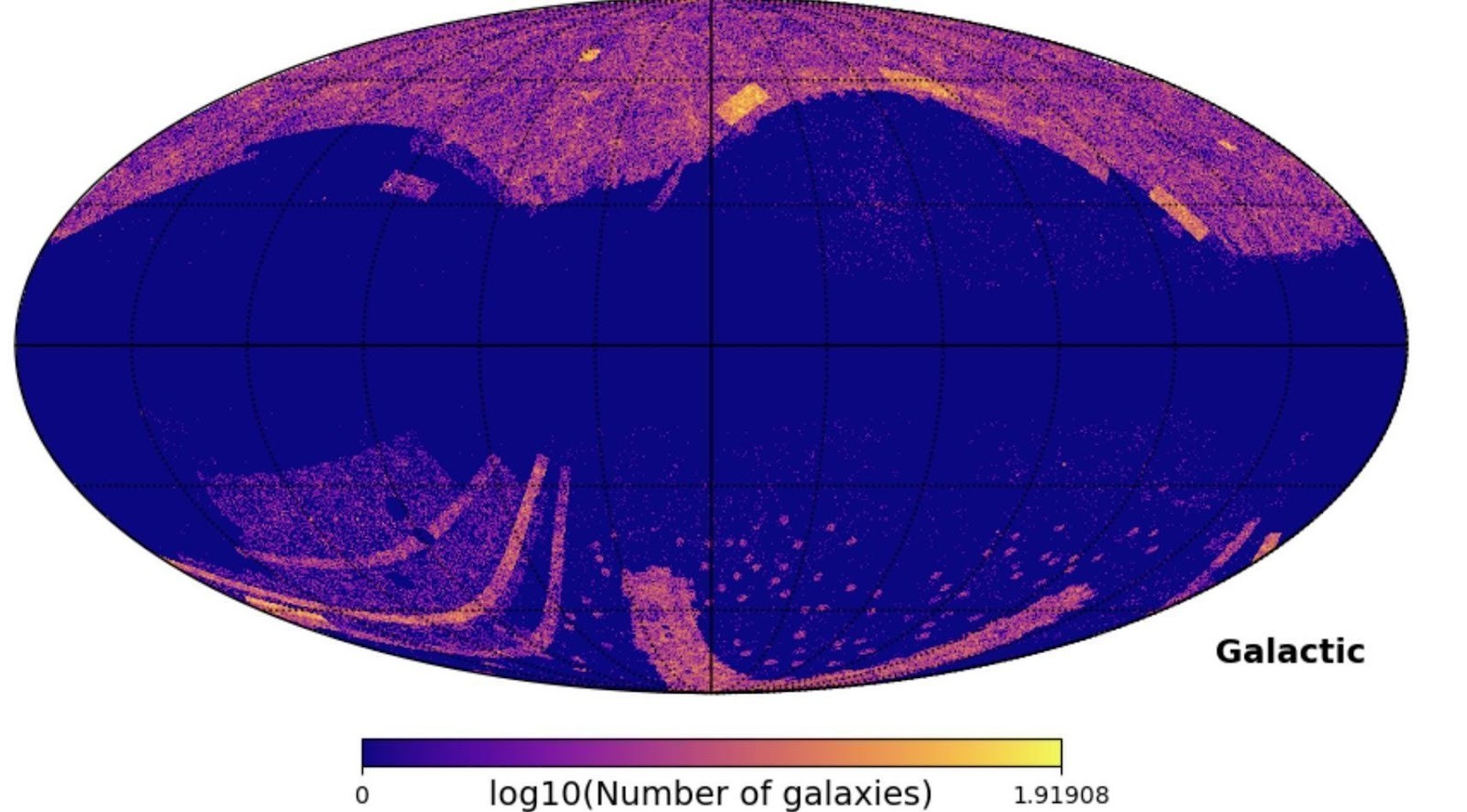
Figure 1 | The galactic map. A  map of the galaxies in our dataset minus the galactic mask (A list of the galaxies that lie in our galactic plane, where the blue space represents those galaxies). Using the Healpy library¹⁵, we first converted the galactic coordinates of each galaxy to the spherical coordinate system, and then we plotted the galaxies with a certain resolution defined by the pixel count. We use galactic coordinates to showcase the galaxy in the middle of the Figure. 

Next, we added features (dataset columns) to our dataset so that there could be many features for the models to train on and to make them more robust. The original data came with six magnitudes from the visible light spectrum and two magnitudes from the infrared spectrum (Table 3). We removed the coordinate columns and added twenty-eight color columns and one color excess column. We defined color excess

(5)  

where W₁ and W₂ are infrared spectrum magnitudes at the ends, and R and B are visible spectrum magnitudes at the ends (Table 1). 

Name of Magnitude	Wavelength range	Central Wavelength
B	400-500 nm	~450 nm
R	550-800 nm	~675 nm
I	700-900 nm	~800 nm
J	1.235 m	1.235 m
H	1.662 m	1.662 m
K	2.159 m	2.159 m
W1	3.4 m	3.4 m
W2	4.6 m	4.6 m

Next, we ran the data through the Principal Component Analysis (PCA) algorithm, and we then determined which principal components had a sum of explained variance (a measure of how much of the variance is explained by a set of independent variables) greater than 99.5% (removing the data that had a sum of explained variance less than 99.5% did not impact the overall results of the model because it removed little information). We then created a separate dataset from the eigenvalues of these components (hereafter known as the PCA dataset).

Brief description of the EDA algorithms 

We used the exploratory data analysis (EDA) algorithms, where we plotted the data in gaussian-kde histograms, a PCA plot, and a UMAP plot (Figures 2 and 3) using the scikit-learn and umap-learn libraries^16,17. The Gaussian KDE plots are 2D histograms that use the Gaussian kernel to bin the data (Figure 3) to visualize the correlation between the many features of the data. We implemented the Uniform Manifold Approximation and Projection (UMAP) algorithms. Both PCA and UMAP utilize their standard implementations. The UMAP algorithm projects the data into the Cartesian plane by finding the nearest neighbors to each point, weighting each neighbor based on distance, and then squishing the data into clusters in two dimensions (Figure 2)^16,17. 

The UMAP plot clearly shows the boundaries between the different regions of redshift ranges; for example, the red data cluster marks a well-defined region of redshift, which does not bleed into the other regions as much as it did in the PCA plot. This is probably due to the algorithm, which plots each data point based on its nearest neighbors (Figure 2). From the UMAP plot, we can see the clear redshift regions defined within our data. Although our data is considered within the low-redshift region, there are still sub-regions within the data. This can show that there could be a very clear distinction in the data for each region. For example, the purple region probably has different ranges of each feature than the red region (Figure 2)^16,17.

 

An overview of the Machine-learning algorithms 

We utilize seven traditional Machine Learning models using Python’s scikit-learn and tensorflow libraries^17,20: k-nearest neighbors (kNN), Random Forest, support-vector machine (SVM), Adaptive-boosting Forest, Histogram-Gradient-boosting Forest, Light-Gradient-boosting Forest, and Feed-Forward Neural Network algorithms (a type of Artificial Neural Network). The kNN, SVM, and Random Forest utilize their standard scikit-learn implementation, while the other three algorithms are different variations of the Random Forest algorithm (e.g., some use the boosting method instead of the bagging method)^17,20. 

1. The k-nearest neighbors (kNN) algorithm: Our kNN model, which utilizes the standard scikit-learn algorithm, uses the ball-tree optimization algorithm. The ball-tree algorithm separates a multidimensional space into k spherical sections and finds the distances between the testing point and the boundary of the section and between the testing point and its neighbor. It then creates a decision tree and separates the data based on whether the distance between the testing point and the neighbor is greater or less than the distance between the testing point and the boundary of the section. The decision tree then determines that if the distance of the neighbor to the test point is greater than the distance between the test point and the boundary, then it’s not a nearest neighbor. The ball-tree algorithm splits only the area of the feature space in which the points exist, making it more optimal to use in higher-dimensional feature spaces (d ≥ 3). Our data set includes 37 dimensions, so we choose to implement the ball-tree algorithm to reduce the computation time used by the kNN algorithm^4,21.  
2. Adaptive Boosting Forest Regressor: The AdaBoost model was created with the scikit-learn library. The AdaBoost calculates the weighted error rate of the predictions of the individual Decision Trees (it takes the points with more weight into account) and the weight of the tree itself. Then it updates the weights of each data point, where the data points that are wrong get assigned higher weights and affect the total weight of the tree. These steps repeat until all trees have a prediction; the final output matrix is a sum of the product between the predicted value and the weight of the tree that produced that prediction ^17,22,23.
3. Gradient-Boosting Forest Regressors: The Histogram-Gradient-Boosting model was created with the scikit-learn library, and the Light Gradient Boosting Machine (LGBM) model was created with the Light-GBM library. The gradient boosting models work by calculating the error rate of each tree. Then it updates the inputs of the next tree with the error calculated in the previous step. These two steps repeat until it reaches the final tree. The final prediction is the sum of the predictions of all of the individual trees. The LGBM and Hist-GBM models work by following the aforementioned algorithm, but they additionally implement histogram-based training, which is when the data is binned (a bin is a 2D histogram containing certain statistics, such as the gradient or a feature, against the frequency). Additionally, LGBM implements a leaf-growth algorithm where it selects the nodes that reduce the loss function the most and puts them in the trees ^17,22,23.

Training the machine learning models: 

We trained the machine-learning algorithms by implementing the sci-kit-learn’s experimental Halving-Random-Search-Cross-Validation class. We chose this one instead of the Grid-search-cross-validation class because it is computationally efficient, uses resources better, prevents overfitting on the validation sets, searches parameter space more efficiently, and finds the optimal parameter values with a minimized error^17,24,25. Since there were a lot of missing entries in this dataset, we had to use an iterative imputing method to fill them in. We also used the robust scaling method, which transforms the data by aligning the percentiles to those of the normal distribution. Then, we created two datasets from the original data, one of which did not contain the outliers of the data. Similarly, we created two datasets from the Principal Component Analysis (PCA) dataset, one of which did not contain the outliers of the data. Then, using these four datasets, we ran four iterations of the Halving-Random search to train the models^17,24,25. 

In the process of training the models, we used the Halving-random search method along with the robust scaler and iterative imputing methods to prepare the data for the model training. In the Halving-random search, we a trained an SVM regression model with testable kernels of linear or rbf and testable C values of 10^-2 to 10³ in steps of 10, and we trained a kNN regression model with a set ball tree search algorithm and testable k values of 5 to 500 in steps of 50. Moreover, we trained 4 types of forest-based algorithms with one extension of the standard random forest model: the extra trees regressor. We trained the random forest and extra regressors with a testable number of trees from 100 to 1000 in steps of 50, a testable max depth range from 3 to 9 in steps of 1,  a testable range of the minimum number of samples required per leaf from 200 to 5 in steps of 5, and lastly, a testable range of the max number of features from 0.6 to 0.8 in steps of 1. Next, we trained the LGBMRegressor with testable ranges of the number of trees from 100 to 1000 in steps of 50, of the max depth from 3 to 9 in steps of 1, of the learning_rate to be either 0.01 0.1, 0.3, or 1.0, of the number of leaves from 30 to 50 in steps of 100, of the minimum number of datapoints in a leaf from 200 to 20 in steps of 20, and of the fraction of features used from 0.6 to 0.8, in steps of 1.0. Then, we trained the Histogram-Gradient-Boosting Regressor with testable ranges of the maximum iterations from 100 to 1000 in steps of  50, of the max depth from 3 to 9 in steps 1, of the learning rate as either 0.01, 0.1, 0.3, or 1.0, and of the max fraction of features used from 0.6 to 0.8 in steps of 1.0. Lastly, we trained the Adaptive-Boosting Regressor with a loss metric of square with testable ranges of the number of trees from 100 to 1000 in steps of 50 and the learning rate from 0.01 to 0.1 in steps of 0.3. We defined outliers as the data that fit into the 1st quantile of data. 

We decided to train the neural network (using the Tensorflow library²⁰) to test if it could cross the error boundary set by the ANNz model. We trained an artificial neural network (multi-layer perceptron) on one dataset containing the original data and the other dataset containing the PCA data. The structure of our neural network is [37:128:64:32:1], where each number represents the number of nodes in each successive layer^11,20. As shown in the literature, the number of nodes decreases by powers of 2, and a non-deep neural network usually has 3 layers. Since our datasets are not big enough, we used a network with three layers. In the literature, the node count is small; for example, Collister and Lahav¹¹ experimented with 6:10:10:1, 6:6:6:6:1, and 6:10:10:10:1, and Firth et. al.²⁶ used 2 hidden layers with 10-20 nodes per layer, but that was with a small input size. So, therefore, we decided, since we have a much bigger input size, we would have more neurons, and we would use the “powers of 2” suggestion to cut the number of nodes in each successive node by a power of 2, as mentioned in Kiyani et al.^{27,11,20,26,27}. The activation functions we used are the ReLU and sigmoid functions, which are defined as 

(6)  

(7)  

Additionally, we used the Adam optimizer function; which optimizes the parameters²⁸,  dropout-layers; which drop a certain percentage of the nodes in the coming hidden layer, batch-normalization layers; which renormalize the weights every time before there is a dropout layer, and an early-stopping criterion that stops the training of the network when the specified validation error loss has been met^{4,8,11,10,20,26,27,29,30,28}.

Results

Experiment Rationale and a brief description of the methodology

Manually calculating the spec-z from the emission spectra is time-consuming and impractical, and instead, producing accurate estimates (photo-z) via training machine learning on photometric data is more practical and just as reliable. Moreover, using machine learning models to estimate redshift benefits cosmological modeling, mapping the universe (especially the distribution of galaxies and dark matter), and aiding future and current surveys, such as the LSST; SDSS-V; and Euclid surveys, by efficiently producing accurate photo-z values (or accurate estimates of spec-z, the true redshift). From a comprehensive review of the literature, we have seen that the computationally complex neural networks (specifically the ANNz model) have obtained the lowest RMSE. However, now more commonly, the traditional machine models are being used and have been found to produce a lower RMSE compared to neural networks, but they have been trained on limited and small datasets⁷. We hypothesize that we can match the state-of-the-art ANNz model with traditional machine learning techniques trained on similar data-rich and big sets used to train the neural networks, using precise feature engineering, to produce better, more interpretable results. We measure the interpretability of our models by the accuracy of our results (as they will be used for mapping the universe and for cosmological modeling) and the models’ algorithmic and computational simplicity. However, certain tradeoffs include neural networks’ computational power, ability to handle data (aka scalability), and training efficiencies (networks are much easier to train than traditional machine learning) ^4,8,11,10.

To achieve this goal, we trained six traditional machine learning models and a neural network on data that we prepared. The data was created by cross-referencing the WISE catalog with the SuperCOSMOS spec-z and photo-z database. Then, we removed unnecessary columns, such as the coordinates, and added some new columns, such as colors and a color excess feature. Then, we ran the data through the Uniform Manifold Approximation and Projection (UMAP) and Principal Component Analysis (PCA) unsupervised algorithms; from the PCA algorithm, we created a separate dataset with the eigenvalues of the principal components with a cumulative sum of explained variance greater than 99.5% (referred to as the PCA data). Then, we created two datasets from the original data, one of which did not contain the outliers of the data. Similarly, we created two datasets from the PCA dataset, one of which did not contain the outliers of the data. We trained our traditional machine learning models on these four datasets, and we trained our neural network on one dataset containing the original data and the other dataset containing the PCA data. We decided to train the neural network to test if it could break the error boundary set by the ANNz; however, that was not the case, which reinforces the fact that the neural networks are significantly affected by the noise, and the error boundary set by the ANNz model will remain for these models.  

Analysis of the data

The UMAP plot clearly shows the boundaries between the different regions of redshift ranges; for example, the red data cluster marks a well-defined region of redshift, which does not bleed into the other regions as much as it did in the PCA plot. This is probably due to the algorithm, which plots each data point based on its nearest neighbors, and has recognized that there is a local density in the feature space of the low-redshift^16,17,27.

As shown in Table 1, the best traditional machine learning model was the LGBM regressor. However, each LGBM in each training round had slightly different values for each hyperparameter. For example, the LGBM in training round 1 had a minimum sample per leaf criterion of 120, while the LGBM in training round 2 had a minimum sample per leaf criterion of 40. Additionally, the data used in each training round was slightly different. For example,  two of the rounds only contained the inliers of the data, and similarly, only two of the rounds used the full data, while the other two used the data from the Principal Component Analysis (PCA) algorithm. 

Training Run #	Best Models	With PCA only?	Removed Outliers?	RMSE on the testing set
1	LGBM	No	Yes	0.0362
2	LGBM	Yes	Yes	0.0364
3	LGBM	No	No	0.0365
4	LGBM	Yes	No	0.0368
5	Neural Network	Yes	No	0.0375
6	Neural Network	No	No	0.0379

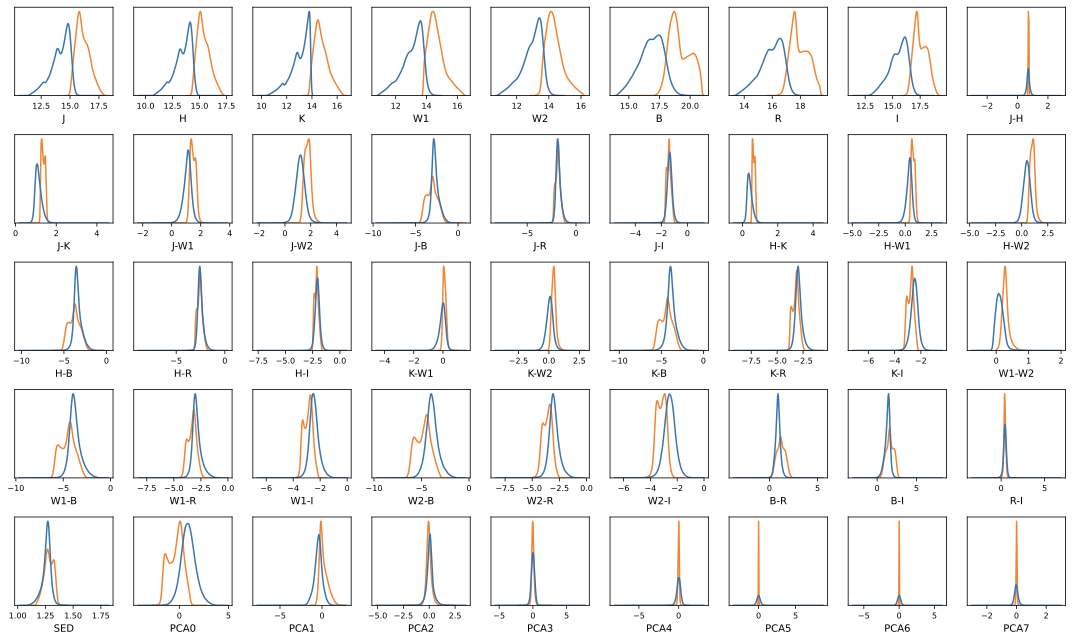
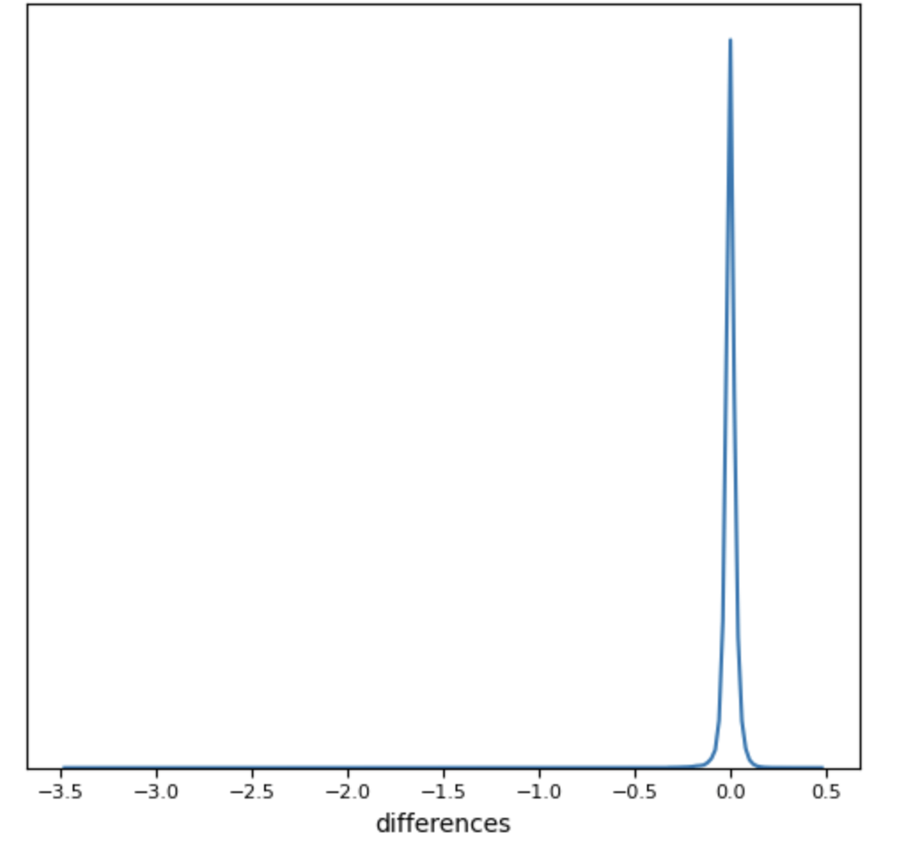
We noticed that the overall range of RMSE error tends to be from 0.0254 to 0.666 (Table 2): our RMSE tends to fall within the 0.0362–0.0379 range, which is on the lower side of RMSEs obtained by other models (Tables 2 and 3). Furthermore, the Gaussian KDE plots of the data and of the results (figures 3 and 4) revealed that there were positively skewed Gaussian distributions for the data (figure 3) and negatively skewed for the results (figure 4). These distributions were affected mostly due to the catastrophic outliers, which are defined as the data points with a predicted redshift which satisfies 

(8)  

From our results, we can see that our outliers (the data points which had an z>0.5 (figure 4)) make about 0.014% of the total testing dataset; about 6.08% of the catastrophic outliers are the normal outliers (which means that the rest of the catastrophic outliers had an z<0.5), and the catastrophic outliers were 0.23% of the entire testing dataset¹⁰. 

From Figure 4, we can see the z follows a standard gaussian distribution and that outliers are very easily definable as z>0.5 due to the symmetric nature of the distribution; furthermore, we can say that our predictions also follow a gaussian distribution of a similar nature. We can also see that our predictions were not very far off from the true redshift because the z<0.5; however, this could increase in higher redshift areas. Moreover, we can see from Figure 5 that the predictions did a good job of capturing a relationship between photometric and spectroscopic redshift (figure 5). From figure 5, we can see that most of the results are distributed tightly around a standard regression line. From the plot, we can see that from the linear regression model, we got a R² value of 0.881 and a regression line that matches the ideal line (y=x). Both of these facts tell us that our predictions have a strong correlation with the true redshift because the R² is close to 1 and that the regression line is basically the line y=x, which means that predicted redshift actual redshift.

 

Models:	RMSE
CWW31	0.0666
Bruzual-Charlot31	0.0552
Interpolated31	0.0451
Polynomial Regression31	0.0318
kNN31	0.0365
Kd-Tree31	0.0254
Bayesian31	0.0476
CWW LRG31	0.0473
Repaired LRG31	0.0476
ANNz (the RMSE between the photo-z and spec-z)	0.0371
LGBM training round 1 (refer to Table 1)	0.0362, which is a 2% decrease
Neural Network  training round 5 (refer to Table 1)	0.0375, which is a 1% increase

Discussion

Comparison of our results to the literature’s 

Collister and Lahav³³ utilized machine learning methods to predict the redshifts, which are calibrated towards the spec-z. They created an Artificial Neural Network (ANN) to predict the photometric data from the SDSS photometric data. The specific type of ANN they used is a basic MLPQNA (a multi-layer perceptron (MLP: a type of Feed-forward neural network) which uses a quasi-newton algorithm (QNA) to train and minimize the cost function of the algorithm): from now on, this model will be known as the ANNz model. Since its creation, it has been the state-of-the-art model in the literature for estimating and calibrating redshift predictions to spec-z. This model consists of many MLPQNAs. The structure of one MLP in the ANNz is 5:10:10:1, and the QNA is used to train the network. The SDSS photometric data, which they used for training, consists of magnitudes from five bands in a large sample and a smaller sample containing spectral data. Their training, validation, and testing sets consisted of 15000, 5000, and 10000 samples, respectively. The results of the ANNz compared with other methods that predict photometric redshift via the SDSS data are summarized in Table 3 (CWW (Coleman, Wu, and Weedman) and Bruzual-Charlot utilized the template method, and the interpolated method combines many different machine learning template-based techniques). Another method of estimating the photometric redshift is the Hyperz method (a template-based method), which, however, did overall worse than the ANNz on the SDSS data (greater RMSE dispersion and many systemic deviations in the results) because it had similar results to the algorithms in Table 3³³.

Csabai et. al.¹⁰ took their data from the SDSS to train multiple hybrid algorithms that combine both the template and machine learning-based techniques. Their data is split into two parts: the basic dataset and the Luminous Red Galaxy (LRG) dataset, which makes up the training set; they also added data from the 2-degree field survey (2df) and the Canada Network for Observational Cosmology (CNOC2) for the testing set. The main dataset consists of 27,797 galaxies, the average photometric redshift is 0.116, and the red-magnitude limit is 18. This dataset is only good for training the algorithms on redshift values up to 0.2. The LRG dataset consists of colors similar to those of an elliptical galaxy, 6698 galaxies, and an average photometric redshift of 0.227. This dataset is only good for training the algorithms on redshift values up to 0.5. The data from the 2df survey contains 5642 galaxies, a red-magnitude limit is 18.5, and the average photometric redshift of the data is 0.112. The data from the CNOC2 consists of a red magnitude of 21 and has an average photometric redshift value of 0.274, and it is only good for training the algorithms on redshift values up to 0.7¹⁰. 

The first technique that they implemented is fitting the polynomial regression on a training set that has more than 30,000 samples, 21 features, and a standard deviation of 0.027 of the redshift. Their second technique is fitting a kNN model, which is very uncommon in literature to use, and they decided to implement a Kd-tree to decrease the computation time and cost as the size of the training set increases: they found that error decreases as the size of the training set increases and the distance between neighbors decreases and the data must cover the appropriate range of the features of the testing samples. To solve this issue, they partitioned the n-dimensional feature space into equal-sized cells containing the training data using a Kd-tree and then fit a polynomial function on each cell: a method called 2d-Kd-tree partitioning of the training set.³⁴.  

This study aims to predict redshifts from WISE’s photometric data and calibrate those predictions to the spec-z. Our best result produced a 2% decrease from the RMSE of the ANNz; however, our worst result produced a 1% increase from the RMSE of the ANNz. 

(9)  

This percent change is probably small due to some conditions of the data, such as high photometric noise, which is typically inherent in this kind of data, or high uncertainties in the magnitude measures. Most of the studies in the literature have either used template-based spectrophotometric data or deep-learning algorithms trained on tabular photometry to estimate the redshift; however, our study’s simpler machine-learning algorithms have already obtained better results than the state-of-the-art ANNz, despite having a simpler architecture than the ANNz. 

We note that our best RMSE is 0.0362 (Table 1), and the best RMSE from the methods of Csabai et al. (2022)³⁴ is 0.0254 (Table 3), from the Kd-tree method, which was trained on the SDSS data (Table 3). They used a dataset that contained 34 000 samples from the Early Data Release; however, we used 1 073 261 galaxies in our training set. This makes our data set more complete and our methods more robust, as our analysis includes fainter galaxies and is not part of an early data release. Lastly, we note that the traditional machine learning methods tend to marginally outperform the state-of-the-art neural networks (Table 3). The traditional machine learning models achieve higher constraining power. At the same time, neural networks tend to perform marginally worse than their machine learning counterparts, potentially because the models are caught up in the noise due to their complex architecture (i.e., they transition into the overfitting regime). Furthermore, traditional machine learning models can extract and simplify the information given by features³⁴. 

In conclusion, despite having results only marginally better than the state-of-the-art, we did find that the traditional machine learning models do tend to do better in most scenarios than the complex deep neural networks, whether that was our results being 2% better than the ANNz or that was the results of the kNN outperforming all of the other methods as mentioned in Csabai et al. (Table 3)³⁴.

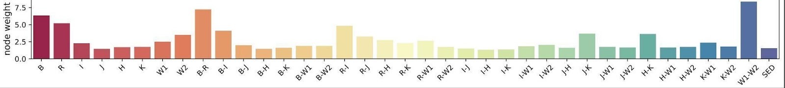
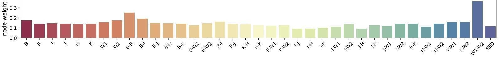
Analysis of Features

Along with producing better models, we were able to discern which features had the most importance, which can help future studies create even better models by training them on data that is highly focused on these features and discarding the ones with less importance and correlation (Figure 7). We note that they look qualitatively similar, with larger weights assigned to B, (B-R), and (W₁–W₂). These bar charts help us identify features of less importance, allowing us to discard them in subsequent analyses, to further simplify the models and the input data. The features of high importance are, as expected, since B and W₁–W₂ are on opposite sides of the spectrum of the different wavebands used, so most of the available information is captured by those filters. In addition, W₁ and W₂ are filters with very similar pass-through wavelengths, which allows the machine-learning model to pick up the slight brightness differences in that part of the spectrum. Furthermore, the same features that had a high correlation with the first main principal component have some of the highest importance values out of all the features, as seen in the Bottom graph (Figure 7).

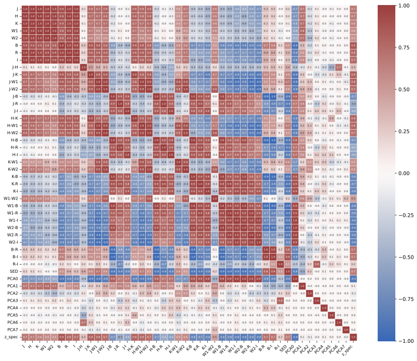
Figure 6 was created by plotting a heatmap of each feature and main component against each other,  where the colors represent Pearson’s correlation coefficient for a feature or main component (Figure 6). Pearson’s correlation coefficient is defined as

(10)  

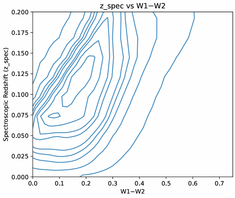
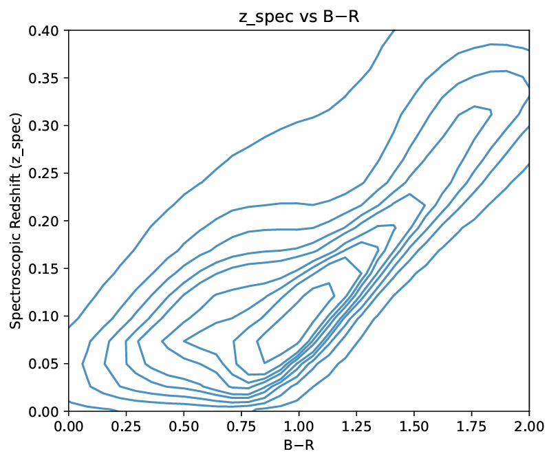
where x is the first feature that is being compared to the second feature y, x_i and y_i are the ith values of x and y, and y_mean and x_mean are the mean values of x and y. We determined an appropriate threshold value for Pearson’s correlation coefficient, for which if the absolute value of the correlation coefficient is higher for a certain feature than that threshold, then that feature would be considered an eigenvector of that component^19,35. Moreover, from figure 6, we can see that the features that have the most correlation with the first main component (PC_0) are all the colors involving the four magnitudes at the ends of the visible light and infrared spectrums (W₁, W₂, B, and R) and the colors which involve one of these four magnitudes and one of the middle magnitude (I, J, K, and H). While looking at the features closely correlated with the other principal components, we noticed that the W₁–W₂, B–R, B, and R features have the highest correlation with all four components, suggesting that they are key features and must have high predictive power with the models. We can also see the colors’ distributions through the two Gaussian KDE plots in Figure 8 ^{36,37,38,34,19,39} (Figures 6 and 8).

W₁ (3.4 m) and W₂ (4.6 m) are specific magnitudes that are used to measure the specific properties of galaxies. Since luminous galaxies are typically dust-filled (dust absorbs and emits infrared light (which is why we removed the galaxies in our plane as their light gets absorbed by the dust at the center of our galaxy)) and are old, their redshift is typically highly correlated with this color. Moreover, the B–R color traces newer stellar emissions⁴⁰. It was found by Bilicky et al.⁴¹, that fainter B or R magnitudes typically correspond to more distant objects, and the authors analyze the photometric redshift accuracy as a function of magnitudes and colours, showing that outliers and bias tend to increase at fainter magnitudes and extreme colours, confirming that magnitudes and colours are highly informative^40,41.

Cluver et al.⁴² found that since W₁ and W₂ probe the Rayleigh-Jeans trails of old stars, the W₁–W₂ color is sensitive to dust and age⁴². Moreover, Jarret et al.⁴³, Cluver et al.⁴², and Kauffman⁴⁴ that the color, W₁–W₂ is a strong tracer of mass which evolves with time, and that redder values of this color indicate that the galaxy is more massive, dusty, and dimmer, a phenomenon specifically associated with higher redshifts (which explains the 0.5 pearson correlation)^45,43,44. Bilicki et al.^46,41 and Krakowski et al.⁴⁷ have found that for machine learning, this color is extremely good for predicting redshift, especially for luminous galaxies for the same reasons^{46,48,49,50,51} 

As a galaxy’s spectral energy distribution (SED) is redshifted, its observed colors change because light originally emitted at shorter wavelengths shifts to longer wavelengths in the observer’s frame. The W1–W2 color, which normally samples mid-infrared light, begins to capture flux from rest-frame optical or even ultraviolet (UV) emission at higher redshifts. Similarly, the B–R color, which at low redshift primarily measures rest-frame optical light, progressively samples bluer rest-frame wavelengths as redshift increases. At sufficiently high redshift, the observed B and R bands no longer correspond to optical light but instead probe the galaxy’s rest-frame UV emission. For galaxies that are older, redder, or more dust-obscured (more common at higher redshifts) much of their emitted light is absorbed by dust and re-emitted at longer wavelengths, making the W1–W2 color redder as it becomes dominated by dust-reprocessed or redshifted stellar light^52,53,54.

Because both B–R and W1–W2 colors tend to increase (redden) with redshift—though influenced by galaxy type, dust content, and star formation history—they serve as useful proxies for estimating redshift and tracing galaxy evolution. Older galaxies, which are more prevalent at higher redshifts, tend to be intrinsically redder in both colors, reinforcing this correlation. Therefore, combining B–R and W1–W2 colors provides a broad yet effective representation of how galaxy colors evolve across redshift and various galaxy populations.^52,53,54

Future Considerations and Improvements

In the future, to obtain better results, researchers can implement some of the following methods to improve the computational power and accuracy of the models. For instance, Csabai et.al.³² found that, for estimating the photo-z, there is a more complex relationship between photometric data and the redshift, so they recommend using different types of regression functions for approximating bins of data instead of using one, simpler, regression function to try and capture the complex relationship between the data and photo-z³². Also, as utilized by Csabai et. al.³², implementing methods to reduce the computational processing time, such as the kd-tree and ball-tree, is beneficial because the models will be able to classify data as they are being observed^55,32. 

The data used to train future models should consider three things. The first is that the features of the data should be carefully picked based on past studies’ (such as this one) experiences. Magnitudes, fluxes, and colors are the standard features, but adding magnitude error, flux error, galactic coordinates, and galaxy shapes could make the models more robust. The second is that the database should be created by cross-matching data from various sources (as done in this paper and Bilicki et al.’s study). Lastly, the data and the features should be picked to minimize the signal-to-noise ratio^56,57,55,32.

Conclusion

Accurately estimating the redshift distribution and finding the optimal methods for accurate estimation is essential to advance the field of Cosmology and constrain the cosmological parameters. In this study, we aimed to do this by training traditional machine learning models. From reviewing the literature, we have seen that the neural networks, which are more complex models, reach the lowest error they can obtain (the ANNz) and produce noisier, less-interpretable results. We hypothesized that we can match state-of-the-art ANN models with traditional ML techniques, using precise feature engineering, to produce more interpretable results. We measure the interpretability of our models by the accuracy of our results (as they will be used for mapping the universe and for cosmological modeling) and the models’ algorithmic and computational simplicity. 

After training, our models’ RMSE errors fell within the 0.0362–0.0379 range. In the literature, the only models that have performed better than ours are the kd-tree, kNN, and polynomial regression models, which were, however, trained on an early-release SDSS data set, which was significantly data-limited. This reinforces the fact that traditional machine learning models’ estimates match the ANNz’s estimates (especially for data-limited situations), but an adequately sized training set and some degree of feature engineering are needed for the models to be useful. 

Furthermore, it is worth noting that our study serves as a proof-of-concept for cases where there is limited information on the accurate redshift of galaxies. Our models have been trained on low-redshift galaxies, and all of the models that have obtained a lower RMSE error than our models have also been trained on limited-data sources, which can be very useful to provide estimates of redshift for future cosmological surveys; however, many of them, such as the LSST and Euclid, will measure spectra systematically over a decade, thus partially eliminating the hindering factor of the limited availability of spectroscopic data to calculate the true cosmological redshift. Nevertheless, it should be noted once again that the redshift distribution of galaxies is the single largest nuisance source in state-of-the-art cosmological analyses, and it is important to develop optimal estimation methods for the near future.

Appendix

Github Code for this study: https://github.com/ksshah-29/Lumiere-Research-Project 

References

1. Aghanim, N., Y. Akrami, M. Ashdown, J. Aumont, C. Baccigalupi, M. Ballardini, A. J. Banday, R. B. Barreiro, N. Bartolo, S. Basak, R. Battye, K. Benabed, J. P. Bernard, M. Bersanelli, P. Bielewicz, J. J. Bock, J. R. Bond, J. Borrill, F. R. Bouchet, … A. Zonca. “Planck 2018 Results: VI. Cosmological Parameters.” Astronomy & Astrophysics, vol. 641, 2020, A6, https://doi.org/10.1051/0004-6361/201833910 [↩] [↩]
2. Bahcall, N. A., and P. Bode. “Hubble’s Law and the Expanding Universe.” Proceedings of the National Academy of Sciences, vol. 112, no. 1, 2015, pp. 63–66, https://doi.org/10.1073/pnas.1424299112 [↩]
3. Sánchez, C., Carrasco Kind, M., Lin, H., et al. “Photometric Redshift Analysis in the Dark Energy Survey Science Verification Data.” Monthly Notices of the Royal Astronomical Society, vol. 445, no. 2, 2014, pp. 1482–1506, https://doi.org/10.1093/mnras/stu1800 [↩] [↩] [↩] [↩]
4. Salvato, Mara, Olivier Ilbert, and Ben Hoyle. “The Many Flavors of Photometric Redshifts.” Nature Astronomy, vol. 3, no. 3, 2019, pp. 212–22, https://doi.org/10.1038/s41550-018-0478-0 [↩] [↩] [↩] [↩] [↩] [↩] [↩] [↩] [↩] [↩] [↩] [↩] [↩]
5. From Science Drivers to Reference Design and Anticipated Data Products.” The Astrophysical Journal, 2019 [↩]
6. “Overview of the Euclid Mission.” Astronomy & Astrophysics, 2025 [↩] [↩]
7. “The Sloan Digital Sky Survey: Technical Summary.” arXiv:astro-ph/0006396 [↩] [↩] [↩] [↩]
8. Norris, Ray, Mara Salvato, Giuseppe Longo, Massimo Brescia, T. Budavari, S. Carliles, Stefano Cavuoti, Duncan Farrah, J. Geach, K. Luken, A. Musaeva, Kai Polsterer, Giuseppe Riccio, N. Seymour, V. Smolčić, Mattia Vaccari, and P. Zinn. “A Comparison of Photometric Redshift Techniques for Large Radio Surveys.” Publications of the Astronomical Society of the Pacific, vol. 131, no. 1003, 2019, 108004, https://doi.org/10.1088/1538-3873/ab0f7b [↩] [↩] [↩] [↩] [↩] [↩] [↩] [↩] [↩] [↩] [↩]
9. “From Science Drivers to Reference Design and Anticipated Data Products.” The Astrophysical Journal, 2019 [↩]
10. Csabai, István, Tamas Budavári, Andrew Connolly, Alexander Szalay, Zsuzsanna Győry, Narciso Benítez, Jim Annis, Jon Brinkmann, Daniel Eisenstein, Masataka Fukugita, Jim Gunn, Suzannah Kent, Robert Lupton, Robert Nichol, and C. Stoughton. “The Application of Photometric Redshifts to the SDSS Early Data Release.” The Astronomical Journal, vol. 125, no. 2, 2003, pp. 580–92, https://doi.org/10.1086/345883 [↩] [↩] [↩] [↩] [↩] [↩] [↩] [↩] [↩] [↩] [↩] [↩] [↩]
11. Collister, Adrian, and Ofer Lahav. “ANNz: Estimating Photometric Redshifts Using Artificial Neural Networks.” Publications of the Astronomical Society of the Pacific, vol. 116, no. 818, 2004, pp. 345–51, https://doi.org/10.1086/383254 [↩] [↩] [↩] [↩] [↩] [↩] [↩] [↩] [↩] [↩] [↩] [↩]
12. Wright, E. L., Eisenhardt, P. R. M., Mainzer, A. K., Ressler, M. E., Cutri, R. M., Jarrett, T., Kirkpatrick, J. D., et al. “The Wide-field Infrared Survey Explorer (WISE): Mission Description and Initial On-orbit Performance.” The Astronomical Journal, vol. 140, no. 6, 2010, pp. 1868–1881, https://doi.org/10.1088/0004-6256/140/6/1868 [↩] [↩]
13. Hambly, N. C., MacGillivray, H. T., Read, M. A., Tritton, S. B., Thomson, E. B., Kelly, B. D., Morgan, D. H., Smith, R. E., Driver, S. P., Williamson, J., Parker, Q. A., Hawkins, M. R. S., Williams, P. M., & Lawrence, A. “The SuperCOSMOS Sky Survey – I. Introduction and Description.” Monthly Notices of the Royal Astronomical Society, vol. 326, no. 4, 2001, pp. 1279–1294, https://doi.org/10.1046/j.1365-8711.2001.04660.x [↩] [↩]
14. Bilicki, Maciej. “WISE × SuperCOSMOS Photometric Redshift Catalog: 20 Million Galaxies over 3π Steradians.” The Astrophysical Journal Supplement Series, vol. 225, no. 1, 2016, p. 24, https://doi.org/10.3847/0067-0049/225/1/5 [↩] [↩] [↩]
15. Zonca, A., L. P. Singer, D. Lenz, M. Reinecke, C. Rosset, E. Hivon, and K. M. Górski. “healpy: Equal Area Pixelization and Spherical Harmonics Transforms for Data on the Sphere in Python.” Journal of Open Source Software, vol. 4, no. 35, 2019, article 1298, https://doi.org/10.21105/joss.01298 [↩] [↩] [↩] [↩]
16. McInnes, Leland, John Healy, and James Melville. “UMAP: Uniform Manifold Approximation and Projection for Dimension Reduction.” 2018, arXiv:1802.03426 [↩] [↩] [↩] [↩]
17. Pedregosa, Fabian, Gaël Varoquaux, Alexandre Gramfort, Vincent Michel, Bertrand Thirion, Olivier Grisel, et al. “Scikit-learn: Machine Learning in Python.” Journal of Machine Learning Research, vol. 12, 2011, pp. 2825–30 [↩] [↩] [↩] [↩] [↩] [↩] [↩] [↩] [↩] [↩]
18. McInnes, Leland, John Healy, and James Melville. “UMAP: Uniform Manifold Approximation and Projection for Dimension Reduction.” 2018, arXiv:1802.03426 [↩]
19. Pedregosa, Fabian, Gaël Varoquaux, Alexandre Gramfort, Vincent Michel, Bertrand Thirion, Olivier Grisel, et al. “Scikit-learn: Machine Learning in Python.” Journal of Machine Learning Research, vol. 12, 2011, pp. 2825–30 [↩] [↩] [↩]
20. Abadi, Martín, Paul Barham, Jianmin Chen, Zhifeng Chen, Andy Davis, Jeffrey Dean, et al. “TensorFlow: A System for Large-Scale Machine Learning.” Proceedings of the 12th USENIX Symposium on Operating Systems Design and Implementation (OSDI ’16), 2016, pp. 265–83 [↩] [↩] [↩] [↩] [↩] [↩]
21. Bentley, Jon Louis. “Multidimensional Binary Search Trees Used for Associative Searching.” Communications of the ACM, vol. 18, no. 9, 1975, pp. 509–17 [↩]
22. Freund, Yoav, and Robert E. Schapire. “A Decision-Theoretic Generalization of On-Line Learning and an Application to Boosting.” Journal of Computer and System Sciences, vol. 55, no. 1, 1997, pp. 119–39 [↩] [↩]
23. Ke, Guolin, Qi Meng, Thomas Finley, Taifeng Wang, Wei Chen, Weidong Ma, Qiwei Ye, and Tie-Yan Liu. “LightGBM: A Highly Efficient Gradient Boosting Decision Tree.” NIPS ’17, 2017, pp. 3146–54 [↩] [↩]
24. Li, Lisha, Kevin Jamieson, Giulia DeSalvo, Afshin Rostamizadeh, and Ameet Talwalkar. “Hyperband: A Novel Bandit-Based Approach to Hyperparameter Optimization.” Journal of Machine Learning Research, vol. 18, 2018, pp. 1–52 [↩] [↩]
25. Jamieson, Kevin, and Ameet Talwalkar. “Non-Stochastic Best Arm Identification and Hyperparameter Optimization.” AISTATS 2016, 2016, pp. 240–48 [↩] [↩]
26. Firth, Andrew E., Ofer Lahav, and Rachel S. Somerville. “Estimating Photometric Redshifts with Artificial Neural Networks.” Monthly Notices of the Royal Astronomical Society, vol. 339, no. 4, 2003, pp. 1195–1202, https://doi.org/10.1046/j.1365-8711.2003.06271.x [↩] [↩] [↩]
27. Kiyani, E., M. Abdelkhalek, S. Bonnabel, and P. Ghaemi. “Machine-Learning-Based Data-Driven Discovery of Nonlinear Dynamic Systems.” Physical Review E, vol. 106, no. 6, 2022, 065303, https://doi.org/10.1103/PhysRevE.106.065303 [↩] [↩] [↩] [↩]
28. Kingma, Diederik P., and Jimmy Ba. “Adam: A Method for Stochastic Optimization.” ICLR ’15, 2015 [↩] [↩]
29. Nair, Vinod, and Geoffrey E. Hinton. “Rectified Linear Units Improve Restricted Boltzmann Machines.” ICML 2010, 2010, pp. 807–14 [↩]
30. Ramachandran, Prajit, Barret Zoph, and Quoc V. Le. “Searching for Activation Functions.” ICLR 2018, 2018 [↩]
31. “The Sloan Digital Sky Survey: Technical Summary.” arXiv:astro-ph/0006396. [↩] [↩] [↩] [↩] [↩] [↩] [↩] [↩] [↩]
32. Csabai, István, Tamas Budavári, Andrew Connolly, Alexander Szalay, Zsuzsanna Győry, Narciso Benítez, Jim Annis, Jon Brinkmann, Daniel Eisenstein, Masataka Fukugita, Jim Gunn, Suzannah Kent, Robert Lupton, Robert Nichol, and C. Stoughton. “The Application of Photometric Redshifts to the SDSS Early Data Release.” The Astronomical Journal, vol. 125, no. 2, 2003, pp. 580–92, https://doi.org/10.1086/345883 [↩] [↩] [↩] [↩] [↩] [↩]
33. Collister, Adrian, and Ofer Lahav. “ANNz: Estimating Photometric Redshifts Using Artificial Neural Networks.” Publications of the Astronomical Society of the Pacific, vol. 116, no. 818, 2004, pp. 345–51, https://doi.org/10.1086/38325 [↩] [↩]
34. Csabai, István, Tamas Budavári, Andrew Connolly, Alexander Szalay, Zsuzsanna Győry, Narciso Benítez, Jim Annis, Jon Brinkmann, Daniel Eisenstein, Masataka Fukugita, Jim Gunn, Suzannah Kent, Robert Lupton, Robert Nichol, and C. Stoughton. “The Application of Photometric Redshifts to the SDSS Early Data Release.” The Astronomical Journal, vol. 125, no. 2, 2003, pp. 580–92, https://doi.org/10.1086/345883 [↩] [↩] [↩] [↩] [↩]
35. Pearson, Karl. “Note on Regression and Inheritance in the Case of Two Parents.” Proceedings of the Royal Society of London, vol. 58, 1895, pp. 240–42 [↩]
36. Salvato, Mara, Olivier Ilbert, and Ben Hoyle. “The Many Flavors of Photometric Redshifts.” Nature Astronomy, vol. 3, no. 3, 2019, pp. 212–22, https://doi.org/10.1038/s41550-018-0478-0 [↩]
37. Norris, Ray, Mara Salvato, Giuseppe Longo, Massimo Brescia, T. Budavari, S. Carliles, Stefano Cavuoti, Duncan Farrah, J. Geach, K. Luken, A. Musaeva, Kai Polsterer, Giuseppe Riccio, N. Seymour, V. Smolčić, Mattia Vaccari, and P. Zinn. “A Comparison of Photometric Redshift Techniques for Large Radio Surveys.” Publications of the Astronomical Society of the Pacific, vol. 131, no. 1003, 2019, 108004, https://doi.org/10.1088/1538-3873/ab0f7b [↩]
38. Collister, Adrian, and Ofer Lahav. “ANNz: Estimating Photometric Redshifts Using Artificial Neural Networks.” Publications of the Astronomical Society of the Pacific, vol. 116, no. 818, 2004, pp. 345–51, https://doi.org/10.1086/383254 [↩]
39. son, Karl. “Note on Regression and Inheritance in the Case of Two Parents.” Proceedings of the Royal Society of London, vol. 58, 1895, pp. 240–42 [↩]
40. Bilicki, M., Jarrett, T. H., Peacock, J. A., Cluver, M. E., & Steward, L. “Mapping the Dark Universe with the Largest All‑Sky Surveys.” The Astrophysical Journal Supplement Series, vol. 210, no. 1, 2014, arXiv:1311.5246 [↩] [↩]
41. Bilicki, M., Jarrett, T. H., Peacock, J. A., et al. “Photometric Redshifts for the WISE × SuperCOSMOS All-Sky Galaxy Catalogue.” The Astrophysical Journal Supplement Series, vol. 225, no. 1, 2016, arXiv:1511.06570 [↩] [↩] [↩]
42. Cluver, M. E., Jarrett, T. H., Hopkins, A. M., et al. “Calibrating WISE W1 and W2 as Stellar Mass Indicators.” The Astrophysical Journal, vol. 782, no. 2, 2014, arXiv:1312.129 [↩] [↩] [↩]
43. Jarrett, T. H., Cluver, M. E., Magoulas, C., et al. “The WISE Extended Source Catalog (WXSC): Properties of Galaxies in the Mid‑Infrared.” The Astrophysical Journal, vol. 836, no. 2, 2017, arXiv:1709.02038 [↩] [↩]
44. Kauffmann, G. “The Physical Properties of Galaxies with Unusually Red Mid‑Infrared Colours.” Monthly Notices of the Royal Astronomical Society, vol. 470, no. 4, 2017 [↩] [↩]
45. Cluver, M. E., Jarrett, T. H., Hopkins, A. M., et al. “Calibrating WISE W1 and W2 as Stellar Mass Indicators.” The Astrophysical Journal, vol. 782, no. 2, 2014, arXiv:1312.1291 [↩]
46. Bilicki, M., Jarrett, T. H., Peacock, J. A., Cluver, M. E., & Steward, L. “Mapping the Dark Universe with the Largest All‑Sky Surveys.” The Astrophysical Journal Supplement Series, vol. 210, no. 1, 2014, arXiv:1311.5246. [↩] [↩]
47. Krakowski, T., Bilicki, M., Pollo, A., et al. “Photometric Redshifts for WISE × SuperCOSMOS Sources Using Machine Learning.” Astronomy & Astrophysics, vol. 596, 2016, A39, arXiv:1607.01020 [↩]
48. Bilicki, M., Jarrett, T. H., Peacock, J. A., et al. “Photometric Redshifts for the WISE × SuperCOSMOS All-Sky Galaxy Catalogue.” The Astrophysical Journal Supplement Series, vol. 225, no. 1, 2016, arXiv:1511.06570. [↩]
49. Cluver, M. E., Jarrett, T. H., Hopkins, A. M., et al. “Calibrating WISE W1 and W2 as Stellar Mass Indicators.” The Astrophysical Journal, vol. 782, no. 2, 2014, arXiv:1312.1291. [↩]
50. Jarrett, T. H., Cluver, M. E., Magoulas, C., et al. “The WISE Extended Source Catalog (WXSC): Properties of Galaxies in the Mid‑Infrared.” The Astrophysical Journal, vol. 836, no. 2, 2017, arXiv:1709.02038. [↩]
51. Kauffmann, G. “The Physical Properties of Galaxies with Unusually Red Mid‑Infrared Colours.” Monthly Notices of the Royal Astronomical Society, vol. 470, no. 4, 2017. Krakowski, T., Bilicki, M., Pollo, A., et al. “Photometric Redshifts for WISE × SuperCOSMOS Sources Using Machine Learning.” Astronomy & Astrophysics, vol. 596, 2016, A39, arXiv:1607.01020. [↩]
52. Wu, X.-B., Hao, G., Jia, Z., Zhang, Y., & Peng, N. “SDSS Quasars in the WISE Preliminary Data Release and Quasar Candidate Selection with Optical/Infrared Colors.” The Astronomical Journal, vol. 144, no. 2, 2012, p. 49, https://doi.org/10.1088/0004-6256/144/2/49 [↩] [↩]
53. Glowacki, M., Allison, J. R., Sadler, E. M., Moss, V. A., & Jarrett, T. H. “WISE Data as a Photometric Redshift Indicator for Radio AGN.” 2017, arXiv:1709.08634 [↩] [↩]
54. Wang, F., Wu, X.-B., Fan, X., Yang, J., Yi, W., Zuo, W., … Bian, F. “A Survey of Luminous High-Redshift Quasars with SDSS and WISE. I. Target Selection and Optical Spectroscopy.” The Astrophysical Journal, vol. 819, no. 1, 2016, p. 24 [↩] [↩]
55. Collister, Adrian, and Ofer Lahav. “ANNz: Estimating Photometric Redshifts Using Artificial Neural Networks.” Publications of the Astronomical Society of the Pacific, vol. 116, no. 818, 2004, pp. 345–51, https://doi.org/10.1086/383254 [↩] [↩]
56. Salvato, Mara, Olivier Ilbert, and Ben Hoyle. “The Many Flavors of Photometric Redshifts.” Nature Astronomy, vol. 3, no. 3, 2019, pp. 212–22, https://doi.org/10.1038/s41550-018-0478-0 [↩]
57. Norris, Ray, Mara Salvato, Giuseppe Longo, Massimo Brescia, T. Budavari, S. Carliles, Stefano Cavuoti, Duncan Farrah, J. Geach, K. Luken, A. Musaeva, Kai Polsterer, Giuseppe Riccio, N. Seymour, V. Smolčić, Mattia Vaccari, and P. Zinn. “A Comparison of Photometric Redshift Techniques for Large Radio Surveys.” Publications of the Astronomical Society of the Pacific, vol. 131, no. 1003, 2019, 108004, https://doi.org/10.1088/1538-3873/ab0f7b [↩]