
Abstract
Background and objective: Published studies of the Sun–Jupiter circular restricted three-body problem use slightly different mass parameters and do not all define the Jacobi constant in the same way, which makes their numbers awkward to compare. We ask whether the choice among published mass parameters changes anything qualitative about the Hill regions.
Methods: We collected five mass parameters from the literature and from JPL ephemerides and used interval arithmetic to enclose the collinear equilibria over the whole range they span, with an independent check in exact rational arithmetic. We also corrected a planar Lyapunov orbit near L1 and measured the small-oscillation frequencies near L4.
Results: Over the whole range, the critical Jacobi constants keep the same order, the gaps between them stay above 0.00127185, 0.0365307 and 0.00190647, the collinear points move monotonically with the mass parameter, and the triangular points remain linearly stable. Replacing the older value μ = 0.0009537 by the DE440 value moves L1 by about 3349 km, while the JPL solutions agree with one another to better than a kilometer.
Conclusions: The qualitative picture is the same for every mass parameter in use, and all of these shifts are small compared with the effect of ignoring Jupiter’s orbital eccentricity. The orbit and frequencies also serve as reference values for checking numerical codes.
Keywords: circular restricted three body problem; interval arithmetic; DE440; mass parameter sensitivity; periodic orbit verification
Introduction
A Lagrange point is a location where a negligible-mass object can remain stationary relative to two bodies in circular mutual motion. In rotating coordinates, the conserved Jacobi constant limits the speed available at each location, and where the implied squared speed would be negative, motion is impossible. The boundaries of these regions are zero-velocity curves, and the accessible regions they enclose are called Hill regions. As the Jacobi constant decreases, narrow necks open near the collinear Lagrange points. An open neck makes passage energetically possible, although it does not mean that any particular trajectory passes through it1,2.
The theory is old, but published numbers are not always easy to compare. The Sun–Jupiter mass ratio has been refined as planetary ephemerides and Juno radio tracking have improved3,4, so papers written at different times use different values. Some authors treat Jupiter alone as the secondary body and others the whole Jovian system, and some add a constant to the Jacobi constant while others do not2. When two published tables disagree in the fourth decimal place, it is not always obvious which of these choices is responsible.
Rigorous computer-assisted methods are well established for this problem. They have been used, for example, to prove the existence of heteroclinic connections and of Lyapunov orbits in the Sun–Jupiter system5,6, and libraries such as CAPD make such proofs practical7. Our use of interval arithmetic is much more modest, since it only encloses the roots of a scalar equation. We use it because it allows a single statement covering every published parameter value at once, instead of a separate check for each.
The question addressed here is therefore a narrow one: do the mass parameters found in the literature change the order in which the Hill-region necks open, or the linear stability of the equilibria? We compare five parameter values, record whether each source includes Jupiter’s satellites, and certify the result over an interval containing all of them. We also compute two quantities that are useful for testing restricted three-body codes: a planar Lyapunov orbit near L1 and the small-oscillation frequencies near L4. Throughout, we work with the planar circular model.
Methods
Model and Conventions
The primary and secondary are placed at (−μ, 0) and (1−μ, 0), with units chosen so that their separation and angular velocity are both one. With gravitational parameters G₁ and G₂, the mass parameter is μ = G₂/(G₁+G₂). For DE440 we use G₁ = 132712440041.279419 km³ s⁻² for the Sun and G₂ = 126712764.100000 km³ s⁻² for the Jovian system, that is, Jupiter together with its satellites8. This gives μ ≈ 0.000953881151935. Taking the mass ratio from DE440 does not, of course, make the circular model a substitute for the ephemeris itself3.
Let r₁ and r₂ be the distances to the two primaries. We use the potential and Jacobi constant without an additive shift:
(1) 
The equations of motion in the rotating frame are
(2) 
where r₁² = (x+μ)²+y² and r₂² = (x−1+μ)²+y². Some authors, including Koon et al.2, add μ(1−μ)/2 to Ω. The resulting shifted constant Cₛ satisfies
(3) 
and the same holds at L5. The shift changes the absolute values of the critical constants, but not the positions of the equilibria, their eigenvalues, the gaps between critical constants, or the Hill regions themselves. Before comparing published critical constants, it is therefore necessary to check which convention each source uses. We report both.
Historical Inputs and Interval Design
We use two values from the literature, μ = 0.0009537 (Koon et al. and Wilczak and Zgliczyński2,5) and μ = 0.00095387536 (Efthymiopoulos9), and three derived from JPL products: the DE405 header, the DE431 mass-parameter kernel and the DE440 table8,10,11. The second literature value is close to the DE440 ratio but is not a rounding of it. The exact numerical strings and the passages they come from are listed in Supplementary Note S2. All coordinates and constants in our tables were recomputed from these inputs rather than copied from the original papers.
The interval we certify runs from μ = 0.0009537 up to the DE405 ratio, approximately 0.000953881180363102, which is the largest of the five values. Both endpoints are taken from the exact decimal strings in the sources. The interval simply spans past modeling choices, and its width should not be read as an uncertainty in Jupiter’s mass.
The collinear equilibria are the roots of
(4) 
On each collision-free interval of the x-axis, F is continuous with Fₓ = 1+2(1−μ)/r₁³+2μ/r₂³ > 0 and changes sign between the ends of the interval, so L3, L1 and L2 exist and are unique. Supplementary Note S1 gives this standard argument together with the corresponding quintic equations. The triangular points lie at (1/2−μ, ±√3/2).
We divided the parameter interval into 256 subintervals and evaluated F in 100-digit decimal arithmetic with outward rounding. For each subinterval M and each collinear point we found a collision-free box [a, b] with sup F(a, M) < 0 and inf F(b, M) > 0, so that the box contains the root for every μ in M. Evaluating the relevant expressions over these boxes then bounds the critical constants and their differences. The derivatives with respect to μ follow from implicit differentiation:
(5) 
The derivatives of the three critical gaps turned out to have a fixed sign over the whole interval, so each gap takes its extreme values at the endpoints. We then tightened the final bounds using separate root enclosures at the two endpoints. As independent checks, we re-evaluated every recorded interval operation in exact rational arithmetic and repeated the computation with 70 digits and 128 subintervals, which gave the same signs. No binary floating-point arithmetic is used in this part of the calculation. The code itself has not been formally verified, so the result is a computer-assisted proof in the usual sense; Note S2 gives the details.
Independent Dynamical Checks
Linearizing about an equilibrium gives the characteristic equation
(6) 
At the triangular points the two frequencies satisfy
(7) 
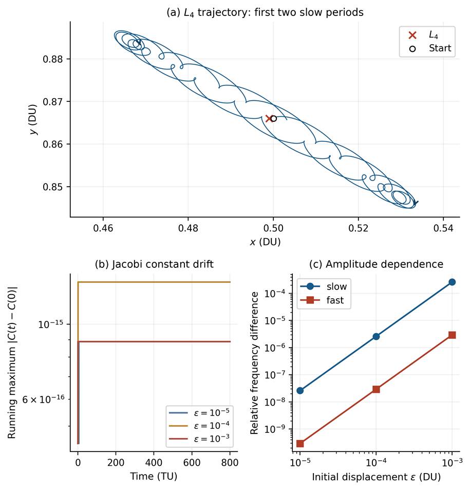
To test the integration near L4, we started orbits at x(0) = x₄+ε, y(0) = y₄ with zero velocity in the rotating frame, for ε = 10⁻⁵, 10⁻⁴ and 10⁻³, and integrated each one for 800 time units, or about ten slow periods. Both frequencies were estimated together by a least-squares harmonic fit to 4001 equally spaced samples, and we checked how much the estimates changed with the number of harmonics and the length of the fitting window. The integrations used DOP853, the explicit eighth-order Dormand–Prince method of Hairer, Nørsett and Wanner12, and were repeated at tighter tolerances. The periodic orbit was also integrated with the implicit Radau method for comparison. In these floating-point calculations the collinear points were located with Brent’s method13.
Equation (6) is unchanged if both Coriolis terms change sign, so matching frequencies does not show that the frame rotates in the right direction. We therefore also compared the rotating-frame acceleration, transformed to inertial coordinates, with the gravitational acceleration computed directly in the inertial frame, and compared the signed phase of the L4 oscillation with the linear solution.
For the planar Lyapunov orbit near L1, we fixed x(0) = x₁−0.001 and y(0) = vₓ(0) = 0 and adjusted vᵧ(0) by Newton iteration until vₓ vanished at the next crossing of y = 0, half a period later. The monodromy matrix was obtained by integrating dΦ/dt = A(t)Φ with Φ(0) = I over one full period. Unlike the equilibrium bounds, these orbit results are ordinary floating-point computations. Note S3 lists the event-detection settings, tolerances and fitting details.
Scale and Reproducibility
To express results in kilometers, we use a₀ = 5.20288700 au, the J2000 semimajor axis from JPL’s approximate planetary elements14, together with the IAU astronomical unit15. This nominal scale is used for illustration only and is independent of the DE440 mass ratio. Dimensionless values are given to enough digits for reproduction, and distances in kilometers are rounded to four significant figures. The study is purely computational and involved no human or animal subjects.
Results
Common-Convention Benchmarks
Table 1 compares L1 for the five inputs. The coordinates and Jacobi constants of all five equilibria in both conventions are given in Note S2 and in the accompanying data file. The two literature sources do not say whether Jupiter’s satellites are included, and the table labels them accordingly.
| Input | μ × 10⁴ | x₁ | Cₛ₁ | Secondary |
| Koon / Wilczak | 9.537000000 | 0.9323697524 | 3.0397090701 | Jupiter; satellites unspecified |
| Efthymiopoulos | 9.538753600 | 0.9323655873 | 3.0397138023 | Jupiter; satellites unspecified |
| DE405 | 9.538811804 | 0.9323654491 | 3.0397139593 | Jovian system |
| DE431 | 9.538811572 | 0.9323654496 | 3.0397139587 | Jovian system |
| DE440 | 9.538811519 | 0.9323654497 | 3.0397139585 | Jovian system |
For DE440 the shifted collinear constants are Cₛ₁ = 3.039713958548, Cₛ₂ = 3.038441863796 and Cₛ₃ = 3.001906833286, and Cₛ = 3 exactly at L4 and L5. Without the shift the corresponding values are 3.038760987286, 3.037488892533, 3.000953862024 and 2.999047028737. The offset between the two conventions, about 9.53 × 10⁻⁴, is much larger than any difference between the JPL inputs, so it is the first thing to check when published tables disagree.
With the nominal scale held fixed, replacing μ = 0.0009537 by the DE440 value moves L1 by −3349 km and L2 by +3373 km along the x-axis. Replacing the Efthymiopoulos value by DE440 moves them by −107.1 and +107.8 km, and replacing DE405 by DE440 moves them by only +0.5255 and −0.5292 km. These are differences between models at a fixed scale, not predicted changes in the real positions of the Lagrange points.
Parameter-Uniform Result
Proposition. For every μ in the interval defined above, C₁ > C₂ > C₃ > C₄ = C₅, dx₁/dμ < 0, dx₂/dμ > 0, dx₃/dμ < 0 and 27μ(1−μ) < 1. The collinear points are saddle–centers and the triangular points are linearly stable. In particular, the Hill-region necks open in the same order for all five parameter values.
Proof. Since Fₓ > 0, each collision-free interval contains exactly one root, and the interval sign conditions enclose it for every μ in each subinterval, including the shared endpoints. Evaluating Equation (5) on these enclosures gives the signs of the derivatives. The positive lower bounds in Table 2 give the order of the critical constants, and its last row gives Routh’s condition 27μ(1−μ) < 1. At each collinear point the enclosures give Ωxx > 0 and Ωyy < 0, while Ωxy = 0 by symmetry, so Equation (6), viewed as a quadratic in λ², has one positive and one negative root; this is the saddle–center case. C₄ = C₅ follows from the symmetry of the triangular points. Since the 256 subintervals cover the whole interval, these conclusions hold for every μ in it. The sequence of Hill regions then follows from the standard description of how the regions change as C passes each critical value, summarized in Note S1. ∎
| Quantity | Strict lower bound | Strict upper bound |
| C₁ − C₂ | 0.00127185 | 0.00127210 |
| C₂ − C₃ | 0.0365307 | 0.0365351 |
| C₃ − C₄ | 0.00190647 | 0.00190684 |
| 27μ(1−μ) | 0.02572533 | 0.025730230 |
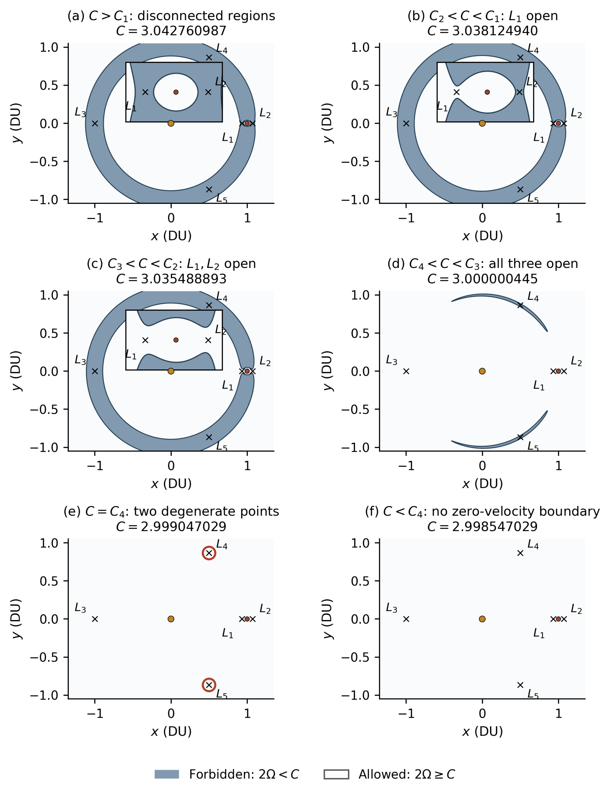
The derivative enclosures are −23.754 < dx₁/dμ < −23.750, 23.918 < dx₂/dμ < 23.922 and −0.416667 < dx₃/dμ < −0.416666. Note S1 also shows that 2Ω ≥ C₄ everywhere, with equality only at L4 and L5. Table 3 lists the six regimes of the Hill region as C decreases, and Figure 1 shows each of them. In panels (a)–(d) we used values of C between the critical levels so that the necks have visible width.
| Range | Geometric change | Figure 1 |
| C > C₁ | Three allowed components; both primary lobes isolated from exterior. | (a) |
| C₂ < C < C₁ | L1 neck connects primary lobes; exterior remains separate. | (b) |
| C₃ < C < C₂ | L2 neck connects the interior to exterior. | (c) |
| C₄ < C < C₃ | L3 passage also opens; two forbidden regions remain. | (d) |
| C = C₄ = C₅ | No forbidden area; zero-velocity locus reduces to L4 and L5. | (e) |
| C < C₄ | Entire collision-free plane allowed; zero-velocity locus empty. | (f) |
Orbit and Frequency Verification
The corrected L1 orbit starts at (x, y, vₓ, vᵧ) = (0.931365449731, 0, 0, 0.00742833322210) and has period 2.88599403264 and Jacobi constant C = 3.038715607033. Five Newton iterations reduced the closure error after one period below 2 × 10⁻¹³ in the Euclidean norm of the state, and the Radau trajectory agrees with the DOP853 one to within 4 × 10⁻¹². The monodromy matrix has the hyperbolic pair of multipliers 2283.76525 and 0.000437873375, and the remaining two multipliers equal one to numerical precision, as expected for a periodic orbit of an autonomous Hamiltonian system. The product of the hyperbolic pair differs from one by less than 5 × 10⁻¹⁰ and the symplectic residual is below 2 × 10⁻⁹, so only the leading digits of the multipliers are reliable. Closure was computed from the unrounded initial state given in the data file, and Figure S2 compares results at different tolerances.
At L4, Equation (7) gives ωs = 0.0804641214931 and ωf = 0.996757505692, corresponding to periods 78.08679434 and 6.303624775. For ε = 10⁻⁵ the fitted frequencies differ from these values by 2.60 × 10⁻⁸ and 2.93 × 10⁻¹⁰ in relative terms. Each tenfold increase in ε makes these differences about a hundred times larger (Figure 2c). This quadratic dependence on amplitude is what the leading nonlinear terms predict16, so the differences reflect the dynamics rather than integration error.
In the sign test, the correct equations reproduce the inertial acceleration to within 4.5 × 10⁻¹⁶ at the sampled points, whereas reversing both Coriolis terms produces errors larger than 0.083. The signed phase comparison also rejects the reversed equations. Neither Jacobi conservation nor the frequencies alone would have revealed this kind of error.
Discussion
The equilibria, Routh’s criterion and the sequence of Hill regions are textbook material1. What this paper adds is a check, with explicit bounds, that the qualitative picture is the same for every mass parameter used in the Sun–Jupiter literature, together with a set of reference values for testing code. The rigorous studies cited in the Introduction answer much harder questions about orbits and transport, which we do not address here.
For the planar problem, nonlinear stability of the triangular points is already known. Deprit and Deprit-Bartholomé17 proved Lyapunov stability for all μ below the Routh value except at three special values, approximately 0.024293, 0.013516 and 0.010914, where their criterion does not decide the question. All five Sun–Jupiter values lie far from these, so their theorem applies to every case studied here. Our integrations are consistent with this result, but since they cover a finite time they do not prove it, and they say nothing about the spatial problem or the real Solar System.
The main physical limitation is the assumption of a circular orbit. With Jupiter’s eccentricity e = 0.04838624 from the same element set, the Sun–Jupiter distance varies by ±a₀e ≈ ±3.766 × 10⁷ km. Scaling the distance from Jupiter to L1 by the same factor gives about ±2.511 × 10⁶ km. This is only a rough indication, because the elliptic problem is time-dependent and allows behavior, such as global instability, that the circular model cannot show18. Even so, it is several orders of magnitude larger than the differences between mass parameters in Table 1, which are in turn much larger than the numerical error in the computed roots.
The frequency estimates depend slightly on the fitting window, the number of harmonics and the amplitude, and Note S3 reports the size of these variations. The figures are illustrations only, and the statements about the Hill regions rest on the proposition rather than on the plotted contours.
Conclusion
For all five Sun–Jupiter mass parameters considered, the critical Jacobi constants occur in the same order, the gaps between them are bounded well away from zero, and the equilibria have the same stability type. When published values disagree, the Jacobi convention should be checked first, because its offset of about 9.53 × 10⁻⁴ is larger than the effect of any of the mass-parameter changes. The JPL solutions themselves agree to well under a kilometer in the position of L1. The L1 orbit, the L4 frequencies and the Coriolis sign test give simple benchmarks for checking restricted three-body codes. A natural extension is the elliptic problem, where Jupiter’s eccentricity outweighs all of the effects considered here.
Data and Code Availability
The Supporting Information contains Notes S1–S3, the analysis code, the interval certificates and their rational re-evaluation, the numerical tables and figures, snapshots of the JPL source files with checksums, and instructions for reproducing the results. This work received no external funding.
Supplementary Material
References
- V. Szebehely. Theory of orbits: the restricted problem of three bodies. Academic Press, 1967, https://doi.org/10.1016/B978-0-12-395732-0.X5001-6. [↩] [↩]
- W. S. Koon, M. W. Lo, J. E. Marsden, S. D. Ross. Heteroclinic connections between periodic orbits and resonance transitions in celestial mechanics. Chaos: An Interdisciplinary Journal of Nonlinear Science. Vol. 10, pg. 427–469, 2000, https://doi.org/10.1063/1.166509. [↩] [↩] [↩] [↩]
- R. S. Park, W. M. Folkner, J. G. Williams, D. H. Boggs. The JPL planetary and lunar ephemerides DE440 and DE441. The Astronomical Journal. Vol. 161, pg. 105, 2021, https://doi.org/10.3847/1538-3881/abd414. [↩] [↩]
- V. Notaro, D. Durante, L. Iess, S. J. Bolton. Determination of Jupiter’s mass from Juno radio tracking data. Journal of Guidance, Control, and Dynamics. Vol. 44, pg. 1062–1067, 2021, https://doi.org/10.2514/1.g005311. [↩]
- D. Wilczak, P. Zgliczyński. Heteroclinic connections between periodic orbits in planar restricted circular three-body problem – a computer assisted proof. Communications in Mathematical Physics. Vol. 234, pg. 37–75, 2003, https://doi.org/10.1007/s00220-002-0709-0. [↩] [↩]
- M. J. Capiński. Computer assisted existence proofs of Lyapunov orbits at L2 and transversal intersections of invariant manifolds in the Jupiter–Sun PCR3BP. SIAM Journal on Applied Dynamical Systems. Vol. 11, pg. 1723–1753, 2012, https://doi.org/10.1137/110847366. [↩]
- T. Kapela, M. Mrozek, D. Wilczak, P. Zgliczyński. CAPD::DynSys: a flexible C++ toolbox for rigorous numerical analysis of dynamical systems. Communications in Nonlinear Science and Numerical Simulation. Vol. 101, pg. 105578, 2021, https://doi.org/10.1016/j.cnsns.2020.105578. [↩]
- NASA Jet Propulsion Laboratory. Astrodynamic parameters, DE440 planetary-system gravitational parameters. https://ssd.jpl.nasa.gov/astro_par.html, n.d. Accessed 16 September 2026; source snapshot in Supporting Information. [↩] [↩]
- C. Efthymiopoulos. Nekhoroshev stability estimates for different models of the Trojan asteroids. Proceedings of the International Astronomical Union. Vol. 2004(IAUC197), pg. 195–204, 2004, https://doi.org/10.1017/s1743921304008658. [↩]
- NASA Jet Propulsion Laboratory. DE405 ASCII ephemeris header, header.405, groups 1040 and 1041. https://ssd.jpl.nasa.gov/ftp/eph/planets/ascii/de405/header.405, n.d. Accessed 16 September 2026. [↩]
- NASA Jet Propulsion Laboratory. DE431 mass-parameter kernel, gm_de431.tpc. https://naif.jpl.nasa.gov/pub/naif/generic_kernels/pck/gm_de431.tpc, 2014. Last modified 8 January 2014; accessed 16 September 2026. [↩]
- E. Hairer, S. P. Nørsett, G. Wanner. Solving ordinary differential equations I: nonstiff problems. 2nd ed. Springer, 1993, https://doi.org/10.1007/978-3-540-78862-1. [↩]
- R. P. Brent. An algorithm with guaranteed convergence for finding a zero of a function. The Computer Journal. Vol. 14, pg. 422–425, 1971, https://doi.org/10.1093/comjnl/14.4.422. [↩]
- NASA Jet Propulsion Laboratory. Approximate positions of the planets, 1800–2050 element fit and nominal errors. https://ssd.jpl.nasa.gov/planets/approx_pos.html, n.d. Accessed 16 September 2026; source snapshot in Supporting Information. [↩]
- International Astronomical Union. Resolution B2 on the re-definition of the astronomical unit of length. XXVIII General Assembly, 2012, https://iauarchive.eso.org/static/resolutions/IAU2012_English.pdf. [↩]
- R. I. Páez, U. Locatelli, C. Efthymiopoulos. New Hamiltonian expansions adapted to the Trojan problem. Celestial Mechanics and Dynamical Astronomy. Vol. 126, pg. 519–541, 2016, https://doi.org/10.1007/s10569-016-9710-3. [↩]
- A. Deprit, A. Deprit-Bartholomé. Stability of the triangular Lagrangian points. The Astronomical Journal. Vol. 72, pg. 173–179, 1967, https://doi.org/10.1086/110213. [↩]
- A. Delshams, V. Kaloshin, A. de la Rosa, T. M. Seara. Global instability in the restricted planar elliptic three body problem. Communications in Mathematical Physics. Vol. 366, pg. 1173–1228, 2019, https://doi.org/10.1007/s00220-018-3248-z. [↩]