

Abstract
Predicting cotton yield is important in agriculture because of its wide use in clothing production. Cotton is a commodity that is extremely climate sensitive and requires specific locations to grow. Traditionally, non-spatial models have been used with climate, infield, and geographic data to predict cotton yield. Spatial models use spatial data patterns in their predictions that aren’t used in non-spatial models. Therefore, we hypothesized that GM Lag, an autoregressive spatial model, would predict cotton yield better than non-spatial models. Along with GM Lag, we chose to use Linear Regression, KNN Regression, Random Forest Regression, and Neural Networks because they were non-spatial models with varying complexities. Through this study, we found that there are minimal spatial relationships to assist GM Lag at the state-wide level based on a Global Moran’s I of +0.10 with a pseudo-p-value of 0.14. Furthermore, we found that GM Lag achieved a lower MSE than Linear Regression when it was predicting seen states but had a higher MSE when predicting unseen states. Additionally, this research describes how geospatial data can be used differently to possibly better predict cotton yield.
Keywords: cotton yield prediction, spatial regression, machine learning, geospatial data.
Introduction
Cotton is an essential commodity in the modern world, with it being one of the most important fiber crops worldwide1. More than 100 countries produce cotton over 33.2 million hectares with an average annual cotton production of 18.9 million tons2.
Cotton is a crop that is particularly sensitive to climate3,4, and, as a result, climate change and rising temperatures will drastically affect its yield. Cotton requires an annual rainfall of 500-1500 millimeters. Temperatures of 20° to 30° C facilitate optimal cotton growth5. The sensitivity of cotton to climatic conditions suggests that accurate, data-driven predictions can help farmers make more informed decisions regarding planting and harvesting.
We intend to determine if using spatial relationships, through geospatial data, in GM Lag improves the accuracy of cotton yield predictions compared to non-spatial models that don’t consider these patterns6. Additionally, this study aimed to use geospatial, temporal, and climate data to predict state-wide cotton, explore the significance of climate versus state data in predicting cotton yield, and identify state cotton yield hotspots.
Machine Learning models are popular in making predictions because they can identify complex data patterns that humans cannot. We chose to use multiple contrasting models because certain machine learning algorithms work better than others depending on the problem. Through a process of comparing each model’s result with metrics, we can identify which model performs better.
We compared the results of five models: Linear Regression, KNN Regression, Random Forest Regression, Dense Neural Network, and GM Lag. These models were contrastingly different, with varying complexities. We chose to use Linear Regression because it is a simple model that is often used for predictive problems with linear trends7. We chose to use KNN Regression because originally it is a classification model that is also versatile for numerical problems8. We chose to use a Random Forest regression because it is an ensemble model that uses complex questions to efficiently adapt9. We chose to use a Dense Neural Network because it is an extremely complex model that may see nonlinear patterns that simpler models don’t10. Random Forest and Neural Networks have an advantage over Linear Regression because they are more adaptable and robust models compared to Linear Regression through more weights and complex questions. The models used are discussed more in the Methods Section.
Generalized Methods of Moments Estimation (GM Lag) is a spatial linear model that uses yield values of neighboring states in predictions. Normally, Linear Regression works by calculating the weights for each feature that minimizes the sum squared error of every datapoint. GM Lag is similar to Linear Regression because it uses a line of best fit for predictions. However, GM Lag uses a spatial weight matrix when determining its feature coefficients and weights6.
Using geospatial data refers to a specific location, which in our case is state geometry shapes11. In this study, our models will incorporate specific state geometries to predict cotton yield. Non-spatial models refer to models that do not take geospatial data into account in their algorithms.
Autocorrelation refers to the correlation between values of a variable at different locations within a geographic space. Autocorrelation discovers if values of a sample are similar or different to other samples in its geographic proximity. In geospatial analysis, this concept can help identify spatial patterns. Statistical measures such as Moran’s I show if there is autocorrelation12.
We used choropleth maps as our main type of graph. Choropleth mapping uses different shades of colors and geographic boundaries to show a certain quality or value in a graph13. For example, choropleth mapping is used to display Local Moran’s I hotspots.
For this study, we used three approaches to analyze relationships between cotton yield and different types of data. These approaches changed what data was included in the dataset when training the model. Approach 1 was training our model with weather and year data. Approach 2 was training our model with state and year data. Approach 3 was training our model with weather, state, and year data. Based on these approaches, model accuracy was compared to explore what data was helping and hurting the model. The approaches used are discussed more in the Methods Section.
Mean Squared Error (MSE), Mean Absolute Error (MAE), R2 Score, and Bootstrap Confidence Intervals were the four model metrics used in this study. MSE and MAE are error metrics while R2 Score is a correlation metric14. Bootstrap Confidence Intervals are statistical tests that give an interval of where a distribution is within a chosen confidence interval to test statistical significance. The metrics are discussed more in the Methods Section.
We used three statistical autocorrelation measures, which are Global and Local Moran’s I, and p-value. There are two types of Moran’s I measures: Global Moran’s I and Local Moran’s I. Global Moran’s I is a scalar that shows overall autocorrelation strength and Local Moran’s I detects hotspots of autocorrelation15. P-value measures the probability that the null hypothesis is true. The null hypothesis assumes that an independent variable has no effect on the outcome. P-values determine if the features are related to the outcome and are also used in autocorrelation. Lower p-values under 0.05 indicate that the autocorrelation relationships found are not by chance16.
In the past, papers have used non-spatial models with only climate parameters to predict cotton yield in Brazil, however the R2 score was relatively low5. Their highest performing model was Random Forest Regressors with an R2 adjusted score of 0.38, followed by a variety of models such as Multiple Linear Regression, K Neighbors Regressor, Multi-layer Perceptron and Gradient Boosting. Additionally, it was found that evapotranspiration and water storage were the two parameters that most positively correlated to cotton production. Although they had coordinates of data points in their dataset, they chose not to use geospatial models. To build on to this paper, GM Lag with climate parameters will be used. Additionally, our study will not be restricted to specifically climate data since geospatial, temporal, and state data will be incorporated.
In a paper predicting within-field cotton yields using publicly available datasets, similar models were used such as Random Forest Regression and Gradient Boosting Machines1. This paper’s main focus was using infield data, such as soil properties, to observe and predict how cotton yield predictions change depending on the stages of cotton growth (Squaring, Flowering and Boll-fill). However, this paper used both soil property data as well as one climatic parameter of rainfall. Random Forest had a highest R2 score of 0.48 and GBM had a highest R2 score of 0.7. The data used were from 2 irrigated paddocks on an Australian farm from 2014 – 2016. Since the amount of data, 2 years on 2 separate farms, was so low, we chose to use a wider and broader dataset. Differentiating from this paper, we chose to focus on more climatic and geographic data rather than soil property data.
In summary, we hypothesized that incorporating spatial relationships through a spatial weight matrix in GM Lag would lead to more accurate predictions than non-spatial models, due to an expected positive autocorrelation in cotton yield. In our approach, we tested the presence or absence of geospatial data in each model and assessed performance. Our dataset achieved a global Moran’s I of +0.10 with a pseudo p-value of 0.14, which shows weakly positive and statistically insignificant autocorrelation to cotton yield.
Methods
Dataset
We used a public dataset found on Kaggle with many climate parameters, specific US states, years, and corresponding cotton yield. This dataset was created by Abhirup Saha, a researcher at Penn State17.
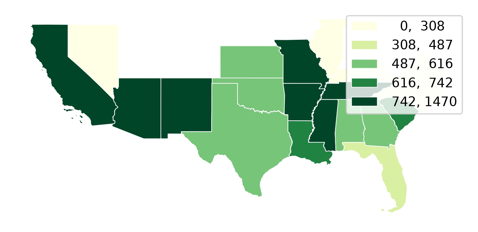
The dataset had 28 features with 528 samples (Appendix A). For our models, the data had to be numerical. Most of the data (climate parameters) was numerical other than the states. Performing geospatial analysis requires more data about the state beyond the state name, so a US Census dataset with state names, geometry of states, and coordinates were merged (Figure 1). The climate parameters included features of average temperature, maximum temperature, precipitation, PDSI, PHDI, and PMDI. PDSI and PMDI describe drought severity, while PHDI describes water supply in reservoirs and groundwater. Extended variable descriptions are found in Appendix A.
Data Pre-processing
With the first step in data pre-processing, the dataset contained temporal data, ranging from 1975 – 2002. We chose to use all the data across the years and enumerated them into integers (0, 1, 2, 3…). To express state data, each sample was appended with a latitude and longitude of the center of the state. One hot encoding was not used because when doing the Leave One Group Out approaches, the model would not adjust the weight to that one hot encoding and the predictions would inflate massively.
Missing data was imputed using the mean values of available data. However, since analyzing geographic patterns was a main focus, the samples without states names were dropped.
Linear or Quadratic Years
Since the dataset spans critical years of climate change (1975-2002), simply encoding years as linear terms may not sufficiently capture the correlation years have on cotton yield. Therefore, we tested a full dataset with linear years and another full dataset with a linear year column and a year squared column. Since adding a non-linear term would most strongly affect Linear regression models which could not capture non-linear relationships initially, we plotted the residuals of both datasets. Furthermore, we supplemented this with a nested F-test on OLS and documented the P-value. A nested F-test is used to check if adding new variables improves model results enough to be significant. If the p-value found was above 0.05, linear years would be used.
Cross Validation Techniques
We used different cross validation techniques that alter what data is in training and testing sets.
K-Fold Cross Validation
K-Fold Cross Validation is a technique used to determine how well a machine learning model generalizes and determines standard deviation. The dataset is split into k folds where k is a hyperparameter chosen. A model is trained on k-1 folds and evaluated on the held out fold. This is done k times to determine the mean error value and the standard deviation18. K-Fold Cross Validation is used to avoid having a training test split that is not representative of the entire dataset in order to get meaningful results. We used K = 5 folds.
Time Series Cross Validation
Time Series is a technique used in time series prediction to ensure that models aren’t using future year datapoints to predict past years, which is data leakage. Time series involves splitting datasets into testing sets where samples are only from a single year and training sets where samples are only from years previous. We used a sliding window of 10 years for our training data to keep the training sizes constant. As a result, we started predictions at Year 10.
Group K Fold
Group K Fold Cross Validation is a technique that splits testing sets to only include specific groups, leaving these groups out of the training set. Group KFold is used when samples have related features. Group KFold Groups were set by state to test how well models could generalize to new states. Furthermore, GroupKFold is used in addition to LOGO because it provides more stable results. We used K=5 groups.
Leave One Group Out Cross Validation
Leave One Group out (LOGO) cross validation is a technique to test how well models would generalize to predicting new states. LOGO creates a testing set of all samples that are of a unique group. The remaining dataset comprised of all other groups becomes the training set. Our groups were unique states.
Approach 1: Testing with Climate and Year Data (Reduced Dataset)
The first baseline approach involved dropping all state information, which left all columns with climate data and temporal data (26+ columns). Approach 1 was created to compare it with Approach 2 and 3. This approach was used to ask if climate and year data could provide enough information to better predict cotton yield over geographic data.
Approach 2: Testing with State and Year Data (Reduced Dataset)
The 2nd baseline approach involved dropping all variables besides Year and State information. Approach 2 was created to compare with Approach 1 and 3. This approach was used to ask if state and year data could provide enough information to better predict cotton yield over climatic data.
Approach 3: Testing with Climate, Year, and State Data (Full Dataset)
The 3rd approach involved testing models with our combined dataset: climate, year, and state coordinates. Approach 3 was created to compare it with Approach 1 and 2. This approach was used to ask if using state, weather, and year data would best predict state-wide cotton yield.
Models Used
5 models (4 non-spatial + GM Lag) were chosen: Linear Regression, KNN Regressor, Dense Neural Network, Random Forest Model, and GM Lag.
Linear Regression
Linear Regression was chosen because it is a baseline model from its simplicity, which could be compared to other models19. Linear Regression computes a line of best fit between the multiple X features and y value with coefficients and weights7.
KNN Regression
KNearest Neighbors (KNN) is normally a classification model that uses nearby and similar data points for predictions. Based on how far these data points are, it makes a prediction20. However, KNN Regression is a modified version of this commonly used classification model to apply it to regression problems8. This classification model used for regression was chosen to see if classification models are better for predicting cotton yield. We performed a tuning step on all k values from k=2 to k=50 on a full dataset to find the optimal K value. As a result, we found that the optimal k value was 5, which was used for all KNN Regression models.
Random Forest Regression
Random Forest Regression was chosen because it is a robust algorithm that performs well in regression applications9. At the core, Random Forest models are many Decision Trees. Decision Trees are similar to flow charts, where each numerical data feature is put in a node and travels down computing branches to produce a prediction. A Random Forest model works by merging many decision trees together to produce a prediction21. We used SciKitLearn’s randomized search cv to search 100 different parameter combinations to find the optimal parameters of a full dataset. Our optimal parameters were {n_estimators = 700, min_samples_leaf = 12, max_features = ‘sqrt’, max_depth = 12, random_state = 42}. This was used for all random forest models.
Neural Networks
Neural Networks are a model algorithm inspired by the human brain. The neural network input layer has nodes and neurons for each independent feature. In the hidden layer, the network applies weights to determine an output. Neural Networks are commonly used for deep learning problems, such as detecting objects in images10. Nonetheless, Neural Networks can also be used for numerical regression problems22. In our case, we wanted to find if these deep learning algorithms would perform well in this numerical problem. For our Neural Network architecture, we used 5 layers, 3 hidden layers and an input and output layer. We used an Adam Optimizer with a learning rate of 0.0001. The first hidden layer consists of 128 neurons with a ReLU activation function, followed by a batch normalization layer and a 20% dropout layer. The second hidden layer consists of 64 neurons with a ReLU activation function, batch normalization, and a 20% dropout. Third hidden layer had 32 neurons with a ReLU activation function and a 10% dropout function. Finally, this was mapped to the one output neuron with a linear activation function. 32 Epochs were used with a batch size of 32. ReLU was used to create nonlinearity in the function. To prevent overfitting, dropout and early stopping were used. Early stopping was determined by plotting training and validation loss of each epoch and stopping when validation loss was higher than training loss.
Spatial Autoregressive Model
PYSALs SPREG (Spatial Regression) GM_Lag model was used to perform our spatial regression. GM Lag is a Spatial Autoregressive Model estimator, meaning it adds a weighted average of neighboring state yield values in its predictions. This model creates a spatial matrix in its predictions.~The spatial matrix is a series of weights that describes what samples from the training dataset are neighbors to the sample. The model multiplies the weight matrix by the neighboring samples dependent variable/cotton yield and adds this after multiplying it by a coefficient  . For row standardization, the samples of the matrix that are neighbors are filled with 1/n, where n is the number of neighbors. This model finds the average weight of all of its neighbors and adds it to a Linear Regression model that takes in the other input features. This model assumes that there are stronger relationships and similarities with datapoints geographically closer than datapoints that are farther away.~A Queen Contiguity weight matrix was used, which counts neighbors as any sample that has a geometry object that shares any edge or vertex. Generalized Methods of Moments estimation refers to the method of estimating the coefficients.
SPREG GM Lag doesn’t have an out of sample inference method that utilizes spatial weights in its predictions. As a result, for predictions, we created a method that fits a GM Lag model to the training data and creates a Queen weight matrix on these training samples. In inference, the model finds neighbors of the testing sample in the training set and creates a weight matrix for prediction. Since state geometries are shared, the Queen Contiguity Weight Matrix counts own states as neighbors in predictions, as well as neighboring states. As a result, this repurposed inference method of GM Lag depends also on own state yield, which lowers clarity on how much neighboring states improve GM Lag. The equation of Spatial Autoregression is listed below, with Wy representing the weight matrix,  representing the model coefficients,
 representing the input features, and
 representing the bias.
Spatial Autocorrelation Measures
Multiple spatial autocorrelation methodologies were used to explore spatial relationships in our dataset along with supporting the results from GM Lag, such as Global and Local Moran’s I and p-score. Moran’s I is a statistical measure used to interpret autocorrelation. Global Moran’s I is a number ranging from -1 to 1 that interprets if and how strong an autocorrelation relationship is. Negative values show a negative correlation while positive values show a positive correlation. Since the dataset contained samples of the same state from multiple years, performing Global Moran’s I on all 528 samples would overinflate the spatial relationships. As a result, we collapsed all state yields across yields by averaging state yield across years for each state. Across the 20 states, years of data per state ranged from 24 to 28, which slightly imbalances average across years. We used a queen contiguity weight matrix with row standardized weights. The number of permutations to calculate the pseudo p-value was 9999 with the random seed being 42. The coordinate reference system used was EPSG:4269.
Local Moran’s I is an array of numbers showing how strong an autocorrelation is relating to neighboring states. In other words, Local Moran’s I shows hotspots15. Local Moran’s I can be shown through graphs. Our Local Moran’s I was adjusted for multiple testing using FDR. In the choropleth map, only Local Moran’s I with p < 0.05 were plotted. Often when using geospatial data, autocorrelation can be of random chance in that specific data set, so the p-value is the probability of finding observations if the null hypothesis were true. This number ranges from 0-1 and the lower the number, the less of a chance it is by random chance. A number below 0.05 generally shows that autocorrelation is most likely not by chance16.
Model Metrics
Four model metrics were chosen to evaluate model performance, which were Mean Squared Error (MSE), Mean Absolute Error (MAE), R2 Score, and Bootstrap Confidence Intervals. The models predict a list of values which are then used to evaluate how well it did compared to the actual results.
Mean Squared Error is a measure of the average squared difference between the predicted and actual values.  is actual Y-value and
 is the predicted value.
 represents the number of datapoints. The measure is squared to penalize large errors for human interpretation. Oftentimes, error is not evidently shown in other metrics, so MSE is used to help humans interpret the error. The lower error shows more accurate predictions23.
Mean Absolute Error is a measure of the average absolute difference between the predicted and actual values. is actual Y-value and is the predicted value. represents the number of datapoints. The lower error shows more accurate predictions.
R2 Score, also known as coefficient of determination, is our final metric, which shows how much of the data variance the model captured. Additionally, it demonstrates how much the independent variable determines the dependent variable14.  represents the residual sum of squares and
 represents the total sum of squares. This score ranges from negative infinity to 1, with 1 indicating a perfect fit or correlation. The higher score shows more data correlation.
Bootstrapped Confidence Intervals is a statistical test repeatedly resampling data from a list to understand the underlying statistical distribution from these sample points. This statistical test returns an interval in which the error could lie in. If this interval includes zero, it demonstrates that the two models compared are not statistically significant. We used 9999 as our number of resamples. We set our confidence level to 0.95.
Results
Since our 3 dataset approaches, 4 cross validation techniques, and 5 models resulted in a large sum of data, Supplementary Tables S1-S12 contain every fold-level MSE and confidence intervals that was reported. For the results section, we have generated a table of MSE, MAE, and R2 along with significant and non significant labels.
Model Results
KFold Results
| KFold Results | |||||
| GM Lag | Linear Regression | KNN Regression | Random Forest | Neural Network | |
| Weather/Year MSE | 57,986 ± 5,531 | 67,445 ± 6,772 | 43,981 ± 2,115 | 58,443 ± 5,752 | 94,774 ± 9,187 |
| Weather/Year MAE | 183.7 ± 7.0 | 201.3 ± 9.4 | 159.0 ± 8.3 | 195.9 ± 9.4 | 240.1 ± 16.9 |
| Weather/Year R² | 0.437 ± 0.054 | 0.347 ± 0.035 | 0.569 ± 0.063 | 0.434 ± 0.033 | 0.007 ± 0.063 |
| State/Year MSE | 63,262 ± 14,806 | 74,133 ± 12,348 | 21,189 ± 6,301 | 31,138 ± 6,466 | 205,953 ± 47,197 |
| State/Year MAE | 191.7 ± 19.8 | 221.2 ± 20.2 | 109.7 ± 14.4 | 140.5 ± 13.4 | 381.5 ± 59.9 |
| State/Year R² | 0.396 ± 0.078 | 0.287 ± 0.051 | 0.798 ± 0.043 | 0.702 ± 0.022 | -0.769 ± 0.307 |
| Full MSE | 57,228 ± 5,065 | 62,148 ± 3,354 | 39,465 ± 2,267 | 38,929 ± 3,155 | 95,791 ± 25,243 |
| Full MAE | 182.8 ± 5.8 | 194.9 ± 2.3 | 148.6 ± 5.3 | 161.3 ± 7.5 | 245.6 ± 30.8 |
| Full R² | 0.445 ± 0.049 | 0.396 ± 0.052 | 0.614 ± 0.053 | 0.622 ± 0.026 | 0.159 ± 0.125 |
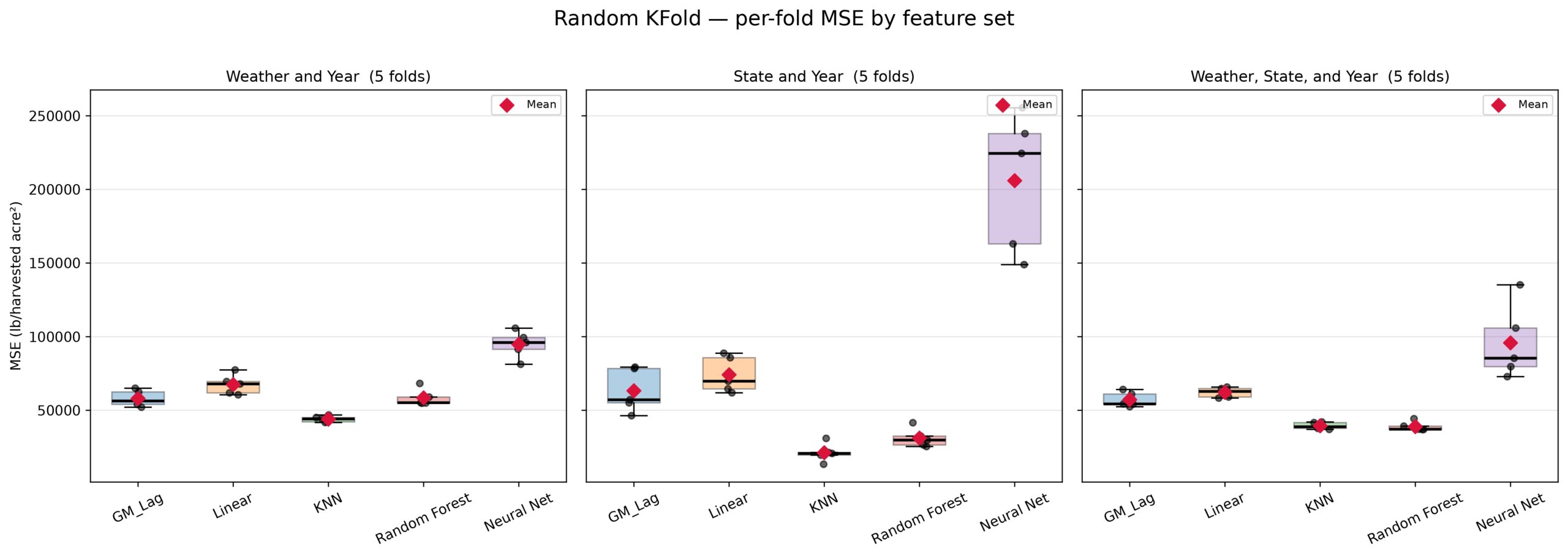
For our first approach of weather and year data with Random KFold, we found KNN to be the only statistically significant model that performed better than GM Lag. KNN had an MSE of 43,981 while GM Lag had an MSE of 57,986. Notably, GM Lag was statistically better than Linear Regression with Weather and Year only.
For our second approach of state and year data with Random KFold, we found both Random Forest and KNN Regression to be statistically significantly better than GM Lag. KNN Regression performed the best with an MSE of 21,189 and Random Forest with an MSE of 31,138 while GM Lag had an MSE of 63,262. The lowest MSE was 20,000 less than the weather only dataset, suggesting that weather parameters are noisy for KNN regression. Contrastingly, Neural Network’s MSE increased from 94,774 to 205,953 when changing to state and year features.
In our third approach of weather, state, and year data, Random Forest and KNN Regression performed better than GM Lag, with Random Forest Regression having an MSE of 38,929, KNN Regression having an MSE of 39,465, and GM Lag having an MSE of 57,228. Linear Regression was statistically worse than GM Lag with an MSE of 62,148. Finally, Neural Network’s MSE dropped back down to 95,791 which is similar to its MSE on Weather and Year data.
Across all datasets, KNN Regression outperformed GM Lag on these Random Kfolds. Additionally, GM Lag notably outperformed Linear Regression across all datasets. Lastly, using State and Year data, KNN regression achieved the lowest MSE among all approaches, while Neural Networks increased significantly using the same dataset. As seen in Figure 2, Neural Networks trained on State data had a much larger inter quartile range than other models, evident through the box length.
Time Series Results
| Time Series Results | |||||
| GM Lag | Linear Regression | KNN Regression | Random Forest | Neural Network | |
| Weather/Year MSE | 72,667 ± 15,632 | 80,893 ± 23,703 | 51,387 ± 19,617 | 71,752 ± 13,852 | 415,581 ± 88,416 |
| Weather/Year MAE | 209.7 ± 22.5 | 221.5 ± 35.7 | 173.1 ± 36.7 | 214.3 ± 23.3 | 558.2 ± 68.9 |
| Weather/Year R² | 0.309 ± 0.168 | 0.240 ± 0.205 | 0.509 ± 0.194 | 0.325 ± 0.100 | -2.871 ± 0.666 |
| State/Year MSE | 80,456 ± 12,412 | 85,738 ± 13,807 | 33,647 ± 13,922 | 55,921 ± 12,595 | 384,166 ± 82,589 |
| State/Year MAE | 220.7 ± 27.8 | 239.0 ± 25.7 | 142.3 ± 31.3 | 185.5 ± 30.4 | 543.9 ± 63.3 |
| State/Year R² | 0.236 ± 0.132 | 0.187 ± 0.138 | 0.684 ± 0.124 | 0.476 ± 0.088 | -2.581 ± 0.758 |
| Full MSE | 72,054 ± 14,193 | 75,305 ± 18,253 | 46,928 ± 17,929 | 56,507 ± 13,033 | 382,668 ± 79,801 |
| Full MAE | 211.4 ± 20.8 | 215.4 ± 28.9 | 163.5 ± 35.7 | 191.9 ± 27.0 | 537.9 ± 62.3 |
| Full R² | 0.311 ± 0.168 | 0.287 ± 0.178 | 0.554 ± 0.171 | 0.470 ± 0.095 | -2.533 ± 0.765 |
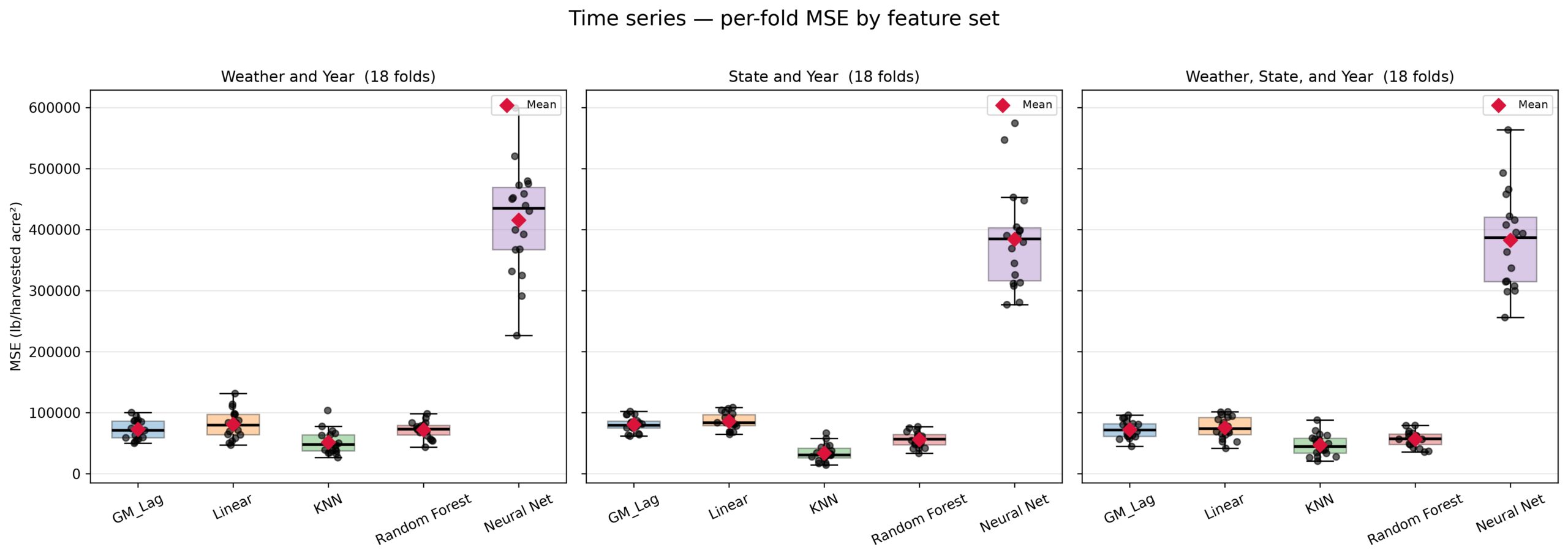
For our first approach using weather and year data, the only model that performed significantly better than GM Lag was KNN regression, with KNN Regression having an MSE of 51,387 and GM Lag having an MSE of 72,667. Additionally, GM Lag was statistically better than Linear Regression. Random Forest was statistically insignificant to GM Lag.
For our second approach using state and year data, both Random Forest and KNN Regression were significantly better than GM Lag, similar to Approach 2 Results in Random KFold (Table 1). KNN Regression had an MSE of 33,647, Random Forest had an MSE of 55,921, and GM Lag had an MSE of 80,456. Contrasting to KFold scheme results, neural network’s MSE dropped when moving to the State and Year Dataset.
Finally, with our third approach with weather, state, and year data, we found that both Random Forest and KNN Regression did the best with Random Forest and KNN Regression having a significantly better MSE than GM Lag. KNN Regression had an MSE of 46,928, Random Forest had an MSE of 56,507, and GM Lag had an MSE of 72,054. While GM Lag and Linear Regression were not statistically significant, GM Lag had a lower MSE than Linear Regression, following the direction in both Random KFold and Time Series.
Across all datasets, Neural Networks had a much larger MSE than in Random KFold with MSE ranging from 382,000 to 415,000 in the Time Series.
Group KFold
| Group KFold Results | |||||
| GM Lag | Linear Regression | KNN Regression | Random Forest | Neural Network | |
| Weather/Year MSE | 139,839 ± 93,338 | 99,608 ± 74,009 | 153,097 ± 74,182 | 102,167 ± 55,121 | 157,325 ± 139,718 |
| Weather/Year MAE | 280.7 ± 87.6 | 245.0 ± 102.8 | 312.4 ± 86.6 | 254.1 ± 87.0 | 316.6 ± 145.9 |
| Weather/Year R² | -1.129 ± 0.805 | -0.513 ± 0.800 | -2.374 ± 3.815 | -0.680 ± 0.869 | -1.993 ± 2.609 |
| State/Year MSE | 133,404 ± 89,043 | 111,476 ± 21,520 | 189,039 ± 110,106 | 112,277 ± 60,460 | 194,484 ± 96,141 |
| State/Year MAE | 280.6 ± 77.1 | 276.6 ± 40.0 | 299.0 ± 96.3 | 264.8 ± 84.5 | 394.7 ± 110.7 |
| State/Year R² | -0.974 ± 0.425 | -1.071 ± 1.012 | -1.875 ± 0.927 | -0.734 ± 0.376 | -3.450 ± 2.460 |
| Full MSE | 152,428 ± 115,238 | 114,854 ± 64,491 | 162,166 ± 70,618 | 98,298 ± 61,713 | 165,890 ± 70,458 |
| Full MAE | 294.5 ± 111.6 | 277.4 ± 81.8 | 325.3 ± 82.5 | 247.9 ± 94.6 | 342.4 ± 83.9 |
| Full R² | -1.195 ± 0.961 | -0.875 ± 0.749 | -2.609 ± 3.927 | -0.448 ± 0.439 | -2.218 ± 1.817 |
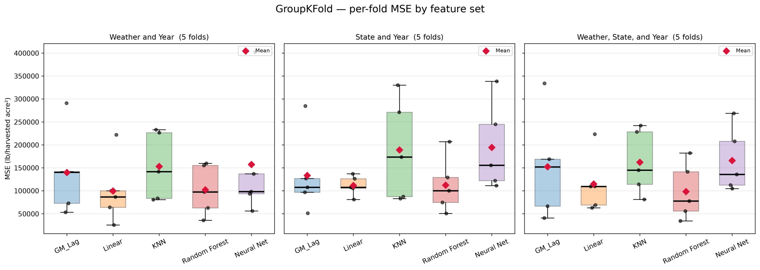
For our first approach using weather and year data, no models were statistically different than GM Lag. Despite this, the mean MSE of GM Lag throughout all datasets in Group KFold were higher than the MSE of Linear Regression.
Although a statistical comparison was not made on models between datasets, all models besides GM Lag had a lower mean MSE when using Weather and Year data as opposed to State and Year data. Furthermore, Neural Network’s MSE was the highest when using state and year data, similar to the Neural Network results in Random KFold.
For our third approach with weather, state, and year, we found that Random Forest was the only statistically better model in this whole approach with an MSE of 98,298 while GM Lag had an MSE of 152,428. However, all models in all datasets in GroupKFold had a negative R2 score.
Leave One Group Out
| Leave One Group Out Results | |||||
| GM Lag | Linear Regression | KNN Regression | Random Forest | Neural Network | |
| Weather/Year MSE | 149,991 ± 322,107 | 119,650 ± 183,094 | 128,710 ± 139,919 | 100,978 ± 108,990 | 217,419 ± 365,411 |
| Weather/Year MAE | 263.1 ± 260.2 | 251.3 ± 201.7 | 287.9 ± 178.2 | 253.6 ± 162.7 | 325.5 ± 271.1 |
| Weather/Year R² | -5.189 ± 11.069 | -6.006 ± 12.357 | -7.794 ± 14.101 | -5.190 ± 9.052 | -7.628 ± 13.106 |
| State/Year MSE | 154,631 ± 367,581 | 106,496 ± 114,651 | 190,331 ± 309,181 | 117,104 ± 132,634 | 186,260 ± 244,483 |
| State/Year MAE | 268.8 ± 265.7 | 261.0 ± 155.9 | 299.2 ± 283.5 | 264.1 ± 188.3 | 340.1 ± 241.1 |
| State/Year R² | -4.479 ± 6.910 | -4.953 ± 8.180 | -6.533 ± 10.945 | -5.210 ± 9.244 | -9.224 ± 6.569 |
| Full MSE | 165,750 ± 370,817 | 124,324 ± 191,054 | 137,584 ± 144,056 | 98,973 ± 111,588 | 626,372 ± 2,015,143 |
| Full MAE | 276.1 ± 275.2 | 263.9 ± 198.3 | 301.2 ± 182.5 | 245.9 ± 166.9 | 435.0 ± 587.2 |
| Full R² | -5.648 ± 11.427 | -6.137 ± 12.038 | -8.110 ± 13.672 | -4.790 ± 8.928 | -60.044 ± 219.088 |
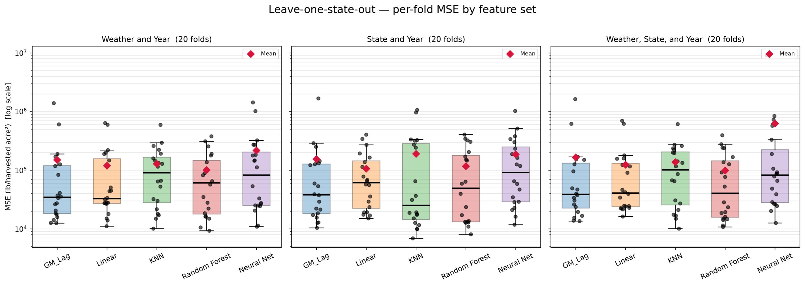
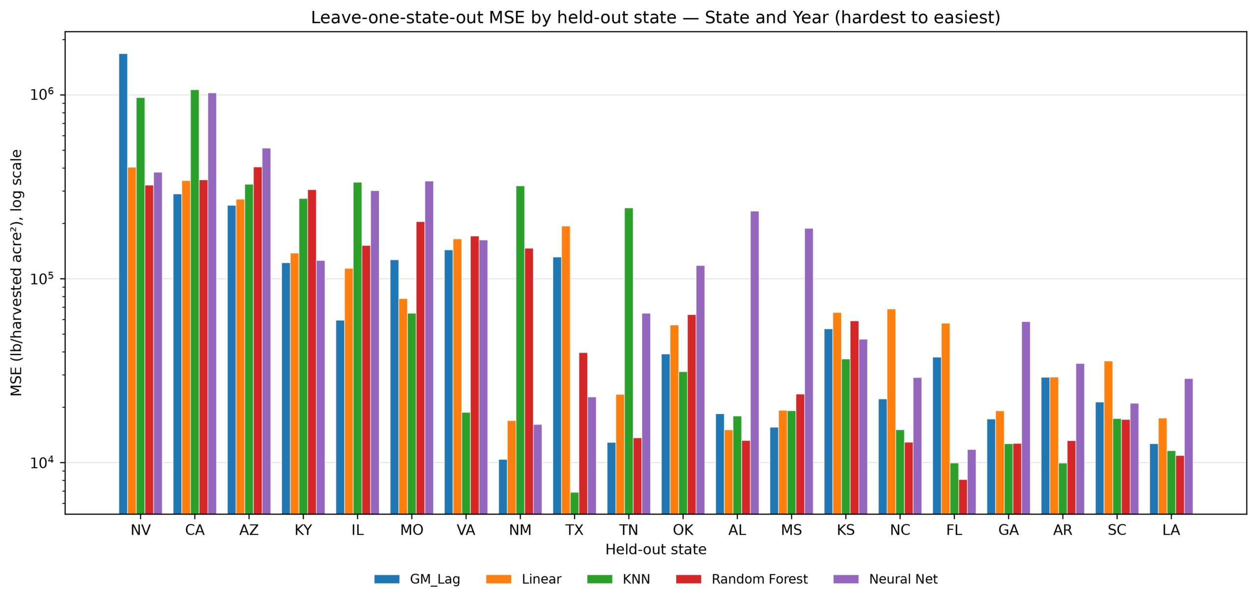
Among all datasets in Leave One State out, there were none that were statistically significant to GM Lag. Performance varied widely depending on the left out state, with all models having an MSE Standard deviation that was higher than their mean MSE. As seen in Figure 6, the states with the highest average MSE were western states such as Nevada, California, and Arizona. Furthermore, northern states such as Illinois were among the harder to predict, while Southeastern states such as Georgia and Louisiana were among the easiest to predict.
There was no clear direction in what datasets caused the lower MSE, which differed from other approaches. Neural Networks achieved its lowest MSE with State and Year data which contrasted the direction found in Random KFold and Time Series. Contrastingly, Random Forest achieved their lowest MSE using the combined dataset.
Autocorrelation Results
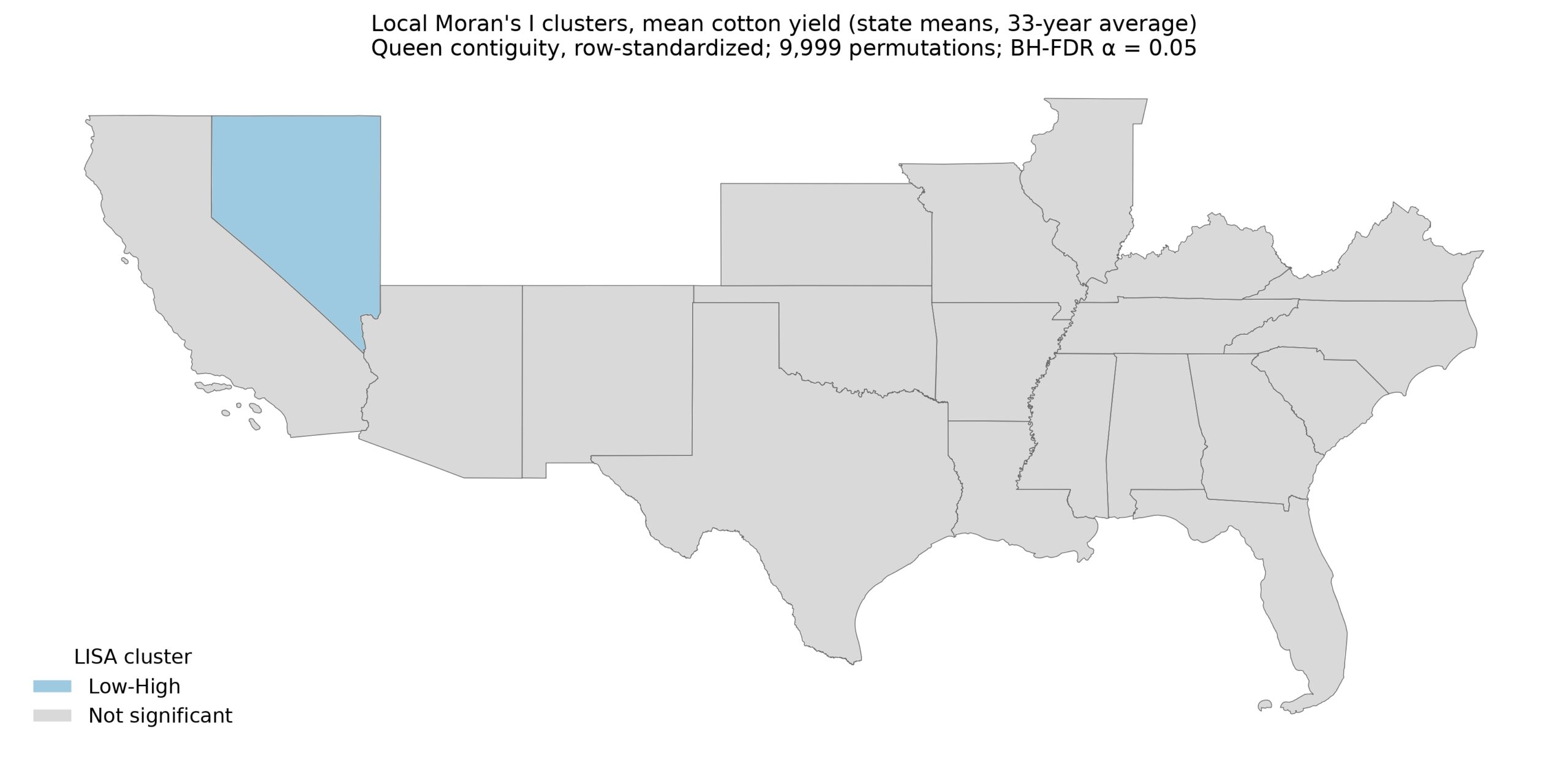
Our autocorrelation measures achieved a state averaged Global Moran’s I of +0.1097 and a pseudo p-value of 0.1443, showing a weakly positive spatial autocorrelation that is not statistically significant. We found one significant Local Moran’s I state in Nevada that had a low-high relationship (Figure 7).
Linear and Quadratic Year Testing
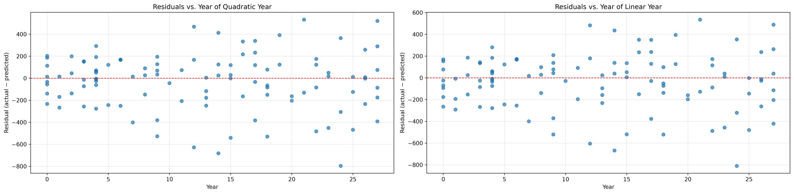
Two OLS models were fit on a full dataset with linear years and a full dataset with linear and quadratic years. The linear OLS model achieved an MSE of 65784 and an R2 score of 0.480. The quadratic OLS model achieved an MSE of 65610 with an R2 score of 0.481. We found a p-value of 0.139 from the nested F-test, showing that the differences between Linear and Quadratic years could be up to noise and insignificant. Furthermore, the recorded residual plots in Figure 8 do not show noticeable difference between Linear and Quadratic model. Furthermore, the residuals show a scattered pattern across years. Therefore, for all our models, linear years were used to not add unnecessary complexity.
Discussion
Among the 3 datasets and 4 cross validation schemes we tested, we found that GM Lag consistently achieved a lower mean MSE than a non spatial Linear Regression on KFold and Time Series across all datasets. Contrastingly, GM Lag consistently achieved a higher mean MSE than Linear Regression on Group KFold and Leave One Group Out. This pattern likely shows that GM Lag relied heavily on using past sample yield of its predicted state from its training dataset. A major issue with repurposing GM Lag for state-wide yield is that it counts its own state as a neighbor, as explained in the methodology. Therefore, Leave One Group Out and Group KFold were a better indicator of the strength of spatial relationships. Since GM Lag became reliant on using yield from its own state, when predicted state information was not available in training such as in Group KFold, performance fell. This suggests that GM Lag didn’t fully understand the coarse and weak spatial relationships that was intended because it generalized worse on unseen states than linear regression.
Despite the noticeable difference GM Lag had on Linear Regression in KFold and Time Series, the statistically insignificant Global Moran’s I of +0.10 supports that what gave GM Lag the advantage was likely not spatial patterns with neighboring states but instead information about its own state’s yield. This demonstrates that own state cotton yield is a better indicator of prediction accuracy as opposed to neighboring state’s yield. Therefore, the hypothesized benefit that spatial models would receive was not present at the state-wide level.
Since Global Moran’s I is on a scale of -1 to +1, a +0.10 Global Moran’s I value with a pseudo-p-value of 0.1443 is likely due to noise, showing that spatial patterns are likely not present at this high level. The Global Moran’s I value is considered insignificant because p>0.05. Furthermore, the corrected Local Moran’s I choropleth map having only one significant state further support that there is no spatial pattern between states (Figure 7). Therefore, its strength disproves our hypothesis that spatial relationships would give spatial models a significant edge over non-spatial models.
Neural Networks had the most consistent and highest MSE on the Time Series Cross Validation Scheme. Considering that Time Series uses a sliding window look back of 10 years and is the dataset with the lowest training size, the lowered performance is likely due to lower samples in training because of the large architecture of the model. Although increasing the epoch count would allow more time for the model to train, it would likely overfit as a result. Neural networks performed the worst in all approaches besides state and year dataset in Leave One Group Out. Considering the low dataset size and large model architecture, the model likely has too many weights for this problem.
KNN regression achieved the lowest MSE on the Random KFold scheme with only state data. Since state data is encoded with center coordinates, KNN regression likely relied on comparing past training samples for the predicted state to predict yield, suggesting that in-state cotton yield is a better indicator of yield than a neighboring state. Furthermore, this reliance is supported in schemes that included every state in the training data where KNN regression achieved a lower mean MSE than other models. It is additionally supported in schemes that didn’t include predicted state in training samples where Random Forest achieved a much lower MSE.
In KNN Regression for KFold and Time Series, weather likely cluttered KNN’s ability to find predicted state in training samples. This claim is supported when looking at KNN mean MSE in Time Series and Random KFold where it achieved the best performance when using the state and year dataset, a significantly worse performance when using combined weather, state and year dataset, and the worst performance when using weather and year dataset.
However, when KNN Regression was applied to Leave One Group Out and Group KFold, it had a much higher mean MSE than Random Forest. This suggests that KNN Regression was relying heavily on using predicted state samples from training data because it couldn’t generalize to new states, similar to GM Lag.
In cross validation schemes that required generalizing to new states, the lowest mean MSEs were in Linear Regression and Random Forest Regression. In these schemes, the lowest MSEs were never achieved using State and Year dataset. We speculate that only years and state coordinates on data models have never seen were too sparse of input features to generalize to new states. Therefore, it is possible that generalizing to new states is best predicted when weather parameters are used. However, when data about predicted states are in the training sample, weather parameters are noisy for KNN Regression.
A limitation to predicting state-wide yields using geospatial models is that it is repurposing geospatial models for a broader task that it was not designed to do. Normally, geospatial models receive a unique point for each sample and has neighbors of varying distances or large detailed neighbors. Since a state dataset was merged for each state, using a Queen matrix averages each yield of every sample of a neighboring state, demonstrating how state-wide predictions don’t provide the resolution that geospatial models were designed for. Additionally, since GM Lag was asked to find spatial patterns between centers of states as opposed to in-state or farm level patterns, spatial patterns are likely weak. The yield values are one per each state which could be affected by a number of factors, demonstrating how state spatial relationships are difficult to confirm.
Furthermore, the models are being asked to do regression on a small dataset of 528 samples while having up to 23 input features. This low sample size, broad spatial resolution, and obscure spatial set up lowers what can be claimed from this research of how models perform.
Finally, we report 95% confidence intervals for each model vs. reference comparison across all feature sets and cross validation schemes. We didn’t apply any correction for multiple testing (such as Bonferroni or FDR). Therefore, there is a high chance that a significant label could be more than 5% more likely due to chance. Therefore, the results of this study should be exploratory rather than confirmatory.
The approaches utilizing weather data are intended to be used to determine how good of a predictor weather parameters such as drought days and max temperature have on predicting cotton yield. However, the weather approaches cannot be used to predict future yields because the weather parameters collected cannot be determined until the end of the season. The only state and year approaches in Time series prediction are intended to be used for real time forecasting of cotton yield since they don’t rely on data that cannot be measured at time of planting.
Since some input features to these models may not be available at time of planting, such as average temperature or max inches of precipitation, we choose to clarify the applications of different feature sets and cross validation schemes to the real world. All of the weather parameters are unattainable at time of planting. Time series only models could be used to generalize and predict future yields and are intended for that purpose. All other models are used to interpret how significant different features or weather patterns are in predicting state wide cotton yield.
To further this research, this study only tests one spatial model, SAR that lags neighboring samples of the dependent variable. This suggests that other spatial models such as SEM that utilizes errors in neighboring states and SLX that lag independent variables in predictions could result in spatial models performing better than non spatial models in agricultural predictions. Therefore, since this research only tests one spatial model, claims that Geospatial models always perform worse than non spatial models cannot be confirmed and may not apply to other spatial models.
For next steps, test a variety of spatial models, such as ones that average independent variables or errors on similar datasets. Secondly, use a dataset with higher spatial resolution such as ones with specific farm locations and use GM Lag to predict and compare results to non-spatial models. In summary, we compared results from geospatial models to various non spatial models and found that GM Lag cannot outperform adaptable non spatial models at the state-wide level due to shared geometries for each state and little to no autocorrelation. We used a spatial approach to predict cotton yield which can be further applied to predicting other crop yields.
Supplementary Material
References
- S. Leo, M. De Antoni Migliorati, P. R. Grace. Predicting within‐field cotton yields using publicly available datasets and machine learning. Agronomy Journal. Vol. 113, pg. 1150–1163, 2021 https://doi.org/10.1002/agj2.20543 [↩] [↩]
- M. Hussain, A. F. Tariq, A. Nawaz, M. Nawaz, A. Sattar, S. Ul-Allah, A. Wakeel. Efficacy of fertilizing method for different potash sources in cotton (gossypium hirsutum l.) nutrition under arid climatic conditions. PLOS ONE. Vol. 15, pg. e0228335, 2020 https://doi.org/10.1371/journal.pone.0228335 [↩]
- J. L. Ping, C. J. Green, R. E. Zartman, K. F. Bronson. Exploring spatial dependence of cotton yield using global and local autocorrelation statistics. Field Crops Research. Vol. 89, pg. 219–236, 2004 https://doi.org/10.1016/j.fcr.2004.02.009 [↩]
- A. Mitra, S. Beegum, D. Fleisher, V. R. Reddy, W. Sun, C. Ray, D. Timlin, A. Malakar. Cotton yield prediction: a machine learning approach with field and synthetic data. IEEE Access. Vol. 12, pg. 101273–101288, 2024 https://doi.org/10.1109/ACCESS.2024.3418139 [↩]
- L. E. D. O. Aparecido, K. C. D. Meneses, G. Rolim De Souza, M. J. N. Carvalho, W. B. S. Pereira, P. A. Da Silva, T. D. S. Santos, J. R. D. S. C. De Moraes. Algorithms for forecasting cotton yield based on climatic parameters in brazil. Archives of Agronomy and Soil Science. Vol. 68, pg. 984–1001, 2022 https://doi.org/10.1080/03650340.2020.1864821 [↩] [↩]
- R. J. G. M. Florax, P. Nijkamp. Misspecification in linear spatial regression models. SSRN Electronic Journal. 2003 https://doi.org/10.2139/ssrn.459500 [↩] [↩]
- K. Kumari, S. Yadav. Linear regression analysis study. Journal of the Practice of Cardiovascular Sciences. Vol. 4, pg. 33, 2018 https://doi.org/10.4103/jpcs.jpcs_8_18 [↩] [↩]
- S. Zhang, D. Cheng, Z. Deng, M. Zong, X. Deng. A novel k nn algorithm with data-driven k parameter computation. Pattern Recognition Letters. Vol. 109, pg. 44–54, 2018 https://doi.org/10.1016/j.patrec.2017.09.036 [↩] [↩]
- J. K. Jaiswal, R. Samikannu. Application of random forest algorithm on feature subset selection and classification and regression. in 2017 World Congress on Computing and Communication Technologies (WCCCT) pg. 65–68, IEEE, Tiruchirappalli, Tamil Nadu, India, 2017 https://doi.org/10.1109/WCCCT.2016.25 [↩] [↩]
- M. Islam, G. Chen, S. Jin. An overview of neural network. American Journal of Neural Networks and Applications. Vol. 5, pg. 7, 2019 https://doi.org/10.11648/j.ajnna.20190501.12 [↩] [↩]
- P. Garg. Understanding geospatial data: in Advances in Geospatial Technologies (eds L. Gaur & P. K. Garg) pg. 1–14, IGI Global, 2023 https://doi.org/10.4018/978-1-6684-7319-1.ch001 [↩]
- A. Getis. Reflections on spatial autocorrelation. Regional Science and Urban Economics. Vol. 37, pg. 491–496, 2007 https://doi.org/10.1016/j.regsciurbeco.2007.04.005 [↩]
- W. Mu, D. Tong. Choropleth mapping with uncertainty: a maximum likelihood–based classification scheme. Annals of the American Association of Geographers. Vol. 109, pg. 1493–1510, 2019 https://doi.org/10.1080/24694452.2018.1549971 [↩]
- D. Chicco, M. J. Warrens, G. Jurman. The coefficient of determination r-squared is more informative than smape, mae, mape, mse and rmse in regression analysis evaluation. PeerJ Computer Science. Vol. 7, pg. e623, 2021 https://doi.org/10.7717/peerj-cs.623 [↩] [↩]
- R. Bivand, W. G. Müller, M. Reder. Power calculations for global and local moran’s. Computational Statistics & Data Analysis. Vol. 53, pg. 2859–2872, 2009 https://doi.org/10.1016/j.csda.2008.07.021 [↩] [↩]
- D. J. Biau, B. M. Jolles, R. Porcher. P value and the theory of hypothesis testing: an explanation for new researchers. Clinical Orthopaedics & Related Research. Vol. 468, pg. 885–892, 2010 https://doi.org/10.1007/s11999-009-1164-4 [↩] [↩]
- A. Saha. Effect of climate change on commodity yields, https://www.kaggle.com/datasets/abhisaha97/effect-of-climate-change-on-commodity-yields, 2021 [↩]
- Y. Jung. Multiple predicting k -fold cross-validation for model selection. Journal of Nonparametric Statistics. Vol. 30, pg. 197–215, 2018 https://doi.org/10.1080/10485252.2017.1404598 [↩]
- T. M. H. Hope. Linear regression. in Machine Learning pg. 67–81, Elsevier, 2020 https://doi.org/10.1016/B978-0-12-815739-8.00004-3 [↩]
- G. Guo, H. Wang, D. Bell, Y. Bi, K. Greer. KNN model-based approach in classification. in On The Move to Meaningful Internet Systems 2003: CoopIS, DOA, and ODBASE (eds R. Meersman, Z. Tari & D. C. Schmidt) Vol. 2888 pg. 986–996, Springer Berlin Heidelberg, Berlin, Heidelberg, 2003 https://doi.org/10.1007/978-3-540-39964-3_62 [↩]
- P. T. R. A comparative study on decision tree and random forest using r tool. IJARCCE. pg. 196–199, 2015 https://doi.org/10.17148/IJARCCE.2015.4142 [↩]
- M. Bataineh, T. Marler. Neural network for regression problems with reduced training sets. Neural Networks. Vol. 95, pg. 1–9, 2017 https://doi.org/10.1016/j.neunet.2017.07.018 [↩]
- A. Jadon, A. Patil, S. Jadon. A comprehensive survey of regression-based loss functions for time series forecasting. in Data Management, Analytics and Innovation (eds N. Sharma, A. C. Goje, A. Chakrabarti & A. M. Bruckstein) Vol. 998 pg. 117–147, Springer Nature Singapore, Singapore, 2024 https://doi.org/10.1007/978-981-97-3245-6_9 [↩]