Unsupervised Anomaly Detection in TESS Light Curves Using an Uncertainty-aware RNN-VAE and Consensus Ensemble of Latent-space Outlier Detectors

March 29, 2026

Abstract

Astronomical light curves provide a high-cadence record of stellar brightness variability, but the scale of modern surveys makes systematic discovery of rare behaviors difficult without automated methods. We present an unsupervised anomaly-detection pipeline for processed Transiting Exoplanet Survey Satellite (TESS) light curves that combines representation learning with complementary outlier detectors. Starting from 3,659 processed light curves produced by an MIT lab preprocessing pipeline, we apply non-imputing missing-value handling and a minimum-information filter (<20 valid paired samples) to obtain 3,593 light curves for analysis. A recurrent variational autoencoder (RNN-VAE) is trained to learn a compact latent representation; anomalies are scored using (i) VAE reconstruction error (a proxy for low reconstruction likelihood), (ii) density-based outlier structure in standardized latent space using HDBSCAN, and (iii) isolation scores in standardized latent space using Isolation Forest. We select operating points via sensitivity analyses over reconstruction thresholds (across training epochs), HDBSCAN hyperparameters, and Isolation Forest contamination, prioritizing shortlist stability under small perturbations. Under the selected settings, reconstruction scoring flags 398 objects (11.1%), HDBSCAN flags 256 (7.1%), and Isolation Forest flags 230 (6.4%). An agreement-based ensemble reduces method-specific false positives and yields 226 consensus candidates (6.29%) flagged by at least two detectors, including a strict subset of 116 objects (3.23%) flagged by all three. We provide a reproducible workflow, robustness criteria, and a manual vetting checklist to support scientific follow-up of ensemble-selected candidates.

Keywords: anomaly detection, unsupervised learning, variational autoencoder, HDBSCAN, Isolation Forest, reconstruction

Introduction

Astronomical time‑domain surveys now deliver light curves at a scale where rare and scientifically valuable behaviors can be missed by manual inspection alone. In the Transiting Exoplanet Survey Satellite (TESS) mission, instrumental systematics (e.g., sector‑dependent trends, discontinuities, and data gaps) are interleaved with astrophysical variability, complicating rule‑based screening and making labeled anomaly sets scarce¹^,²^,³^,⁴^,⁵. Unsupervised anomaly detection provides a natural alternative: instead of relying on predefined templates, models can learn the dominant structure of the data and flag observations that deviate from it

In this study we analyze 3,659 processed TESS light curves provided by a Massachusetts Institute of Technology (MIT) lab processing pipeline and apply filtering designed to avoid imputation‑driven artifacts and low‑information series, yielding a final working set of 3,593 light curves for scoring and sensitivity analysis. We develop an end‑to‑end pipeline that (i) applies per‑object robust clipping and normalization to preserve intrinsic morphology while controlling scale variation and outliers, (ii) learns a compact representation with an uncertainty‑aware recurrent variational autoencoder (RNN‑VAE), and (iii) scores anomalies using complementary detectors on both reconstruction space and latent space⁶^,⁷.

Specifically, we compute three anomaly signals: (1) VAE reconstruction‑based scores that highlight light curves the model cannot accurately reproduce (a reconstruction‑likelihood proxy for atypical structure), (2) density‑based outlier structure in standardized latent space using HDBSCAN, and (3) tree‑ensemble isolation scores in the same standardized latent space using Isolation Forest⁸^,⁹^,¹⁰. Because each detector can fail in different ways—reconstruction metrics can be sensitive to noise and calibration, while latent‑space detectors depend on the learned embedding geometry—we ensemble their outputs and prioritize consensus candidates for follow‑up.

Our results show partial overlap between detectors, consistent with their complementary inductive biases. The consensus ensemble yields 226 candidates (6.29% of the dataset) flagged by at least two methods, and a strict shortlist of 116 candidates (3.23%) flagged by all three. Beyond producing these shortlists, we contribute a sensitivity‑driven selection procedure based on threshold stability and hyperparameter robustness, and we provide a manual vetting checklist intended to support downstream inspection and scientific follow‑up of ensemble‑selected anomalies¹¹^,¹².

Data

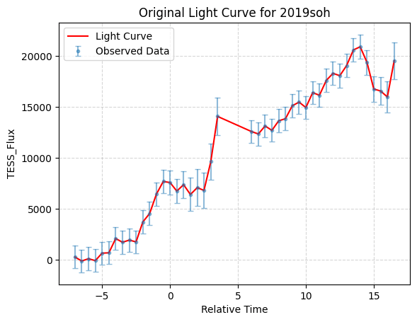
We analyze a curated dataset of processed TESS light curves provided by an MIT laboratory preprocessing pipeline. Because the files were delivered as preprocessed time-series products, mission acquisition metadata (e.g., sector identifiers and cadence) were not consistently available and are therefore not used as selection variables in this study. We treat the provided columns (relative_time, tess_flux, tess_uncert) as the primary observables and describe all additional transformations that we apply in Section Preprocessing: Per-object Robust Clipping, Normalization, and Uncertainty Weights.The dataset consists of 3,659 unlabeled CSV light-curve files, each corresponding to a single object. Each file contains time-series data with three columns: relative_time, tess_flux, and tess_uncert. Figure 1 is a randomly selected light curve file, representing the original light curve of object 2019soh, including the relative time, flux, and flux uncertainty values. To construct a unified dataset for this analysis, we combined all individual light curve files into a single dataset. To associate each data point with its corresponding object, we extracted an identifier from the file name and added it as a new column, object_name. For example, for a file named lc_2019soh_processed, the object_name was derived as 2019soh, where “lc” and “processed” are common prefixes and suffixes shared across all file names. The final dataset comprises four columns: relative_time, tess_flux, tess_uncert, and object_name.

To ensure that anomaly signals are not driven by imputation artifacts, we removed missing measurements without filling (i.e., no interpolation or forward/backward filling). After removing missing values, we excluded any light curve with fewer than 20 valid time–flux pairs since sequences below this length provide insufficient information for stable representation learning and reconstruction-error estimation. The final cleaned dataset contains 3,593 light curves (98.2% of the initial population), which we randomly partitioned at the object level into a training set and validation set using a 0.9 / 0.1 split with a fixed random seed (random state = 42). This object-level split prevents leakage of information between training and validation and provides a consistent basis for all sensitivity studies and downstream anomaly scoring.

Since light curves represent time-series data, we organized the dataset as a nested 2D array. To standardize the time values across all objects, we shifted the start time of each light curve to zero using

(1) $\begin{equation*} t' = t - \min(t) \end{equation*}$

Figure 1 | Original light curve for object 2019soh.

Methods

This section describes the data preprocessing, representation learning model, anomaly scoring methods, and ensemble decision rule used to construct a shortlist of unusual light curves⁴^,⁵.

Pipeline Overview and Design Goals

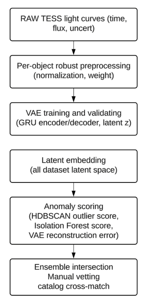
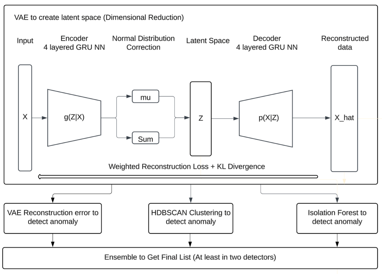
Our goal is to detect rare or unusual light curve morphologies with minimal assumptions and no labeled training set. Figure 2 summarizes the end-to-end workflow. The pipeline consists of:¹³^,¹¹

Preprocessing of each light curve with robust per-object clipping and normalization, incorporating uncertainty weights when available (see preprocessing section).
Representation learning with an uncertainty-aware RNN-VAE that generates both a reconstruction $\hat{x}$ and latent statistics $\mu, \log \sigma^2$ (see representation learning section).
Three anomaly signals:
a. Reconstruction error $e(x)$ (see reconstruction error section)
b. HDBSCAN outlier score in latent space (see HDBSCAN section)
c. Isolation Forest outliers in latent space (see Isolation Forest section)
Ensemble consensus to produce robust shortlists (see ensemble section).

Preprocessing: Per-object Robust Clipping, Normalization, and Uncertainty Weights

TESS light curves can contain outliers, discontinuities, and sector-dependent systematics. To reduce sensitivity to rare, extreme artifacts while preserving object-specific morphology, we apply per-object robust clipping using the median and a scaled median absolute deviation (MAD). We then normalize each object to reduce scale differences across stars and to allow the model to focus on shape rather than amplitude. When uncertainty estimates are available, we incorporate them as weights so that high-uncertainty points contribute less to the training objective¹⁴.

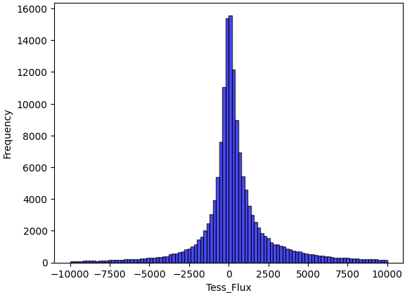
When performing the raw data distribution for all data points, the minimum tess_flux is -3.1e8, the maximum tess_flux is 1.2e7, approximately 0.1% of the tess_flux exceeded 1.1e6 or fell below -1.1e6, and approximately 7.3% of the tess_flux exceeded 1e4 or fell below -1e4. The distribution of tess_flux is illustrated in Figure 3, which shows that most of the data lies within the range of -5,000 to 5,000. The extreme data is from peak of transient light curves typically, a transient light curve example shown in Figure 5 after normalization.

Figure 3 | Distribution of raw tess_flux values across all cadences before robust clipping.

Per-object processing is central because TESS transients exhibit large between-object differences in baseline and scale. If a global normalization is applied across all measurements, embeddings may reflect brightness differences more than temporal shape. We therefore normalize each object independently using robust statistics.

Robust clipping. For each object, we compute the median flux m and the median absolute deviation (MAD). We then cap only extreme flux values outside $m \pm k \cdot \mathrm{MAD}$ at the boundary. In this study, we use $k=25$ , chosen via a sensitivity sweep to balance artifact suppression against preservation of astrophysical morphology.

(2) $\begin{equation*} f_{\text{clipped}}(t) = \operatorname{clip}\big(f(t),\, m - k\cdot \mathrm{MAD},\, m + k\cdot \mathrm{MAD}\big) \end{equation*}$

Per-object normalization. After clipping, we compute robust_median and robust_mad per object and normalize:

(3) $\begin{equation*} f_{\text{norm}}(t) =\frac{f_{\text{clipped}}(t) - \mathrm{robust\_median}} {\mathrm{robust\_mad}} \end{equation*}$

Uncertainty scaling and weights. Uncertainties are scaled by the same robust_mad. We compute inverse-variance weights $\omega (t)=\frac{1}{\sigma\_{\mathrm{norm}}(t)^2+\epsilon}$ and (optionally) normalize weights within each object so $\max (\omega)=1$ to stabilize training.

(4) $\begin{equation*} \text{uncert}_{\text{scaled}}(t) = \frac{\text{tess\_uncert}(t)}{\mathrm{robust\_mad}}\end{equation*}$

(5) $\begin{equation*} w_{\text{raw}}(t) = \frac{1}{\text{uncert}_{\text{scaled}}(t)^2 + \varepsilon}, \qquad \varepsilon = 10^{-10} \end{equation*}$

(6) $\begin{equation*} \text{weights}_{\text{normalized}}(t) = \frac{w_{\text{raw}}(t)}{\max\!\left(w_{\text{raw}}(t)\right)} \end{equation*}$

Sensitivity Studies for Preprocessing Choices

We justify preprocessing parameters using two complementary sensitivity analyses:¹⁴

(A) Robust clipping factor k: evaluate $k \in {3,5,10,15,25}$ and track

(i) fraction of points clipped,
(ii) morphology preservation (peak amplitude and turning points).

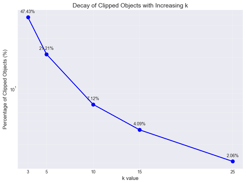
To determine the optimal k value for the robust normalization procedure, we conducted a sensitivity analysis by evaluating multiple k values, and the clipped point percentage result is shown in Figure 4. The choice of k represents a critical balance between removing spurious outliers and preserving genuine astrophysical signals in transient light curves.

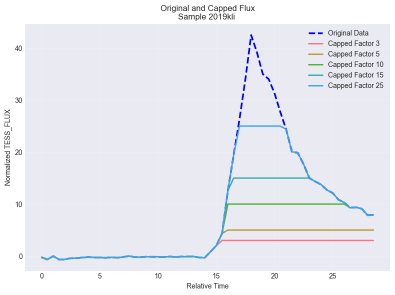
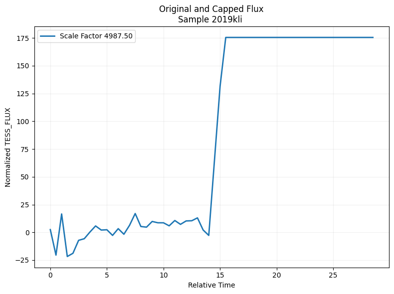
Figure 5a shows the normalized flux profiles with unclipped and clipped by various k, whose object name is 2019kli with the maximum tess_flux of 1.2e7. It can be observed that the maximum tess_flux is over 40 times as MAD for this object. Figure 5b shows the percentage of objects clipped with k. When $k=25$ , only 2.1% of the total 3,593 objects were impacted by the capping process.

Figure 5a | Example normalized light curve (object 2019kli) under different MAD factors k.

Figure 5b | Fraction of objects affected by clipping as a function of MAD factor k.

(B) Per-object vs global normalization: we did a comparison study by normalizing the flux globally, which means all flux is divided by a common scale factor, which is the minimum of absolute 5 or 95 percentiles. The normalized result for the same object 2019kli was shown in Figure 7. It can be observed that the light curve pattern was completely altered, as compared to the same object shown in Figure 5a using robust MAD normalization and clipping.

Figure 6 | Example normalization using a global scale factor (shown for comparison).

Evaluation Metrics and Robustness Criteria

Because ground-truth anomaly labels are not available, we evaluate robustness using internal consistency metrics and stability under parameter perturbation:⁴

Anomaly fraction: proportion of objects flagged as anomalous.
Shortlist stability: Jaccard similarity between anomaly sets produced under adjacent parameter choices (e.g., neighboring hyperparameter values).
Noise fraction (HDBSCAN): fraction of points labeled as noise.
Cluster persistence and membership probability (HDBSCAN): diagnostic measures of cluster stability and assignment confidence.
Sensitivity regimes (Isolation Forest): analysis of how the anomaly signal changes as contamination varies, separating stable from overly sensitive settings.

These metrics guide parameter selection toward stable, reproducible behavior rather than arbitrary anomaly rates.

Representation Learning with an Uncertainty-aware RNN-VAE

Variational Autoencoders (VAEs) are generative models that encode complex data into a lower-dimensional latent space while preserving a probabilistic interpretation. Introduced by Kingma and Welling in 2013⁶, VAEs combine neural networks with variational inference to learn both a reconstruction model and a structured latent distribution, making them well suited for representation learning in unlabeled time-series data¹⁵^,⁷.

VAEs are built on the concept of an autoencoder, which consists of two neural networks: an encoder and a decoder. The encoder compresses input data into a latent representation, and the decoder reconstructs the original data from this compressed latent space. Unlike traditional autoencoders, VAEs incorporate probabilistic modeling, which provides two main advantages: they can generate new samples from the learned distribution, and they provide a meaningful latent space that captures the underlying structure of the data.

The VAE in this study uses a Gated Recurrent Unit (GRU) encoder–decoder. GRUs are recurrent neural networks designed to mitigate vanishing-gradient issues and model temporal dependencies efficiently, which is appropriate for variable-length TESS light-curve sequences¹⁶. Related recurrent architectures such as LSTMs have also been applied to time-series anomaly detection¹⁷.

Each light curve is a variable-length sequence $x(t) = [t, f_{\mathrm{norm}}(t)]$ . The encoder outputs $\mu(x)$ and $\log \sigma^2(x)$ ; a latent sample $z$ is obtained via the reparameterization trick and decoded to reconstruct $\hat{x}(t)$ . The loss function is a weighted Evidence Lower Bound (ELBO), which consists of two components:

Reconstruction Loss: Computed as the mean squared error (MSE) between the original input and the reconstructed output, this ensures that the reconstruction of the data is accurate enough for analysis. Here we use weighted MSE to incorporate flux uncertainty.
Kullback-Leibler Divergence (KLD): This term regularizes the model by approximating a Gaussian distribution in the latent space. It provides a continuous latent representation and prevents overfitting.

The total ELBO loss is represented as:

(7) $\begin{equation*} ELBO=\omega(t)\cdot MSE+KLD \end{equation*}$

The architecture of VAE and subsequent anomaly detection is shown in Figure 8.

Figure 7 | Pipeline overview: preprocessing → uncertainty-aware RNN-VAE → anomaly signals (reconstruction error, HDBSCAN, Isolation Forest) → consensus ensemble.

VAE Setup and Convergence Monitoring

We use a recurrent encoder–decoder architecture with a hidden size of 128, latent size of 16, and 4 recurrent layers. We train with Adam (learning rate 10-4) for up to 1400 epochs, saving checkpoints periodically. Convergence is monitored using validation reconstruction error and ELBO components (reconstruction and KLD).¹⁸

The basic parameters used in the VAE are listed as follows:

Input size = 2
Hidden size = 128
Latent size = 16
Output size = 1
Number of GRU layers (encoder and decoder) = 4
Optimizer = Adam
Learning rate = 1.e-4
Drop out = 0.2
Epochs = 1400

As stated in the previous section, we use a 90/10 train–validation split (random_state = 42) and monitor ELBO components (reconstruction loss and KLD) to verify stable convergence before downstream scoring.

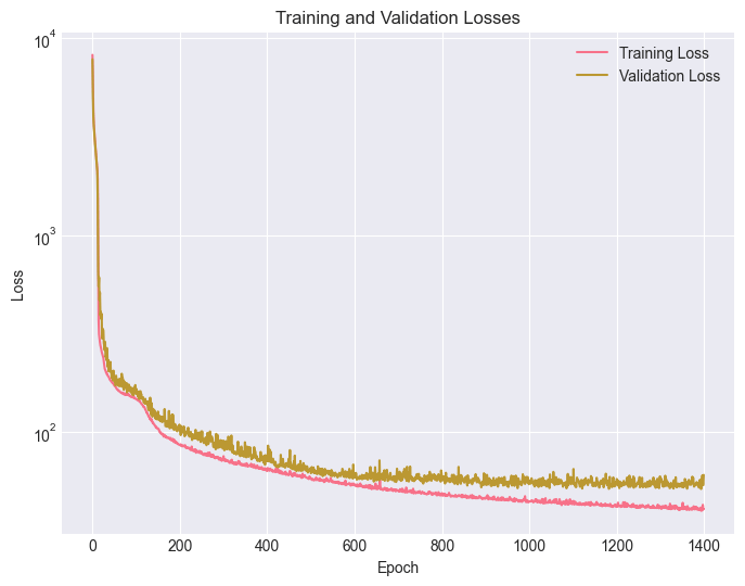
Early stopping was used for a case study, with patience parameter as of 2 which means checking validation loss increasing for the last 2 epochs) and the training process was not triggered by early stopping until it is completed at 800 epochs. The training and validation loss behavior had the same pattern as in Figure 10a which did not use early stopping.

VAE Reconstruction-error Anomaly Detection

Reconstruction error is the (weighted) mean squared error over normalized flux values across all timesteps in an object. Reconstruction error is used as an anomaly score: objects in the high-error tail are candidates⁶.

Sensitivity study (epoch $\times$ threshold)

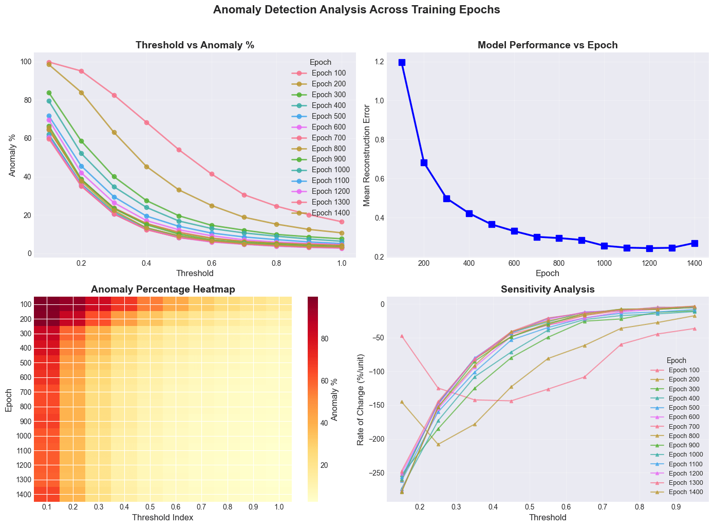
To select a defensible checkpoint and threshold, we perform a two-dimensional sweep: epochs from 200 to 1400 (step 100) and reconstruction-error thresholds from 0.2 to 0.9 (step 0.1). For each epoch, t, we compute the anomaly fraction:

(8) $\begin{equation*} p(\tau;epoch)=\frac{1}{N}\sum_{i=1}^N I[e_i(epoch)\geq \tau] \end{equation*}$

where $I[\cdot]$ is the indicator function, when the condition is met, then 1, else 0.

Results are summarized in Figure 9 and Table 1. The validation reconstruction curve flattens around 700 epochs, indicating convergence, and threshold–anomaly curves stabilize thereafter. We therefore select the converged checkpoint (epoch $\approx$ 700) and choose $\tau = 0.5$ , which corresponds to 398 anomalies (11.0%).

Figure 8 | VAE Reconstruction Error Sensitivity Study.

Epoch	0.2	0.3	0.4	0.5	0.6	0.7	0.9	Mean Error
200	84.00%	63.00%	45.40%	33.20%	25.00%	18.80%	12.60%	0.6815
400	51.90%	35.00%	23.90%	16.80%	12.90%	10.50%	7.50%	0.4216
500	45.30%	29.60%	19.50%	14.10%	10.80%	8.50%	5.90%	0.3643
600	41.90%	26.50%	17.20%	12.50%	9.20%	7.10%	5.00%	0.3309
700	38.40%	23.60%	15.60%	11.00%	8.10%	6.20%	4.80%	0.301
800	38.30%	23.50%	15.40%	10.70%	7.80%	6.30%	4.60%	0.2948
900	38.70%	23.60%	14.90%	10.10%	7.00%	5.70%	4.00%	0.2856
1000	36.30%	21.50%	13.40%	9.20%	6.50%	5.20%	3.70%	0.2562
1100	35.40%	20.60%	12.70%	8.30%	6.20%	4.90%	3.30%	0.2463
1200	35.40%	20.50%	12.30%	8.10%	6.00%	4.80%	3.10%	0.2436

Table 1 | Summary: Anomaly Percentages by Epoch and Threshold

HDBSCAN Anomaly Detection

Hierarchical Density-Based Spatial Clustering of Applications with Noise (HDBSCAN) is an advanced clustering algorithm that identifies clusters based on density variations in the data. Unlike traditional density-based clustering methods such as DBSCAN, HDBSCAN builds a hierarchical tree of clusters and condenses it to select the most stable structures. This capability makes HDBSCAN particularly effective for datasets with variable densities, such as light curves derived from astronomical observations⁹,¹⁹.

The latent space features generated by the VAE were input into the HDBSCAN algorithm for clustering analysis. HDBSCAN identifies dense clusters representing typical behaviors in the dataset and labels sparse regions as noise or anomalies. Points classified as noise or outliers by HDBSCAN are flagged as potential anomalies, which may correspond to astrophysical phenomena or instrumental irregularities.

HDBSCAN and related density-based methods have seen growing use in astronomy for exploratory clustering and anomaly discovery in high-dimensional representations (e.g., within the Astronomaly framework and related work combining clustering with anomaly scoring). Related unsupervised approaches have been applied to transient discovery in survey light curves²⁰.

We apply HDBSCAN to the latent mean vectors $\mu_i$ (standardized per dimension) to identify low-density outliers. HDBSCAN yields $(i)$ cluster labels, $(ii)$ membership probabilities, and $(iii)$ outlier scores (higher indicates more outlier-like). We define anomalies by thresholding the outlier score.

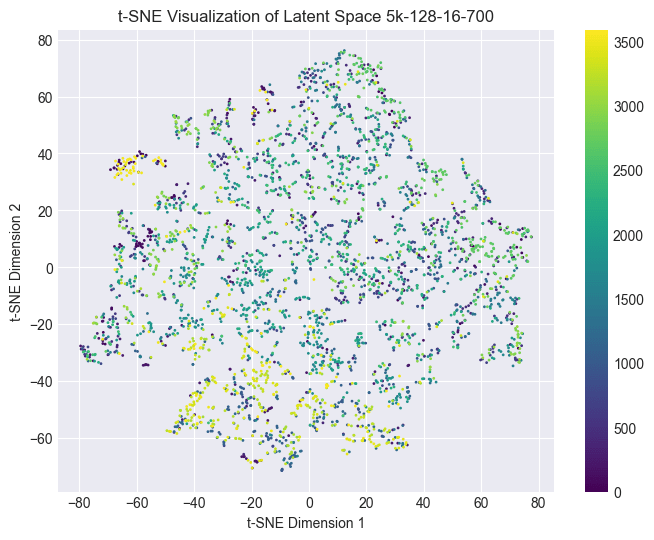
For qualitative visualization only, we include a 2-D t-SNE embedding of the standardized latent vectors in the Supplement; all clustering and anomaly scoring are performed in the full latent space.

Sensitivity study (mcs $\times$ ms $\times$ threshold)

We sweep min_cluster_size and min_samples over a grid and evaluate multiple outlier-score thresholds, prioritizing shortlist stability and diagnostic quality. We compute anomaly shortlist stability using Jaccard similarity of anomaly sets across adjacent settings, and we track noise fraction, mean membership probability, and cluster persistence. Based on stability and diagnostic criteria, we select min_cluster_size $=$ 15, min_samples $=$ 8, and an outlier-score threshold of $0.6$ . This yields 256 anomalies (7.125%) and strong shortlist stability as shown in Table 2. (mcs: min_cluster_size, ms: min_samples, jac: Jaccard similarity score)

Additional HDBSCAN parameters (defaults unless stated): metric=euclidean, cluster_selection_method=eom.

mcs	ms	rank_score	anomaly_frac	persist_mean	Prob_clustred	jac_ms	jac_mcs
15	8	0.72	7.13	0.19	0.73	0.88	0.78
15	10	0.69	7.85	0.19	0.70	0.88	0.57
10	8	0.69	3.90	0.17	0.80	0.84	0.78
5	8	0.65	3.90	0.17	0.80	0.68	0.78
10	12	0.65	3.48	0.17	0.82	0.84	0.59
10	10	0.64	3.67	0.17	0.81	0.84	0.57
5	12	0.60	1.53	0.15	0.89	0.68	0.59
5	10	0.59	1.56	0.14	0.89	0.68	0.57

Table 2 | Sensitivity study of HDBSCAN

Isolation Forest Anomaly Detection

Isolation Forest (IF) is an unsupervised algorithm for anomaly detection that isolates rare points using random partitioning: anomalies tend to be separated with fewer splits than typical points¹⁰.

We apply Isolation Forest to the standardized latent vectors $\mu$ . IF isolates anomalies via random partitions, assigning lower decision-function scores to more anomalous points. IF requires specifying contamination c, the expected outlier fraction.

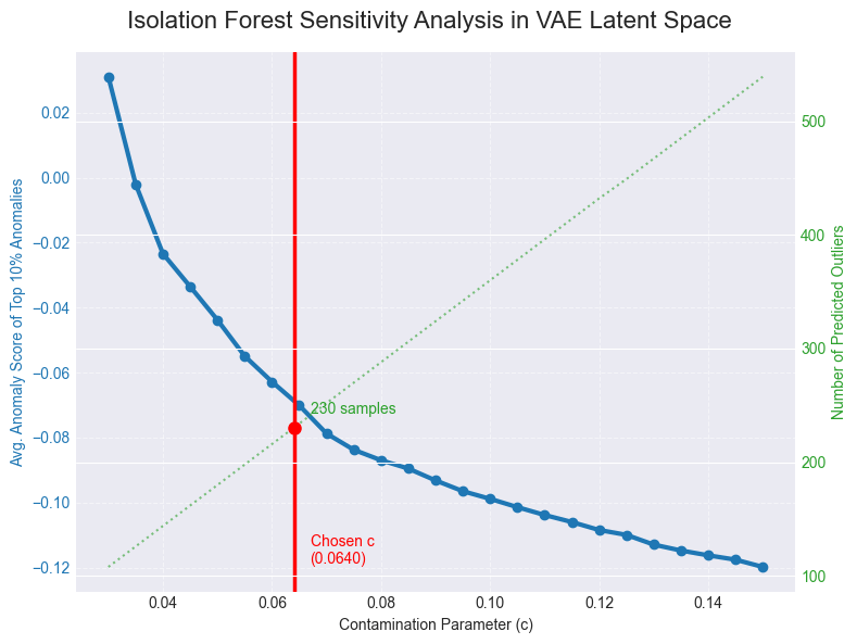
Score distribution and contamination sensitivity

We first inspect the distribution of IF decision scores (Figure 9) to confirm a concentrated bulk with a tail of low scores. We then perform a sensitivity sweep over contamination $c$ , tracking $(i)$ a signal-stability metric based on the mean score of a fixed extreme subset (top $K$ %) and $(ii)$ the expected linear increase in predicted outlier count with c. The sensitivity curve exhibits a transition from a highly sensitive regime at small c to a flatter regime where increases in c primarily add borderline points. We select c=0.064 near the onset of the stable regime, yielding approximately 230 outliers (6.4%).

Isolation Forest parameters (defaults unless stated): $n \_ estimators=1000, random \_ state=42$ .

Figure 9 | Isolation Forest sensitivity analysis in VAE latent space; selected contamination c = 0.064 (red).

Ensemble Intersection and Manual Vetting

Each detector flags anomalies under a different definition. To improve robustness and reduce detector-specific false positives, we combine detector outputs using an agreement-based ensemble. We assign each object a consensus score equal to the number of detectors that flag it (0–3). We report two shortlists:¹¹^,¹³

Moderate consensus ( $\geq$ 2): increases recall while suppressing single-detector artifacts.
Strict consensus (3-of-3): a high-confidence shortlist robust across all detectors.

Manual vetting is applied as a final qualitative check to confirm that shortlisted objects exhibit non-trivial astrophysical structure rather than trivial preprocessing failures. For each candidate we $(i)$ verify that the time–flux series contains $\geq 20$ valid cadences after cleaning, $(ii)$ check for step-like discontinuities consistent with scattered-light or stitching artifacts, $(iii)$ confirm that anomalies persist under small changes to preprocessing hyperparameters within the stable regime, and $(iv)$ visually inspect the normalized light curve for coherent variability (e.g., transit-like dips, flare-like spikes, or structured trends) before prioritizing follow-up.

Implementation Details and Reproducibility

All experiments were implemented in Python using PyTorch for the RNN-VAE²¹^, scikit-learn for Isolation Forest and supporting utilities ²², and the hdbscan package for density-based clustering⁹. We fix random seeds where applicable (including $random \_ state =42$ for the object-level $0.9/0.1$ train–validation split in Section Data to ensure repeatability of sensitivity sweeps and shortlist comparisons²³^,²²^,²⁴.

Key model hyperparameters are listed in Section VAE setup and Convergence Monitoring (latent dimension 16; GRU hidden size 128; 4-layer encoder/decoder; dropout 0.2; Adam optimizer with learning rate $1\times 10^{-4}; 1400$ epochs with checkpointing). All latent-space detectors operate on standardized latent mean vectors (zero mean, unit variance per dimension) to place distances and axis-wise densities on a comparable scale before clustering or isolation-based scoring.

Results

We report convergence diagnostics for the representation learner and summarize the anomaly candidates identified by each detector, followed by the intersection-based ensemble shortlist¹³^,¹¹.

Model convergence and reconstruction behavior

Training of the RNN-VAE showed rapid improvement in reconstruction quality during early epochs, followed by a clear plateau, indicating convergence of the learned representation. The average validation loss (weighted $MSE + KLD$ ) decreased steeply up to mid-training and then flattened, with diminishing improvements beyond approximately 700 epochs, as shown in Figure 10a. This convergence pattern is consistent with the threshold–anomaly curves across epochs (Figure 9): at early epochs, small changes in the reconstruction-error threshold produce large swings in anomaly percentage, whereas after convergence, the anomaly-rate curves become substantially more stable. Based on this stabilization, we selected the checkpoint at epoch 700 for downstream anomaly scoring and detector ensemble⁶^,¹⁸.

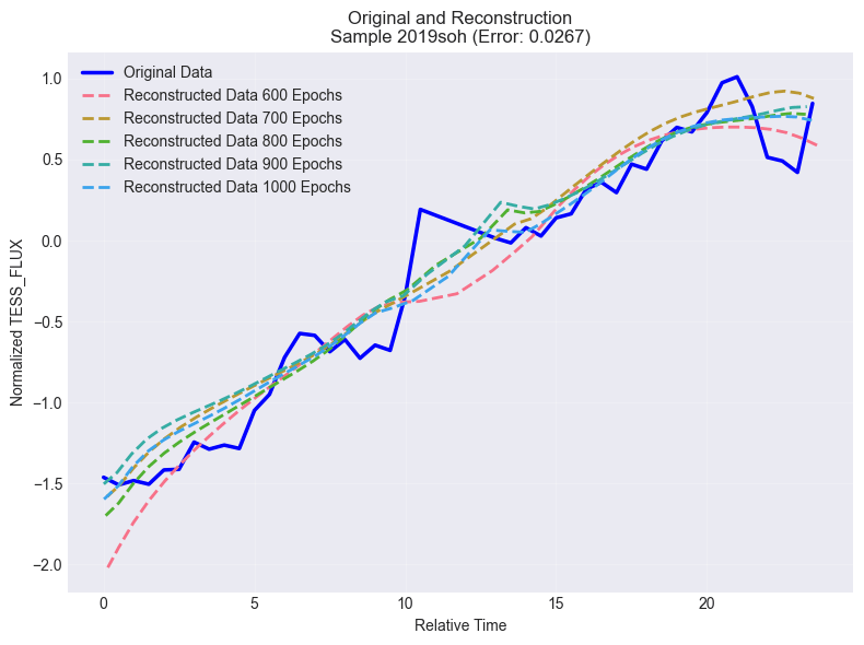
Figure 10b shows the normalized light curve for object 2019soh mentioned earlier, before and after training. The reconstruction curves caught the pattern of the original curve, and the model performed well for the studied epochs.

Figure 10a | Training loss vs. epochs for the VAE model.

Figure 10b | Normalized light curves before and after training for object 2019soh.

Reconstruction-error anomalies

At epoch $\sim 700$ , the reconstruction-error threshold selects 398/3593 objects ( $\sim 11.1$ %) as anomalous with a threshold of 0.5. The threshold–anomaly curve exhibits a knee near this operating point, whereas lower thresholds increasingly include borderline cases⁶.

HDBSCAN latent-space anomalies

Using the selected HDBSCAN hyperparameters and outlier-score threshold 0.6, HDBSCAN identifies 256/3593 ( $\sim7.1$ %) anomalies. The chosen setting lies in a stable regime of the sweep with high anomaly-set stability and low noise fraction⁹.

Isolation Forest latent-space anomalies

Isolation Forest with the selected contamination identifies approximately 230/3593 ( $\sim 6.4$ %) outliers. Score-distribution inspection and contamination sensitivity indicate a stable region before overly permissive settings begin to add borderline points¹⁰.

Ensemble shortlist results

The three detectors partially overlap, reflecting complementary definitions of “unusual.” Pairwise overlaps are 38 (HDBSCAN∩IF only), 63 (HDBSCAN∩Reconstruction only), and 9 (IF∩Reconstruction only). In total, 226 objects are flagged by at least 2-of-3 detectors, and 116 objects are flagged by all 3 detectors, forming a high-confidence shortlist for prioritized follow-up¹¹.

Counts and fractions of light-curve objects flagged as anomalous under a three-detector ensemble consisting of VAE reconstruction-error thresholding, HDBSCAN latent-space outlier scoring, and Isolation Forest latent-space isolation. Pairwise overlaps are decomposed into “exactly two” agreements by subtracting the three-way intersection. We report both a moderate-consensus shortlist ( $\geq 2$ agreement) and a strict shortlist (3-of-3 agreement), which prioritize robustness to method-specific false positives.

Combination (flagged by…)	Count	% of dataset
HDBSCAN $\cap$ Isolation Forest ∩ Reconstruction (3-of-3)	116	3.23%
HDBSCAN $\cap$ Isolation Forest only (exactly 2-of-3)	38	1.06%
HDBSCAN $\cap$ Reconstruction only (exactly 2-of-3)	63	1.75%
Isolation Forest $\cap$ Reconstruction only (exactly 2-of-3)	9	0.25%
At least 2-of-3 (ensemble shortlist)	226	6.29%
All 3-of-3 (strict shortlist)	116	3.23%

Table 3 | Detector agreement structure and ensemble shortlist sizes.

Discussion

We interpret the detector behaviors, discuss why consensus improves reliability in unlabeled settings, and outline practical validation steps and limitations for TESS survey light curves⁴^,¹³.

Why ensembling improves reliability in unsupervised settings

Unsupervised anomaly detection in survey data is vulnerable to detector-specific false positives. Reconstruction error may be inflated by noise bursts or detrending artifacts; density-based methods can be affected by local neighborhood structure; and Isolation Forest can isolate sparse points even when they are not scientifically interesting. An agreement-based ensemble reduces these risks by prioritizing candidates that remain anomalous across independent criteria. In this pipeline, consensus anomalies represent objects that are simultaneously difficult to reconstruct and isolated in latent structure, improving robustness for downstream vetting⁴.

Interpreting the anomaly fractions

The anomaly fractions differ across detectors because they measure different properties and are calibrated differently. The reconstruction-error detector is intentionally broader (11.0%) to capture time-domain deviations, while latent-space detectors are slightly more conservative ( $\sim$ 6–7%) to focus on structural outliers in representation space. These rates are best interpreted as screening yields rather than estimates of true astrophysical anomaly prevalence. The ensemble step provides a principled way to reconcile differing detector yields into a stable shortlist¹³.

Convergence and threshold stability as justification

The reconstruction-error sensitivity analysis provides two layers of justification: (i) the model converges around 700 epochs, and (ii) post-convergence anomaly fractions are stable under epoch changes for mid-range thresholds. Similarly, HDBSCAN and IF parameter selection is anchored to stability criteria rather than matching a desired anomaly fraction. This emphasis on stability reduces the risk that conclusions depend on fragile hyperparameter choices⁶.

Latent-space quality and collapse considerations

A common VAE risk is posterior collapse, where latent variables carry little information and anomalies become harder to separate in representation space. Mixed per-dimension variability (some latent dimensions near unit-scale and others smaller) suggests partial under-utilization but not full collapse. Importantly, the observed stability of HDBSCAN anomaly sets across sweeps indicates that latent structure is sufficiently informative for outlier detection under the chosen settings. Future work can quantify latent utilization more directly using KL-per-dimension diagnostics or mutual information estimates⁶.

TESS catalogue cross-validation

To contextualize the ensemble candidates, we cross-matched all 3,593 objects and each shortlist against public TESS catalog classification fields (public catalogs link: https://tess.mit.edu/public/tesstransients/lc_bulk/count_transients.txt). Across the full dataset, 479/3,593 objects (13.3%) are catalog-classified (i.e., not labeled “Unclassified”). Within the $\geq$ 2-of-3 consensus shortlist (N=226), 28 objects (12.4%) are catalog-classified, and within the strict 3-of-3 shortlist (N=116), 12 objects (10.3%) are catalog-classified. The majority of ensemble-selected candidates therefore lack an existing catalog classification (198/226 and 104/116, respectively), suggesting that the consensus rule preferentially surfaces under-characterized light-curve morphologies; however, uncataloged objects can include both genuinely rare astrophysical variability and residual instrumental/systematic effects. For follow-up, we recommend screening candidates using pipeline data-quality and contamination indicators²⁵^,³.

It is important to note that the training population used in this study is a subset of objects with available processed light curves and therefore does not represent the full population of sources present in the public TESS catalogues. Consequently, “anomalous” scores are defined relative to this limited reference set: objects that are well characterized (i.e., catalog-classified) may still appear unusual with respect to the subset’s dominant morphology distribution and instrument/noise properties. In that sense, catalog-classified objects flagged as anomalies may reflect genuine rarity within the analyzed population rather than errors in the catalogue. A key next step is to expand the training and scoring population to include a substantially larger (ideally complete) set of TESS light curves processed under consistent criteria. With a broader reference distribution, the learned embedding and detector decision boundaries should better reflect the true survey population and may reduce the incidence of catalog-classified objects being selected as anomalies.

Limitations and future validation

The primary limitation is the absence of ground-truth labels, which prevents direct precision/recall evaluation. Future validation will use injection-and-recovery tests (synthetic transits/flares and controlled artifacts) and systematic crossmatching to quantify detection performance. Additionally, manual vetting can introduce subjective bias; future work will define stricter, reproducible inspection criteria and expand review to larger samples⁵^,¹³. Recent work on training anomaly detectors under label noise and contamination includes latent outlier exposure, which could be adapted to light-curve representations²⁶.

Conclusions

We developed an unsupervised anomaly detection pipeline for TESS light curves that integrates reconstruction error from an uncertainty-aware RNN-VAE with two complementary latent-space detectors (HDBSCAN and Isolation Forest). We selected detector operating points using sensitivity analyses and stability-based criteria, yielding screening sets of 398 (11.0%) reconstruction-error candidates, 256 (7.125%) HDBSCAN candidates, and $\sim$ 230 (6.4%) Isolation Forest candidates on objects. We then combined these signals via an agreement-based ensemble, producing both a broad $\geq$ 2-of-3 shortlist and a strict 3-of-3 shortlist for high-confidence anomalies. This approach demonstrates that stability-driven calibration and consensus ensembling can generate defensible anomaly shortlists in large photometric surveys without labeled data, forming a foundation for catalog cross-matching and targeted scientific follow-up.

Appendix A. t-SNE latent-space visualization

t‑SNE is used only as a qualitative visualization of the standardized 16‑D latent means. Unless otherwise stated, we use $perplexity =30$ , $learning \_ rate =200$ , $n \_ iter = 1000$ , $init = 'pca'$ , and $random \_ state = 42$ ; we verified that the global structure is similar under ±10 changes in perplexity and alternate random seeds (visual check only).²⁷,²⁸.

We include a t-SNE projection of the VAE latent mean vectors as a qualitative visualization of global structure in representation space; all anomaly scoring is performed in the full latent space. Replace the placeholder below with a plot generated from the epoch $\sim$ 700 embeddings (e.g., color by detector flags or ensemble membership).

Figure A1 | Placeholder for t-SNE embedding of VAE latent mean vectors. Perplexity=30, learning rate=200, iterations=1000, random_state=42

Appendix B. Detected anomalies in the studied TESS Dataset

Detected by 3 detectors

2018eny, 2018eph, 2018fdx, 2018fhw, 2018fwm, 2018fxj, 2018glq, 2018gsg, 2018gum, 2018hql, 2018jjd, 2018jkg, 2018jms, 2018kao, 2018kjp, 2019agu, 2019ajf, 2019alv, 2019bgp, 2019cqi, 2019dtv, 2019erz, 2019esl, 2019gn, 2019hlb, 2019iiv, 2019kli, 2019nfv, 2019nng, 2019obp, 2019pco, 2019rj, 2019rvh, 2019saz, 2019sld, 2019sse, 2019tjl, 2019tlu, 2019tsu, 2019vzy, 2020aayk, 2020abbx, 2020acpv, 2020afq, 2020bxc, 2020ddi, 2020ftl, 2020fyf, 2020hgp, 2020mic, 2020rhn, 2020rkb, 2020rld, 2020rme, 2020tir, 2020tld, 2020uic, 2020wnf, 2020xgz, 2021aalc, 2021acet, 2021afte, 2021afth, 2021ageo, 2021agoa, 2021bll, 2021bma, 2021buu, 2021cmf, 2021cxp, 2021dvt, 2021efq, 2021hpf, 2021jbh, 2021ksl, 2021odw, 2021qpb, 2021qut, 2021soz, 2021wue, 2021xeq, 2021xet, 2021xgv, 2021xgy, 2021xhf, 2021xhm, 2021xhq, 2021xkr, 2021xmj, 2021xob, 2021xqg, 2021xrc, 2021xrd, 2021xuk, 2021xzu, 2021ybe, 2021yga, 2021ygg, 2021yib, 2021yjr, 2021yln, 2021ylu, 2021yps, 2021ysk, 2021yuh, 2021yyu, 2021yzg, 2021zct, 2021zdo, 2021zeu, 2021zf, 2022chy, 2022cmr, 2022dsv, 2022duk, 2022ejx

Detected by 2 or 3 detectors

2018eny, 2018eph, 2018fdw, 2018fdx, 2018fhw, 2018fwm, 2018fxj, 2018glq, 2018gsg, 2018gum, 2018gxi, 2018hib, 2018hka, 2018hkx, 2018hps, 2018hql, 2018izr, 2018jjd, 2018jkg, 2018jms, 2018kao, 2018kjp, 2019agu, 2019ahk, 2019ajf, 2019alv, 2019ayy, 2019bcp, 2019bgp, 2019caa, 2019cmb, 2019cqi, 2019dfr, 2019dtv, 2019erz, 2019esl, 2019fir, 2019gn, 2019hlb, 2019hnp, 2019iiv, 2019kag, 2019kli, 2019lru, 2019mqc, 2019nfv, 2019nng, 2019nvm, 2019obp, 2019osx, 2019pco, 2019pzj, 2019qck, 2019qoj, 2019rj, 2019rvh, 2019saz, 2019sho, 2019sld, 2019src, 2019sse, 2019sts, 2019tjl, 2019tlu, 2019tng, 2019tsu, 2019tsz, 2019ufy, 2019umq, 2019vzy, 2019xe, 2019zdo, 2019zej, 2020aayk, 2020abbx, 2020acpv, 2020adgm, 2020adsx, 2020afq, 2020bol, 2020bsb, 2020bvg, 2020bxc, 2020ddi, 2020dsl, 2020ftl, 2020fyf, 2020hgp, 2020iwn, 2020kav, 2020kur, 2020lkf, 2020mic, 2020npl, 2020nrl, 2020nyb, 2020qit, 2020rhn, 2020rkb, 2020rld, 2020rme, 2020rxw, 2020tir, 2020tld, 2020uic, 2020ut, 2020uvg, 2020vku, 2020wnf, 2020wvh, 2020xgu, 2020xgz, 2020xjp, 2020xoy, 2020zo, 2020zui, 2021aalc, 2021aanc, 2021aarc, 2021aaxr, 2021aazx, 2021abfd, 2021acet, 2021afte, 2021afth, 2021afvw, 2021ageo, 2021agoa, 2021bll, 2021bma, 2021buu, 2021ckj, 2021cmf, 2021cxp, 2021dvt, 2021efq, 2021flg, 2021gfy, 2021hit, 2021hpf, 2021jbh, 2021kei, 2021koi, 2021ksl, 2021odw, 2021oim, 2021qpb, 2021qut, 2021soz, 2021tod, 2021ttz, 2021wue, 2021wzp, 2021xeq, 2021xet, 2021xgv, 2021xgy, 2021xhb, 2021xhf, 2021xhm, 2021xhq, 2021xiw, 2021xjq, 2021xkr, 2021xku, 2021xmj, 2021xnb, 2021xni, 2021xns, 2021xob, 2021xpe, 2021xph, 2021xpn, 2021xqg, 2021xrc, 2021xrd, 2021xuk, 2021xvu, 2021xxt, 2021xzu, 2021ybe, 2021ybj, 2021yga, 2021ygg, 2021yhc, 2021yib, 2021yic, 2021yiq, 2021yjr, 2021yln, 2021ylu, 2021ynq, 2021yps, 2021ysk, 2021yuh, 2021yvo, 2021yvr, 2021yxf, 2021yyu, 2021yzg, 2021zba, 2021zbt, 2021zct, 2021zdo, 2021zeu, 2021zf, 2022amx, 2022ark, 2022cdv, 2022chy, 2022cmr, 2022djv, 2022dsv, 2022dtj, 2022dto, 2022dtp, 2022duk, 2022duz, 2022ejx, 2022ely, 2022emm, 2022exc, 2022eyw, 2022gaz, 2022kh, 2022oz

Unclassified objects after cross checking with public TESS catalogue (by 3 detectors, 104/116)

2018eny, 2018fwm, 2018fxj, 2018glq, 2018gsg, 2018gum, 2018hql, 2018jkg, 2018jms, 2018kao, 2018kjp, 2019agu, 2019ajf, 2019alv, 2019bgp, 2019cqi, 2019dtv, 2019erz, 2019esl, 2019gn, 2019hlb, 2019kli, 2019nfv, 2019nng, 2019obp, 2019pco, 2019rj, 2019rvh, 2019sld, 2019sse, 2019tjl, 2019tsu, 2019vzy, 2020aayk, 2020abbx, 2020acpv, 2020bxc, 2020ddi, 2020fyf, 2020hgp, 2020mic, 2020rhn, 2020rkb, 2020rld, 2020rme, 2020tir, 2020uic, 2020wnf, 2020xgz, 2021aalc, 2021acet, 2021afte, 2021afth, 2021ageo, 2021agoa, 2021bll, 2021buu, 2021cmf, 2021cxp, 2021dvt, 2021efq, 2021hpf, 2021jbh, 2021ksl, 2021odw, 2021qpb, 2021qut, 2021soz, 2021wue, 2021xeq, 2021xet, 2021xgv, 2021xgy, 2021xhf, 2021xhm, 2021xhq, 2021xkr, 2021xmj, 2021xob, 2021xqg, 2021xrc, 2021xrd, 2021xuk, 2021xzu, 2021ybe, 2021yga, 2021ygg, 2021yib, 2021yjr, 2021yln, 2021ylu, 2021yps, 2021ysk, 2021yuh, 2021yzg, 2021zct, 2021zdo, 2021zeu, 2021zf, 2022chy, 2022cmr, 2022dsv, 2022duk, 2022ejx

Unclassified objects after cross checking with public TESS catalogue (by 2 or 3 detectors, 198/226)

2018eny, 2018fdw, 2018glq, 2018gsg, 2018fxj, 2018fwm, 2018gum, 2018hql, 2018hps, 2018izr, 2018jms, 2018jkg, 2018kjp, 2019gn, 2019rj, 2018kao, 2019agu, 2019ajf, 2019alv, 2019xe, 2019ahk, 2019ayy, 2019caa, 2019bgp, 2019cqi, 2019cmb, 2019dfr, 2019dtv, 2019erz, 2019esl, 2019fir, 2019hnp, 2019hlb, 2019kag, 2019kli, 2019mqc, 2019nfv, 2019pco, 2019qck, 2019lru, 2019nng, 2019osx, 2019pzj, 2019qoj, 2019rvh, 2019obp, 2019tjl, 2019sld, 2019tng, 2019tsu, 2019tsz, 2019sse, 2019sts, 2019sho, 2019src, 2019umq, 2019vzy, 2019ufy, 2019zej, 2019zdo, 2020zo, 2020bsb, 2020bxc, 2020bvg, 2020ddi, 2020dsl, 2020fyf, 2020hgp, 2020iwn, 2020kav, 2020kur, 2020mic, 2020lkf, 2020nrl, 2020rld, 2020qit, 2020rxw, 2020rhn, 2020wnf, 2020rkb, 2020uic, 2020rme, 2020vku, 2020wvh, 2020tir, 2020zui, 2020xgu, 2020xgz, 2020xoy, 2020xjp, 2020aayk, 2020abbx, 2020acpv, 2020adgm, 2021zf, 2020adsx, 2021bll, 2021buu, 2021cxp, 2021dvt, 2021efq, 2021gfy, 2021cmf, 2021hit, 2021hpf, 2021flg, 2021koi, 2021ksl, 2021jbh, 2021kei, 2021oim, 2021qpb, 2021qut, 2021odw, 2021tod, 2021soz, 2021ttz, 2021xku, 2021xns, 2021xob, 2021xuk, 2021xeq, 2021yiq, 2021zbt, 2021xet, 2021xgv, 2021xgy, 2021xhb, 2021xiw, 2021zba, 2021wzp, 2021xnb, 2021yvo, 2021yvr, 2021xhf, 2021xhm, 2021xxt, 2021yga, 2021yib, 2021yic, 2021ysk, 2021aarc, 2021xjq, 2021xrc, 2021xrd, 2021ynq, 2021xni, 2021yhc, 2021yxf, 2021yzg, 2021ybe, 2021aalc, 2021abfd, 2021zct, 2021zdo, 2021aaxr, 2021afvw, 2021afte, 2021afth, 2021ageo, 2021acet, 2021agoa, 2022ark, 2022oz, 2022kh, 2022cmr, 2022amx, 2022dto, 2022chy, 2022cdv, 2022djv, 2022dtj, 2022duk, 2022gaz, 2022ely, 2022duz, 2022ejx, 2022dsv, 2022dtp

Acknowledgments

I would like to thank Cari Cesarotti for her help and support throughout the process and Tyler Moulton for useful conversations.

References

G.R. Ricker, J.N. Winn, R. Vanderspek, D.W. Latham, G.A. Bakos, J.L. Bean, Z.K. Berta-Thompson, T.M. Brown, L. Buchhave, N.R. Butler, R.P. Butler, W.J. Chaplin, D. Charbonneau, J. Christensen-Dalsgaard, M. Clampin, D. Deming, J. Doty, N. Lee, C. Dressing, E.W. Dunham, M. Endl, F. Fressin, J. Ge, T. Henning, M.J. Holman, A.W. Howard, S. Ida, J. Jenkins, G. Jernigan, J.A. Johnson, L. Kaltenegger, N. Kawai, H. Kjeldsen, G. Laughlin, A.M. Levine, D. Lin, J.J. Lissauer, P. MacQueen, G. Marcy, P.R. McCullough, T.D. Morton, N. Narita, M. Paegert, E. Palle, F. Pepe, J. Pepper, A. Quirrenbach, S.A. Rinehart, D. Sasselov, B. Sato, S. Seager, A. Sozzetti, K.G. Stassun, P. Sullivan, A. Szentgyorgyi, G. Torres, S. Udry, J. Villasenor. Transiting Exoplanet Survey Satellite (TESS). Journal of Astronomical Telescopes, Instruments, and Systems, 1(1), 014003, 2015. [↩]
J.M. Jenkins, J.D. Twicken, S. McCauliff, J. Campbell, D. Sanderfer, D. Lung, M. Mansouri-Samani, F. Girouard, P. Tenenbaum, T. Klaus, J.C. Smith, D.A. Caldwell, A.D. Chacon, C. Henze, C. Heiges. The TESS science processing operations center. In Proceedings of SPIE, 9913, 99133E, 2016. [↩]
J.D. Twicken, D.A. Caldwell, J.M. Jenkins, P. Tenenbaum, J.C. Smith, B. Wohler, M. Rose, E.B. Ting, R. Vanderspek, E. Morgan, A. Rudat, M. Fausnaugh, S. Fleming, E. Quintana. TESS Science Data Products Description Document (EXP-TESS-ARC-ICD-TM-0014, Rev F). NASA/MAST technical documentation, 2020. [↩] [↩]
V. Chandola, A. Banerjee, V. Kumar. Anomaly detection: A survey. ACM Computing Surveys, 41(3), 15, 2009. [↩] [↩] [↩] [↩] [↩]
R. Chalapathy, S. Chawla. Deep learning for anomaly detection: A survey. arXiv:1901.03407, 2019. [↩] [↩] [↩]
D.P. Kingma, M. Welling. Auto-encoding variational Bayes. arXiv:1312.6114, 2013. [↩] [↩] [↩] [↩] [↩] [↩] [↩]
J. Chung, K. Kastner, L. Dinh, K. Goel, A. Courville, Y. Bengio. A recurrent latent variable model for sequential data. arXiv:1506.02216, 2015. [↩] [↩]
J. An, S. Cho. Variational autoencoder based anomaly detection using reconstruction probability. Technical report (SNUDM-TR-2015-03), SNU Data Mining Center, 2015. [↩]
L. McInnes, J. Healy, S. Astels. hdbscan: Hierarchical density based clustering. Journal of Open Source Software, 2(11), 205, 2017. [↩] [↩] [↩] [↩]
F.T. Liu, K.M. Ting, Z.H. Zhou. Isolation forest. In 2008 IEEE International Conference on Data Mining, 413–422, 2008. [↩] [↩] [↩]
M. Lochner, B.A. Bassett. Astronomaly: Personalized interactive visual anomaly detection in astronomical data. Astronomy and Computing, 36, 100481, 2021. [↩] [↩] [↩] [↩] [↩]
M. Lochner, B.A. Bassett. A Hitchhiker’s Guide to Anomaly Detection with Astronomaly. arXiv:2201.10189, 2022. [↩]
S. Fotopoulou. A review of unsupervised learning in astronomy. Astronomy and Computing, 47, 100851, 2024. [↩] [↩] [↩] [↩] [↩] [↩]
F.R. Hampel. The influence curve and its role in robust estimation. Journal of the American Statistical Association, 69(346), 383–393, 1974. [↩] [↩]
D.J. Rezende, S. Mohamed, D. Wierstra. Stochastic Backpropagation and Approximate Inference in Deep Generative Models. In Proceedings of the 31st International Conference on Machine Learning (ICML), 1278–1286, 2014. [↩]
K. Cho, B. van Merriënboer, C. Gulcehre, D. Bahdanau, F. Bougares, H. Schwenk, Y. Bengio. Learning phrase representations using RNN encoder–decoder for statistical machine translation. In Proceedings of EMNLP 2014, 1724–1734, 2014. [↩]
P. Malhotra, L. Vig, G. Shroff, P. Agarwal. Long short term memory networks for anomaly detection in time series. In European Symposium on Artificial Neural Networks (ESANN), 2015. [↩]
D.P. Kingma, J. Ba. Adam: A method for stochastic optimization. arXiv:1412.6980, 2015. [↩] [↩]
R.J.G.B. Campello, D. Moulavi, J. Sander. Density-based clustering based on hierarchical density estimates. In Advances in Knowledge Discovery and Data Mining (PAKDD 2013), 160–172, 2013. [↩]
S. Webb, M. Lochner, D. Muthukrishna, J. Cooke, C. Flynn, A. Mahabal, S. Goode, I. Andreoni, T. Pritchard, T.M.C. Abbott. Unsupervised machine learning for transient discovery in deeper, wider, faster light curves. Monthly Notices of the Royal Astronomical Society, 498(3), 3077–3094, 2020. [↩]
A. Paszke, S. Gross, F. Massa, A. Lerer, J. Bradbury, G. Chanan, T. Killeen, Z. Lin, N. Gimelshein, L. Antiga, A. Desmaison, A. Köpf, E. Yang, Z. DeVito, M. Raison, A. Tejani, S. Chilamkurthy, B. Steiner, L. Fang, J. Bai, S. Chintala. PyTorch: An imperative style, high-performance deep learning library. In Advances in Neural Information Processing Systems (NeurIPS), 2019. [↩]
F. Pedregosa, G. Varoquaux, A. Gramfort, V. Michel, B. Thirion, O. Grisel, M. Blondel, P. Prettenhofer, R. Weiss, V. Dubourg, J. VanderPlas, A. Passos, D. Cournapeau, M. Brucher, M. Perrot, É. Duchesnay. Scikit-learn: Machine learning in Python. Journal of Machine Learning Research, 12, 2825–2830, 2011. [↩] [↩]
A. Paszke, S. Gross, F. Massa, A. Lerer, J. Bradbury, G. Chanan, T. Killeen, Z. Lin, N. Gimelshein, L. Antiga, A. Desmaison, A. Köpf, E. Yang, Z. DeVito, M. Raison, A. Tejani, S. Chilamkurthy, B. Steiner, L. Fang, J. Bai, S. Chintala. PyTorch: An imperative style, high-performance deep learning library. In Advances in Neural Information Processing Systems (NeurIPS), 2019. [↩]
Lightkurve Collaboration, J.V.D.M. Cardoso, C. Hedges, M. Gully-Santiago, N. Saunders, A.M. Cody, T. Barclay, A. Hall, T. Sagear, J. Turtelboom, W. Zhang, A. Tzanidakis, K.J. Mighell, J. Coughlin, E. Bell, Z.K. Berta-Thompson, P.K.G. Williams, A. Dotson, G. Barentsen. Lightkurve: Kepler and TESS time series analysis in Python. Astrophysics Source Code Library, ascl:1812.013, 2018. [↩]
D.A. Caldwell, P. Tenenbaum, J.D. Twicken, J.M. Jenkins, E. Ting, J.C. Smith, C. Hedges, M.M. Fausnaugh, M. Rose, C. Burke. TESS Science Processing Operations Center: full-frame image target sample. Research Notes of the AAS, 4, 201, 2020. [↩]
C. Qiu, A. Li, M. Kloft, M. Rudolph, S. Mandt. Latent outlier exposure for anomaly detection with contaminated data. In International Conference on Machine Learning (ICML), 18153–18167, 2022. [↩]
L. van der Maaten, G. Hinton. Visualizing data using t-SNE. Journal of Machine Learning Research, 9, 2579–2605, 2008. [↩]
L. van der Maaten. Accelerating t-SNE using tree-based algorithms. Journal of Machine Learning Research, 15, 3221–3245, 2014. [↩]