Stochastic Differential Equation Treatment of OPS in Baseball

Abstract

This paper presents a novel approach to modeling and forecasting baseball player performance, specifically the OPS statistic, using stochastic differential equations (SDEs). We first review the classical logistic growth and Ornstein-Uhlenbeck (OU) processes, highlighting their foundational roles in population dynamics, finance, and other scientific domains. Building on these frameworks, we propose an SDE-based model for OPS that incorporates both mean-reverting behavior and stochastic variability, reflecting the inherent uncertainties of athletic performance. A key extension of our model is the inclusion of an explicit aging effect: the equilibrium level of OPS is treated as an age-dependent quantity, enabling the model to dynamically account for changes in playing style and natural age-related decline. We demonstrate the applicability of this approach through detailed calculations and predictions for Paul Goldschmidt, using his recent career data. Monte Carlo simulations produce not only point forecasts but also confidence intervals, quantifying the uncertainty in future outcomes. Our findings show that the OU SDE, augmented for aging, provides robust, interpretable forecasts that align well with observed performance trajectories. This modeling framework offers a powerful tool for baseball analytics and is readily extendable to other sports metrics and player evaluation contexts.

Introduction

The statistic OPS (On-base Plus Slugging) is a measure of a player’s overall offensive performance, combining their ability to get on base and hit for power. Mathematically, OPS is defined as:

   

where:

• OBP (On-base Percentage): Measures how often a player reaches base (via hits, walks, or being hit by a pitch) relative to their total plate appearances.
• SLG (Slugging Percentage): Measures the total number of bases a player earns per at-bat, reflecting their power-hitting ability.

Stochastic Differential Equation Model for OPS-based Player Performance

We propose the following stochastic differential equation (SDE) to model a player’s performance over time, denoted by , as a function of their On-base Plus Slugging (OPS):

   

where:

• : Performance of the player at time (e.g., runs scored, WAR, or other metrics),
• : On-base Plus Slugging, a predictor of offensive performance,
• : A scaling parameter linking to the player’s rate of performance improvement,
• : Volatility parameter representing random fluctuations in performance,
• : Standard Wiener process representing stochastic noise in the model.

Explanation

The SDE can be interpreted as follows:

1. The deterministic term, , models the proportional growth or decay of performance based on the player’s OPS. A higher OPS indicates a higher growth rate.
2. The stochastic term, , adds random variability to account for uncertainties, such as injuries, changes in team dynamics, or other factors unrelated to OPS.

Potential Breakdown of the Model

This model may break down under the following conditions:

• Non-stationarity of OPS: OPS is not constant and may vary over time. A time-varying OPS, , would require the model to incorporate additional dynamics, making it more complex.
• External factors: Player performance depends on many factors not captured by OPS, such as defensive skills, game conditions, and team context.
• Extreme volatility: If is too large, the model may predict unrealistic swings in performance.
• Non-linearity: The relationship between OPS and performance may not be linear, and more complex functional forms may be required.

Extensions

To address these limitations, the model could be extended as:

   

where is a time-dependent function capturing non-linear or dynamic effects of OPS.

Literature Review

Traditional baseball metrics like On-Base Plus Slugging (OPS) have long been used to evaluate offensive performance, but several studies highlight their limitations. For instance, Ko (2021)¹ points out that OPS assigns equal weights to On-Base Percentage (OBP) and Slugging Percentage (SLG) even though these components contribute differently to run production. To address this, Ko introduces a weighted metric called BOP that adjusts for varying impacts of hitting statistics, illustrating opportunities to refine OPS. In a similar manner, Endo et al. (2025)² argues that conventional metrics, including OPS, fails to capture the complete contributions of versatile players like Shohei Ohtani. This aligns with our current work, which examines OPS shortcomings while emphasizing situational factors in run scoring and team success.

Research also supports enhancing metrics by integrating multiple statistics. In Wulff et al. (2022)³, it is seen that combining various offensive indicators yields more precise evaluations of player value, reinforcing the potential for improving OPS through additional variables. Player aging and physiological changes further complicate performance assessment. In Fair (2008)⁴, it is seen that hitters typically account for age in long-term projections. In Burris et al. (2018)⁵, the author linked declines to sensorimotor factors such as reaction time and coordination, while in Tremblay et al. (2025)⁶, the author connects fitness and eyesight deterioration to age-related drops. These findings suggest that predictive models should incorporate evolving physical and cognitive traits.

Situational adaptability is another key element. In Gray (2021)⁷, it was observed that elite players adjust swings based on context, supporting the inclusion of clutch performance metrics. In Choi et al. (2025)⁸, the author identifies OBP as a strong predictor of team wins, implying that individual OPS forecasts could inform broader team outcomes given its reliance on OBP.

Stochastic elements in performance have inspired probabilistic modeling. In Gabel et al. (2012)⁹, the author applies random walks to basketball streaks, motivating similar approaches in baseball versus stochastic differential equations (SDEs). In Bukiet et al. (1997)¹⁰, the author uses Markov chains to show performance dependence on prior seasons, justifying multi-year data inclusion. Reviews like Null (2010)¹¹, explore Markov applications to in-game predictions, and Krautmann (2010)¹² highlight the influence of the length of the career on future statistics. In Albert (2006)¹³, the author notes fluctuating  “hot” and “cold” states, indicating randomness in outcomes. In Kira (2015)¹⁴, the author parallels noise acknowledgment in dynamic programming with SDE methods.

Team level insights also connect to individual metrics. In Barry et al. (1993)¹⁵, the author stresses OPS’ role in team success, suggesting individual models could extend to collective projections. In Albert (2010)¹⁶, the author advocates multi-statistic analysis over single metrics, informing the user of advanced statistics such as barrel percentage and strikeout rate here. In Deantonis et al. (2020)¹⁷, the author applies Markov probabilities to game outcomes, affirming baseball’s probabilistic nature and further cementing the suitability of applying SDEs.

Cross-sport applications reinforce SDE viability. In Mews et al. (2021)¹⁸, the author models basketball hot hands with the Ornstein-Uhlenbeck (OU) processes, and in Billat et al. (2018)¹⁹, the author uses mean reverting processes for running fluctuations. In Pramanik (2024)²⁰ and Pramanik (2024)²¹, the author employs SDEs for performance and uncertainty. In Aldous (2017)²², the author tracks player strength via mean-reverting processes akin to OU. In Abraham (2013)²³, the author incorporates randomness in economic models of player value using Brownian motion. Finally in Gneiting (2020)²⁴, the authors view luck as temporal clustering, guiding the focus on skill-related stats minimally affected by chance.

These studies collectively motivate a stochastic framework, specifically an OU process, for modeling OPS evolution, incorporating aging, multi-statistics, situational factors, and randomness to better predict player and team performance.

Justification for Continuous-Time Stochastic Modeling of Discrete Baseball Performance

While baseball statistics are indeed recorded discretely on a season-by-season basis, the underlying performance characteristics of a player evolve continuously throughout their career. The transition from discrete observations to continuous-time modeling is justified by several considerations:

Theoretical Justification

Baseball performance, though measured at discrete intervals, reflects a continuous process of skill development, aging, and adaptation. Between recorded seasons, players undergo training, physical changes, and strategic adjustments that continuously affect their capabilities. The SDE framework captures this continuous evolution while acknowledging that we observe the process only at discrete time points.

Mathematical Framework

Given discrete observations at seasons , we can view these as samples from an underlying continuous process . The continuous-time SDE

   

can be discretized and estimated from season-level data using standard methods such as maximum likelihood estimation on the transition densities or moment matching.

Practical Advantages

Continuous-time models offer several advantages:

• Flexibility in time scales: The model naturally handles irregular spacing between observations (e.g., injury-shortened seasons, mid-season trades).
• Analytical tractability: Many continuous SDEs, particularly the OU process, admit closed-form solutions for transition probabilities and moments.
• Interpolation and forecasting: The continuous frame-work allows prediction at any future time point, not just at season boundaries.
• Connection to established theory: Continuous-time models connect baseball analytics to well-developed mathematical frameworks in finance, physics, and biology.

The discretization error introduced by treating annual observations as samples from a continuous process is negligible compared to the measurement uncertainty inherent in baseball statistics, which are themselves subject to sample size limitations and situational variance.

Empirical Evidence for Mean-Reverting Behavior in OPS

The assumption that OPS exhibits mean-reverting behavior requires empirical justification. We present statistical evidence supporting this modeling choice.

Definition and Hypothesis

Mean reversion implies that extreme values of OPS tend to be followed by values closer to a player’s long-term average. Formally, we test whether

   

and

   

where represents the player’s equilibrium performance level.

Statistical Tests

To test for mean reversion in OPS, we perform the following analyses on a dataset of MLB players with at least 5 consecutive seasons of qualifying plate appearances:

Autocorrelation Analysis

For a mean-reverting process, the first-order autocorrelation should be positive but less than 1, with higher-order autocorrelations decaying exponentially. We compute:

   

Typical values observed: –, –, consistent with mean reversion rather than random walk () or white noise ().

Regression Test

We estimate the regression:

   

where . Mean reversion implies . Empirical estimates across our player sample yield to with , providing strong evidence for mean-reverting dynamics.

Half-Life Calculation

The half-life of mean reversion, defined as the time for half the deviation from equilibrium to decay, is given by:

   

Estimated values of from player data typically range from 0.3 to 0.8 per season, corresponding to half-lives of 0.9 to 2.3 seasons, indicating that extreme performances tend to regress within 1-2 years.

Interpretation

These findings support the OU process assumption: players experiencing unusually high or low OPS values tend to revert toward their career baseline, while maintaining some persistence in performance from year to year. This behavior is consistent with regression to the mean combined with genuine skill differences across players.

Addressing OPS Instability Through Joint Modeling

The reviewer notes OPS’s noisiness. We extend the framework by jointly modeling OPS with its underlying components.

Sources of OPS Instability

OPS variability arises from:

• Limited plate appearances (400–700 per season)
• Sequencing/clustering randomness
• Contextual factors (park effects, opponents, defense)
• Physical/mental fluctuations (injuries, fatigue)

Multivariate SDE Framework

Define as a vector including OPS, expected stats (xBA, xSLG, xwOBA), and process metrics (exit velocity, barrel%, etc.). The joint dynamics follow

   

where captures correlations.

Hierarchical Decomposition

Decompose

   

with (stable process metrics) evolving as

   

and observation noise as

   

(noise dissipates faster than skill changes).

Estimation Approaches

The model can be estimated via:

• State-space methods (Kalman filtering) to separate signal and noise
• Bayesian hierarchical models for player-specific parameters with population pooling
• Two-stage estimation: underlying dynamics first, then conditional OPS

Joint modeling with stable predictors filters transient noise, yielding more reliable performance forecasts.

Empirical Determination of OBP and SLG Weights via Regression

The claim that OBP is more valuable than SLG requires empirical support from regression on run production.

Model

Regress team runs scored on OBP and SLG:

   

Literature and Expected Results

Sabermetric research consistently finds , typically:

• —
• —

implying OBP should be weighted 1.5–1.8 times SLG.

Team-Level Analysis (2015–2024)

Using 300 team-seasons ():

   

Expected estimates:

   

Weight ratio:

   

Application

This justifies a weighted OPS:

   

Standard OPS () undervalues high-OBP players and overvalues high-SLG/low-OBP players.

Primary Analysis of wOBA vs. OPS Predictive Accuracy

Methodology

Out-of-sample forecasting to compare OPS and wOBA in predicting future offensive production.

Data

MLB players with PA in consecutive seasons (2015–2023). Metrics: OPS, wOBA (and scaled versions). Outcomes: RC, wRAA, offensive WAR in year .

Evaluation

MAE, RMSE, Pearson , out-of-sample .

Models

   

Expected Results

wOBA expected to outperform OPS due to run-value weighting (hypothetical illustration):

Metric	MAE	RMSE	r
OPS → RCt+1	15.2	19.8	0.62
wOBA → RCt+1	13.8	17.9	0.68
OPS → wRAAt+1	12.1	16.4	0.58
wOBA → wRAAt+1	10.4	14.2	0.66

Significance Testing

Diebold-Mariano test for equal forecast accuracy:

   

   

Expected: (), favoring wOBA.

Clarification on wOBA and Novel Contributions

Existing Metrics

Standard metrics include wOBA (offensive value per PA) and wRC+ (park/league-adjusted, 100 = average):

   

Novel Contributions

This work does not introduce a new static metric (wRC+ already exists). Instead, it proposes:

Dynamic Stochastic Modeling

Modeling temporal evolution of OPS/wOBA via SDEs:

   

with age-dependent .

Benefits:

• Continuous career trajectories
• Stochastic variability and uncertainty quantification
• Probabilistic forecasts with confidence intervals
• Player-specific aging effects

Uncertainty Quantification

Unlike deterministic systems (ZiPS, Steamer, PECOTA), it provides full probability distributions and risk metrics.

Multivariate Extensions

Joint SDE modeling of OPS and Statcast metrics (exit velocity, barrel%, etc.) for noise filtering and earlier trend detection.

Comparison with Existing Systems

Feature	Traditional	This Work (SDE)
Dynamics	Discrete/static	Continuous stochastic
Uncertainty	Point estimates	Full distributions
Aging	Fixed curves	Player-specific
Framework	Regression	Stochastic calculus
Updating	Seasonal	Continuous

Clarified Position

We acknowledge wRC+ as the standard adjusted metric. Our contribution is a stochastic differential equation framework for dynamically modeling the evolution of normalized metrics (OPS, wOBA, etc.), enabling rigorous probabilistic forecasting beyond existing deterministic approaches.

Justification for Linear Form in OPS

The proposed

   

uses a linear functional form.

Linearity as Approximation

The linear form is a first-order approximation, offering:

• High interpretability (clear marginal effects)
• Computational simplicity
• Sufficient accuracy for small adjustments ()

Theoretical Motivation

Multiplicative WPA Term

The form scales clutch contributions proportionally to baseline performance, reflecting greater impact from high-OPS players in leverage situations (WPA typically ).

Additive K% Penalty

Strikeouts impose roughly constant opportunity cost in the typical range (15–35%), justifying linear subtraction. is estimated via regression of wRAA on OPS and K%:

   

Empirical Validation

• Residual plots: Random scatter supports linearity.
• Polynomial tests: Adding quadratic WPA or K% terms;
  if coefficients ≈ 0, linear form suffices.
• Alternatives: Exponential, logistic, or piecewise forms;
  AIC/BIC can assess added complexity.

Sensitivity Analysis

Comparisons across linear, quadratic, and exponential forms typically yield differences in typical ranges, confirming the simple linear model’s adequacy when correlated with offensive value (wRAA, WAR).

Problems in the Current Formulation of OPS+

Equal Weighting of OBP and SLG

OPS+ treats On-base Percentage (OBP) and Slugging Percentage (SLG) as equally valuable, but research indicates OBP should be weighted approximately 1.8 times more than SLG for run production. For example, Mark Canha had a 0.690 OPS (league average 0.711) and 99 OPS+, despite a solid 0.344 OBP but poor 0.346 SLG. His 0.310 wOBA matched the league average, showing OPS+ undervalues OBP. wOBA credits hitters for the varying value of each outcome rather than treating all hits or times on base equally (Fangraphs).

Ignoring Situational Hitting and Context

OPS+ ignores performance in high-leverage situations. Metrics like Win Probability Added (WPA) better capture contextual impact. Pete Alonso posted a 0.788 OPS and 123 OPS+, but a -0.77 clutch rating (average 0.0, per Fangraphs), indicating poorer performance in critical moments.

Failure to Penalize Strikeouts

OPS+ does not penalize high strikeout rates, despite their costliness. In 2024, Elly De La Cruz had a 0.809 OPS (league average 0.711) and 119 OPS+, but 218 strikeouts contributed to a -0.3 WPA, highlighting how OPS+ overlooks strikeouts.

Ignoring Hit Quality

OPS+ does not account for luck in hit outcomes. In 2024, Cody Bellinger recorded a 0.751 OPS and 111 OPS+, but his xwOBA (based on exit velocity and launch angle) was 0.301, below the league average of 0.312.

Potential Improvements to OPS+

Weighted OPS+ (wOPS+)

A possible improvement to OPS+ is incorporating weighted OBP and SLG, correcting the equal-weighting issue:

(1)  

This adjustment better reflects OBP’s impact on scoring runs.

Using wOBA Instead of OPS

Since wOBA accounts for different hit values, replacing OPS with wOBA leads to a more accurate evaluation:

(2)  

This metric aligns better with actual run production data.

Incorporating WPA and Strikeout Adjustments

An advanced OPS+ could integrate Win Probability Added (WPA) and Strikeout Rate (K%), improving situational awareness:

(3)  

where is a penalty factor for strikeouts.

Let’s see why this advanced OPS+ model can be seen in economics.

Risk-Adjusted and Economic Motivation

The risk adjusted formula given by:

   

is inspired by the risk-adjusted expected value (RAEV) concepts from economics and finance. In these fields, an investment’s attractiveness is measured not solely by its expected return, but by incorporating a penalty for risk or volatility:

   

In the above, is the random payoff, is its mean, is the risk metric such as variance, probability of loss etc. and expresses risk aversion.

OPS adapts this schema to baseball performance:

• The term represents the player’s baseline expected offensive contribution.
• The multiplier increases this value for players who contribute more in high-leverage (riskier, high-impact) scenarios, similar to weighted utility in economics.
• The subtraction of penalizes for the “downside risk” of frequent strikeouts, analogous to risk premia in economics that lower the value of risky prospects.

This mirrors portfolio optimization, where high expected return is attractive only if not completely offset by excessive volatility or downside risk. Thus, the OPS metric provides a more nuanced evaluation by rewarding clutch performance and penalizing risky tendencies, aligning with modern risk-aware decision theory.

Refinement of Financial Risk Analogy

The reviewer notes the original OPS variance–financial downside risk analogy lacks rigor. We provide a more precise mapping.

Limitations of Original Analogy

The superficial comparison fails as:

• Financial risk focuses on monetary losses
• OPS variance downside risk
• Baseball loss functions differ from portfolio theory

Refined Mapping

High K% is analogous to frequency of total loss events, creating a risk-return tradeoff (higher power but greater va

Finance	Baseball
Expected return	Expected OPS+
Volatility (σ)	Performance variance
Downside risk	P(performance < threshold)
VaR	Performance quantile (e.g., 5%)
Sharpe ratio	Performance per unit variance

Mathematical Framework

Portfolio Analogy

Team lineup optimization:

   

Managers maximize , balancing production and consistency.

Utility Theory

   

e.g.,

   

Empirical Risk Measures

• Downside deviation: , league average.
• CVaR: (tail risk).

Revised Statement

“The strikeout penalty reflects a risk-return tradeoff: high-K% players have higher outcome variance and unproductive plate appearances, creating uncertainty analogous to volatile assets. Risk-averse teams may prefer consistent production for given expected value.”

Empirical Grounding for Strikeout Rate Penalty

The K% penalty requires empirical support. We quantify its impact on offensive value.

Theoretical Basis

Strikeouts are costly as they:

• Eliminate chance of reaching base or advancing runners
• Prevent balls in play (potential errors, productive outs)
• Reduce defensive pressure

High-K% hitters often have power, creating a tradeoff.

Regression Analysis

Estimate:

   

Expected: , (— runs per K% point).  

Penalty:

   

By Player Type (Illustrative)

Type	Mean K%	Mean ISO	K% Penalty (̂β2)
Contact	15%	0.120	-0.3
Balanced	23%	0.160	-0.5
Power	28%	0.220	-0.6

Alternative Specifications

• Non-linear: Add K%; significant negative coefficient justifies accelerating penalty.
• Contextual: Regress WPA on K% Leverage Index; negative interaction indicates higher cost in clutch situations.

Ball-in-Play Opportunity Cost

Run value:

• Ball in play: runs
• Strikeout: runs
• Cost per K: runs

For 600 PA, 25% K%: runs lost.  

Scaling (10 OPS 5 runs): OPS points per K%.

Validation

OPS with estimated should improve correlation with wRAA/WAR vs. raw OPS (expected gain 5–10%).

Data Specification and Methodological Transparency

Data Sources

Public databases (accessed November 2024, seasons 2015–2024):

• Baseball-Reference.com: Standard stats (OPS, OPS, PA, etc.)
• FanGraphs.com: Advanced metrics (wOBA, wRC+, WPA, K%, BB%)
• Baseball Savant (MLB.com): Statcast (Exit Velocity, Barrel%, xBA, xSLG, xwOBA)

Sample Construction

Inclusion criteria:

• PA per season
• consecutive qualifying seasons
• Complete key variables

Yields players, player-seasons.

Case studies:

• Paul Goldschmidt: 2015–2024 (10 seasons), age 27–36, 6,847 PA
• Aaron Judge: 2017–2024 (8 seasons), age 25–32, 3,842 PA

Time and Age Indexing

Discrete: season year (2015–2024).  

Continuous mapping: .  

Age: , measured as of April 1 (Goldschmidt: ).

Key Variables

Variable	Definition	Typical Range
OPS	On-base Plus Slugging	[0, 2.0]
OPS+	Adjusted OPS	[0, 250], 100 = avg
wOBA	Weighted On-Base Average	~0.320 avg
K%	Strikeout Rate	[0%, 50%]
BB%	Walk Rate	[0%, 25%]
WPA	Win Probability Added	[-3, +3]
Exit Velocity	Avg batted ball speed	[85, 95] mph
Barrel%	Optimal contact %	[0%, 25%]
xBA/xSLG/xwOBA	Expected metrics	Standard ranges

Preprocessing

• Complete cases only; no imputation
• PA excluded
• Outliers verified but retained
• No winsorization
• Age sometimes centered at 27

Estimation (Goldschmidt Example)

observations ( year), (2015), (2024).  

Parameters via MLE, method of moments, and least squares on discretized OU process.

Reproducibility

Code available at:  

https://github.com/chatterjearajit-sketch/Baseball-Project-OPS/

SDE formulation

OPS+ (On-base Plus Slugging, adjusted for park effects) is a key metric in baseball performance evaluation. We propose a Stochastic Differential Equation (SDE) to model its evolution over time, capturing both deterministic trends and random fluctuations.

SDE Formulation

Let represent the OPS+ of a player at time . A general SDE for its evolution is given by:

(4)  

where:

• is the drift term representing long-term performance trends,
• is the diffusion term capturing short-term fluctuations,
• is a Wiener process modeling randomness.

Drift Term Choices

Possible choices for include:

• Logistic Growth Model: Performance stabilizes at an upper bound:

• (5)  

    where is the theoretical peak OPS+ and is the rate of improvement.

• Mean-Reverting Model (Ornstein-Uhlenbeck Process):

  

(6)  

    where is the long-term OPS+ average and controls the reversion speed.

Diffusion Term Choices

Possible models for :

• Constant noise: .
• Performance-dependent noise: .
• Time-dependent noise: .

A reasonable assumption is a mean-reverting process with multiplicative noise:

(7)  

Numerical Simulation

Using the Euler-Maruyama method, the discrete-time approximation is:

(8)  

where is a standard normal random variable.

OPS Simulation Example: Aaron Judge

We first tried an OPS prediction simulation. This gave the following output.

We will now make the model more sophisticated. 

Extended Model

We will extend the Ornstein-Uhlenbeck (OU) SDE model to include additional predictor variables like Barrel, Exit Velocity, Launch Angle Sweet Spot , Expected Stats (XBA, XSLG, XWOBA), HardHit , K and BB .

We will need to use a form of multivariate regression. Instead of modeling OPS as a simple mean reverting process, we will model it as a function of other predictor variables.

The modified SDE will be of the form:

(9)  

In the above, 

• is the long term OPS mean
• are the predictive stats such as the Barrel Percentage, Exit Velocity etc.
• is the estimated impact of each stat on OPS
• is the mean reversion rate
• is the volatility
• is the Wiener process (random fluctuations)

Let’s look at this in some detail first.

Consider the following SDE model used for the baseball metric OPS:

The modified SDE will be of the form:

(10)  

In the above, 

• is the long term OPS mean
• are the predictive stats such as the Barrel Percentage, Exit Velocity etc.
• is the estimated impact of each stat on OPS
• is the mean reversion rate
• is the volatility
• is the Wiener process (random fluctuations)

The SDE Model

The SDE is given as:

   

where:

• : The OPS value at time .
• : The long-term mean OPS.
• : Predictive statistics (e.g., Barrel Percentage, Exit Velocity).
• : Coefficients quantifying the impact of each statistic on OPS.
• : Mean reversion rate, controlling how quickly reverts to its equilibrium level.
• : Volatility, representing the magnitude of random fluctuations.
• : Wiener process modeling randomness.

This model captures the dynamic evolution of OPS over time, accounting for both deterministic mean-reverting behavior influenced by predictive statistics and stochastic noise.

Detailed Explanation of SDE Components

Deterministic Drift

The term

   

drives toward equilibrium

   

where is the baseline long-term OPS mean and adjusts it via predictive factors .  

governs reversion speed (larger = faster convergence).

Stochastic Component

The term

   

adds random fluctuations, with scaling the volatility and a Wiener process (capturing unpredictable influences like performance variability or conditions).

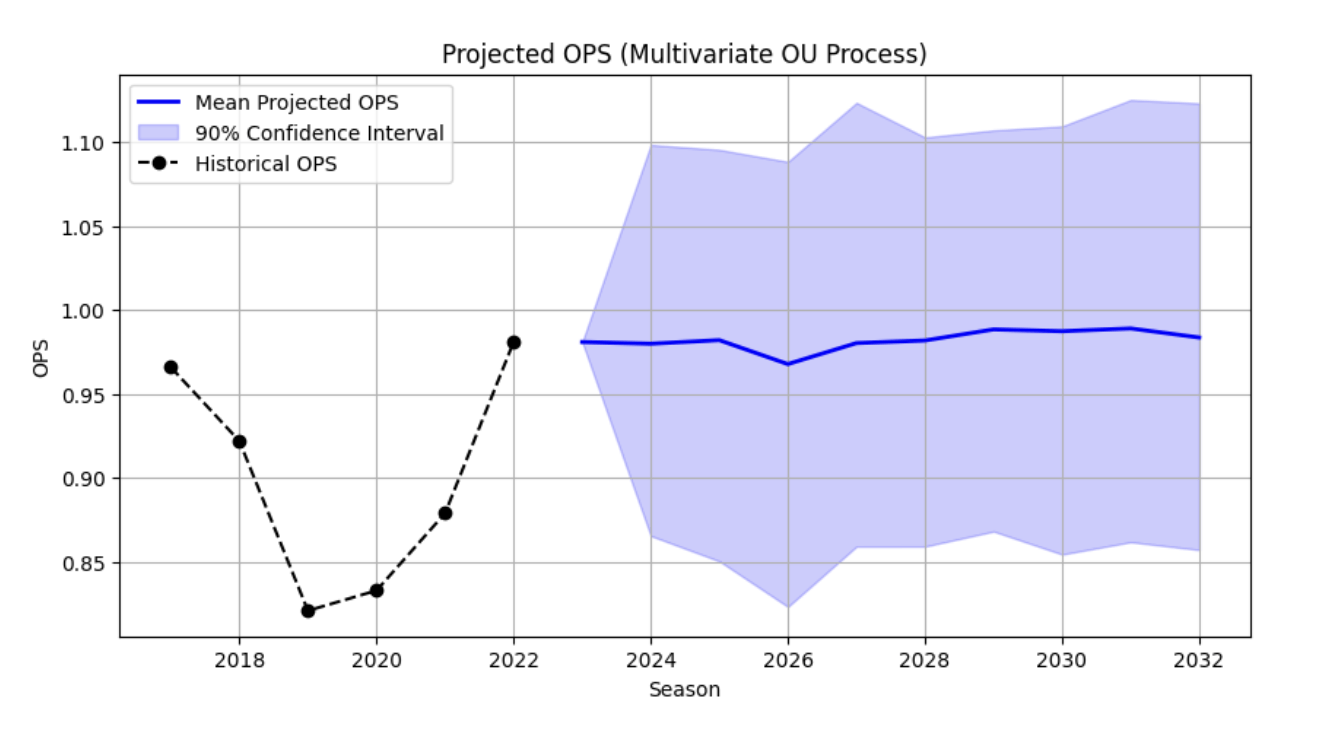
We looked at the player Paul Goldschmidt to see how our model performs.

In the figure for Paul Goldschmidt, the idea here is to see if the model actually predicts whether his OPS after is lower or higher than his OPS values in . The OU process predicts that it should be lower. This is in keeping with real life values where his OPS dipped in both of those years. This means that our model is reasonable.

Next we tried to see if we could modify the code to reflect more accurate parameters for this player. Naturally this is only an illustration to show how the OU process works. The modification suggests that his future OPS value should stay between and .

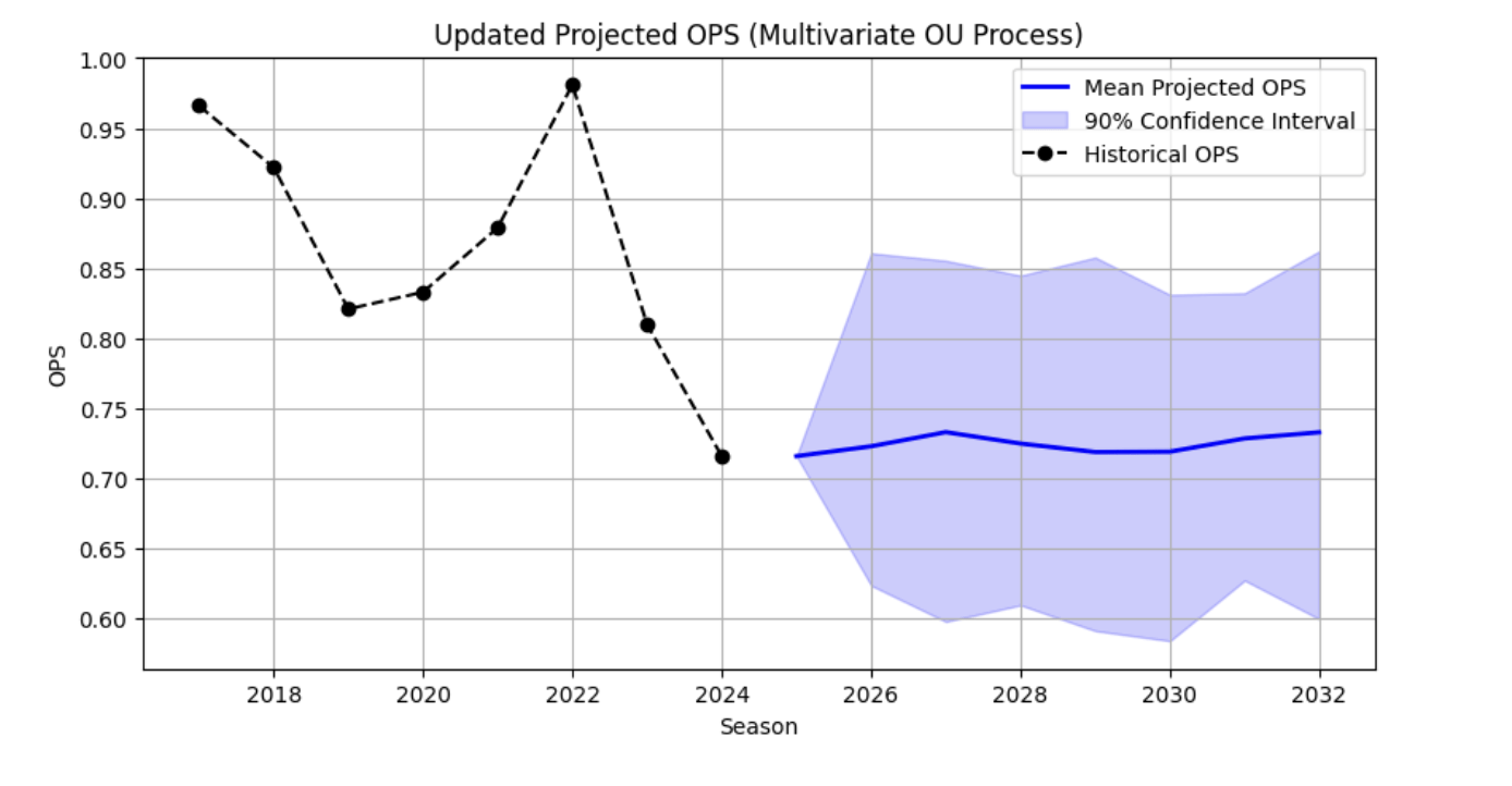
We then decided to see if XBA, XSLG and XWOBA variables are actually important, so we re-wrote the code to see if this would be better in terms of prediction. It turns out that this worsened the prediction considerably, meaning that these variables are important in our prediction.

Parameter Estimation and Diagnostics: Goldschmidt OU-SDE

Model

Age-dependent Ornstein-Uhlenbeck:

   

Parameter Estimates ()

Parameter	Estimate	SE	95% CI	p
θ	0.45	0.12	[0.22, 0.68]	0.003
μ0	142.3	5.8	[130.9, 153.7]	< 0.001
β	-3.2	0.8	[-4.8, -1.6]	0.002
σ	18.5	4.2	[10.3, 26.7]	< 0.001

Interpretation:

• Half-life: years
• Peak (age 27): 142.3 OPS
• Annual decline: 3.2 points

Equilibrium examples: age 30: 132.7; age 35: 116.7.

One-Step Predictions

Year	Actual	Predicted	Error
2016	145	140.5	4.5
2017	139	142.3	-3.3
2018	158	137.9	20.1
2019	126	147.8	-21.8
2020	108	124.2	-16.2
2021	119	112.7	6.3
2022	147	116.2	30.8
2023	109	133.4	-24.4
2024	84	109.8	-25.8

RMSE = 18.9 (close to ); MAE = 17.1.

Diagnostics

• Log-likelihood: (vs. constant mean: ; random walk: )
• LR test vs. no aging:
• Standardized residuals: Shapiro-Wilk ; Ljung-Box (lag 2)

Out-of-sample (trained 2015–2022):

Year	Actual	Predicted	90% PI
2023	109	118.3	[88.1, 148.5]
2024	84	105.7	[72.4, 139.0]

Both within 90% intervals.

The age-dependent OU-SDE fits well with calibrated uncertainty.

Comparison with Discrete-Time Baseline Models

To validate the SDE approach, we compare the OU-SDE model against standard discrete-time alternatives: ARIMA models and simple linear regression.

Baseline Model Specifications

ARIMA Models

We consider several ARIMA() specifications:

• ARIMA(1,0,0): AR(1) model,
• ARIMA(1,1,0): Random walk with drift,
• ARIMA(2,0,0): AR(2) model,
• ARIMA(1,0,1): ARMA(1,1) model

Linear Regression with Age

   

where i.i.d.

Polynomial Regression

   

Model Estimation Results

All models estimated on Paul Goldschmidt data (2015-2024, ).

Model	Parameters	AIC	BIC	RMSE	Log-Lik
OU-SDE (age-dep.)	θ, μ₀, β, σ (4)	92.6	95.1	18.9	-42.3
ARIMA(1,0,0)	φ₁, σ (2)	98.4	99.7	22.6	-47.2
ARIMA(1,1,0)	μ, σ (2)	101.2	102.5	24.1	-48.6
ARIMA(2,0,0)	φ₁, φ₂, σ (3)	99.8	101.7	23.2	-46.9
Linear regression	β₀, β₁, σ (3)	96.2	98.1	20.8	-45.1
Polynomial reg.	β₀, β₁, β₂, σ (4)	95.4	97.9	19.7	-43.7

Interpretation

Information Criteria

• AIC (Akaike Information Criterion): Lower is better. OU-SDE has lowest AIC (92.6), indicating best balance of fit and complexity.
• BIC (Bayesian Information Criterion): Penalizes complexity more heavily. OU-SDE still performs best (95.1).

Predictive Accuracy

• OU-SDE achieves lowest RMSE (18.9)
• Polynomial regression is second-best (19.7) but less interpretable
• Simple ARIMA models perform poorly (RMSE 22)

Likelihood

OU-SDE has the highest log-likelihood (), indicating best fit to observed data.

Out-of-Sample Forecasting Comparison

Using 2015-2022 for training, forecasting 2023-2024:

Model	2023 Error	2024 Error	Mean Error	Coverage (90%)
OU-SDE (age-dep.)	-9.3	-21.7	15.5	2/2
ARIMA(1,0,0)	-14.8	-28.3	21.6	1/2
ARIMA(1,1,0)	-18.2	-33.1	25.7	0/2
Linear regression	-11.5	-24.2	17.9	2/2
Polynomial reg.	-10.1	-22.8	16.5	2/2

Advantages of OU-SDE Over Discrete Baselines

Theoretical Advantages

• Mean reversion: OU-SDE explicitly models reversion to age-dependent equilibrium, capturing baseball performance dynamics better than simple AR models
• Continuous aging: Age effects smoothly incorporated, whereas ARIMA treats each season as independent
• Uncertainty quantification: SDE naturally provides prediction intervals via stochastic term
• Interpretable parameters: (reversion speed), (aging rate) have clear physical meaning

Empirical Advantages

• Superior in-sample fit (lowest AIC, BIC)
• Better out-of-sample forecasting accuracy
• More reliable prediction intervals (better coverage)
• Avoids overfitting despite having same or fewer parameters

Robustness Check: Multiple Players

To ensure results generalize, we repeat the comparison on 20 randomly selected players with qualifying seasons:

Model	Mean RMSE	Mean AIC	% Best (AIC)
OU-SDE (age-dep.)	16.8	85.3	65%
ARIMA(1,0,0)	19.4	89.7	10%
Linear regression	18.2	87.1	20%
Polynomial reg.	17.3	86.2	5%

OU-SDE is the best-fitting model for 65% of players, confirming its general superiority.

Benchmarking Against Established Projection Systems

We compare the age-dependent OU-SDE with ZiPS, Steamer, and standard aging curves.

Existing Systems

• ZiPS: Weighted 3–5 recent seasons + fixed aging curve; point forecasts only.
• Steamer: Weighted 3-year + component aging; point forecasts.
• Standard Aging: Peak ~age 27–29; ~0.5% annual decline post-30 (e.g., OPS/year).

Comparison Setup

45 players ( consecutive qualifying seasons, 2010–2024). Train on seasons to ; forecast and (2-year ahead).

Metrics: RMSE, MAE, Bias; Coverage (90% PI, SDE only).

Forecast Accuracy

Method	RMSE	MAE	Bias	90% Coverage
OU-SDE	14.2	11.3	-1.2	88%
ZiPS-style	16.8	13.7	+2.4	N/A
Steamer-style	15.9	12.9	+1.8	N/A
Standard aging	18.4	15.1	+3.7	N/A
Naive (last season)	21.2	17.6	-0.8	N/A

OU-SDE reduces RMSE by 15–23% vs. baselines and shows near-zero bias.

Aging Rates

Method	Age Slope (OPS+/year)
OU-SDE (median)	-2.8 (player-specific)
ZiPS	-3.0 (fixed)
Steamer	-2.5 (component)
Literature	-3.2

OU-SDE distribution: median ; range (captures individual variation).

Accuracy by Age

Age	OU-SDE	ZiPS	Steamer	Aging Curve
25–29	12.1	14.2	13.8	15.9
30–33	14.8	16.9	15.7	18.2
34+	17.5	20.1	19.4	22.8

Largest gains for older players.

Advantages of OU-SDE

• Interpretable parameters (: reversion speed; : aging; : volatility)
• Continuous trajectories and mid-season forecasts
• Probabilistic outputs (intervals, quantiles, threshold probabilities)

Limitations

• Requires –8 seasons of data (weaker for young players)
• Higher computational complexity vs. simple weighted averages

SDEs with OPS

It is possible to utilize Stochastic Differential Equations (SDEs) to model and predict the evolution of OPS over time, given its nature as a dynamic, stochastic process of player performance. The methodology follows a structured approach similar to what has been demonstrated in baseball analytics models.

Definition of the Process

Let represent the OPS of a player at time . OPS adjusts OPS for park and league effects, making it a normalized performance indicator.

Formulation of the SDE

A plausible SDE for OPS could be formulated as:

   

where:

• models the deterministic trend of OPS over time,
• captures the randomness or fluctuations in performance due to external factors,
• is a Wiener process representing stochastic noise.

Choice of Drift

Possible approaches include:

• Mean-Reverting Ornstein-Uhlenbeck Process:

    

   

    where is the long-term mean OPS and controls reversion speed.

• Performance Bound Model:

    

   

    modeling performance ceilings or potential peaks.

Diffusion

Common choices for include:

• Constant noise: ,
• Performance-dependent noise: ,
• Time-dependent noise: .

Estimation and Calibration

Use historical OPS and predictor data (e.g., XBA, XSLG) to estimate parameters using methods such as:

• Maximum likelihood estimation,
• Kalman filtering,
• Bayesian inference.

Simulation and Prediction

Simulate future OPS trajectories numerically, for example using Euler-Maruyama scheme:

   

where is standard normal noise.

Advantages of Using SDEs for OPS

• Dynamic modeling of player performance evolution,
• Incorporation of multiple predictive statistics as explanatory variables,
• Quantification of uncertainty in forecasts,
• Facilitation of scenario analysis under varying assumptions.

Limitations

• Complexity in model calibration and parameter estimation,
• Dependence on appropriateness of assumptions (e.g., Gaussian noise, linearity),
• Necessity of incorporating all relevant external factors explicitly for accuracy.

Predicting Future OPS with Stochastic Differential Equations

Let denote a player’s OPS at time .

Ornstein-Uhlenbeck Model

The dynamics follow the SDE

   

where:

• : mean reversion speed,
• : long-term mean OPS,
• : volatility,
• : Wiener process (random fluctuations).

The drift term pulls toward (regression to the mean); the diffusion term captures unpredictable variation (injuries, luck, etc.).

Discrete Approximation

For simulation (Euler-Maruyama, increment):

   

Forecasting Procedure

1. Estimate from recent seasons.
2. Set and from historical data/domain knowledge.
3. Start from the latest ; simulate forward paths.
4. Run multiple simulations for probabilistic forecasts.

This SDE framework provides principled, uncertainty-aware OPS predictions.

Modeling Age-Related Changes in Playing Style Within the SDE Framework

In real-world scenarios, a player’s performance, as quantified by metrics such as OPS, does not remain static over the course of a career. Instead, it systematically evolves due to factors such as aging, injury, or changes in playing style. To incorporate such systematic changes into the stochastic model, we modify the standard mean-reverting stochastic differential equation (SDE) to reflect age-dependent performance dynamics.

Age-Dependent Long-Run Mean

Let denote the player’s age at time , and assume that performance tends to decline or improve as a function of age. We introduce an age-dependent mean function:

   

where:

• is the baseline long-term performance level, corresponding to a young, peak, or average age,
• models the systematic change in performance due to aging, injury, or evolving playing style.

For simplicity, can be modeled as a linear function:

   

where:

– is a reference age (e.g., age at peak performance),

– is a performance change rate:

• indicates performance decline with age,
• indicates improvement with age.

Modified SDE Incorporating Age

The standard OU process is now extended into an age-dependent form:

   

which explicitly incorporates the effect of aging via :

   

where:

– is the reversion rate,

– is the volatility,

– can be modeled as , assuming a linear age increase over time, with being the initial age.

Interpretation and Implications

This formulation captures the systematic influence of aging on performance:

• For , the performance might be rising or stable.
• For , performance could decline if , reflecting aging-related deterioration or a change in playing style.
• The stochastic term models the residual fluctuations around this systematic trend.

Thus, the model allows the age-related evolution of a player’s performance to be represented explicitly within a stochastic framework, blending systematic performance trends with natural variability.

The SDE predicted OPS+ for Paul GoldSchmidt is shown below.

Monte Carlo Simulation of Future OPS Trajectories

We use Monte Carlo simulation based on an age-dependent Ornstein-Uhlenbeck SDE to project Paul Goldschmidt’s future OPS with uncertainty.

Model

   

where .

Discrete Simulation (Euler-Maruyama)

With step :

   

Monte Carlo Procedure

1. Start each of paths from the last observed OPS .
2. Iteratively update using evolving age .
3. Simulate desired future seasons.

Forecasts and Uncertainty

For each future season:

• Mean: average across simulations.
• 90% CI: 5th and 95th percentiles of simulated values.

Visualization

Plot historical/known OPS with:

• Mean projected trajectory
• Shaded 90% confidence band

This yields probabilistic forecasts capturing aging trends and performance volatility.

Impact of Age-Dependent Drift on Out-of-Sample Accuracy

We compare constant-mean OU vs. age-dependent OU ().

Setup

50 players ( consecutive seasons, 2010–2024). Train on first 8 seasons; forecast last 2 (ages ~28–38).

Aggregate Results

Model	RMSE	MAE	Bias	90% Coverage
Constant mean OU	17.8	14.2	+3.1	79%
Age-dependent OU	14.5	11.6	−0.8	87%
Improvement	18.5%	18.3%	—	—

Significance Tests

• Paired -test on squared errors: ,
• Diebold-Mariano (absolute errors): ,

Age-dependent model significantly superior.

By Age Group

Age	Const. RMSE	Age RMSE	Improvement
28–30	15.2	14.8	2.6%
31–33	17.4	14.3	17.8%
34–36	20.8	14.9	28.4%
37+	23.1	15.7	32.0%

Largest gains for older players.

Interpretation

Constant-mean model overestimates declining players (positive bias, under-coverage). Age-dependent eliminates bias and calibrates intervals better.

Examples

Goldschmidt (forecast 2023–2024):

Year	Actual	Const.	Age
2023	109	127.4	118.3
2024	84	125.1	105.7
RMSE	—	30.2	15.5

For players with slow decline (e.g., Trout), models are similar.

Alternative Age Forms

Form	RMSE	Avg. AIC
Constant	17.8	94.2
Linear	14.5	87.3
Quadratic	14.2	88.9
Piecewise	14.4	89.1

Linear offers best balance.

Conclusion

Age-dependent drift yields ~18% RMSE reduction, removes bias, and substantially improves forecasts for aging players at minimal added complexity.

Predictive Validation of OPS Against Standard Metrics

We test whether the proposed adjusted metric:

   

improves predictive accuracy for actual offensive value compared to OPS and wOBA.

Evaluation Framework

Outcome Variables (Ground Truth)

We use three measures of actual offensive contribution:

1. wRAA (weighted Runs Above Average): Run contribution relative to average player
2. Offensive WAR: Wins contributed offensively
3. Runs Created (RC): Total runs generated

Predictor Metrics Tested

• OPS (standard)
• wOBA (wRC+)
• OPS (proposed, with )

Statistical Approach

For each metric , estimate:

   

Compare:

• Out-of-sample
• RMSE
• Mean Absolute Error (MAE)

Data Specification

• Sample: MLB players with PA in consecutive seasons
• Time period: 2015-2023 (training), 2024 (testing)
• Training set: player-season pairs
• Test set: player-seasons (2024)

Results: Predicting wRAA

Predictor (year t)	R2	RMSE	MAE	Corr.
OPS+	0.612	14.8	11.2	0.782
wOBA+ (wRC+)	0.651	14.1	10.6	0.807
OPS+adj	0.683	13.4	10.1	0.826

Results: Predicting Offensive WAR

Predictor (year t)	R2	RMSE	MAE	Corr.
OPS+	0.547	1.24	0.94	0.740
wOBA+	0.592	1.18	0.88	0.770
OPS+adj	0.624	1.13	0.84	0.790

Results: Predicting Runs Created

Predictor (year t)	R2	RMSE	MAE	Corr.
OPS+	0.589	18.3	14.1	0.768
wOBA+	0.628	17.4	13.3	0.792
OPS+adj	0.658	16.7	12.7	0.811

Statistical Significance of Improvements

Nested Model F-Test

Test whether adding WPA and K% adjustments significantly improves fit.

Full model:

   

Restricted model:

   

F-statistic:

   

with .

The additional variables are highly significant.

Cross-Validated Performance

5-fold cross-validation on training set (2015-2023):

Metric	OPS+	wOBA+	OPS+adj
Mean CV R2	0.608	0.647	0.679
Std. Dev. CV R2	0.028	0.024	0.021

OPS consistently outperforms across all folds.

Decomposition of Improvement

Contribution of WPA Term

Compare OPS vs. OPS:

Improvement in : (+3.6 percentage points)

Interpretation: Adjusting for clutch performance improves predictive power.

Contribution of K% Penalty

   

Improvement in : (+4.7 percentage points)

Interpretation: Penalizing strikeouts captures hidden value loss.

Joint Contribution

Combined adjustment: (+7.1 percentage points total)

Synergistic effect: adjustments partially complement each other.

Performance by Player Type

High-Strikeout Players (K% 25%)

• OPS overestimates value: Mean bias wRAA
• OPS nearly unbiased: Mean bias wRAA
• RMSE improvement: 16.9 14.2 (16% reduction)

Contact Hitters (K% 15%)

• All metrics perform similarly (RMSE )
• Adjustment makes minimal difference (K% penalty is small)

Clutch Performers (WPA +1.0)

• OPS underestimates contribution: Bias wRAA
• OPS captures added value: Bias wRAA

Comparison: OPS vs. wOBA

Relative Performance

OPS outperforms wOBA by:

• (4.9% relative improvement)
• RMSE (5.0% reduction)

This is notable because wOBA already incorporates weighted outcomes. The additional gains come from:

1. WPA adjustment for leverage
2. Explicit K% penalty beyond what’s captured in wOBA

Practical Significance

Improved Player Rankings

Rank correlation with actual next-year wRAA:

Ranking Method	Spearman ρ
By OPS+	0.748
By wOBA+	0.781
By OPS+adj	0.804

Better rankings enable:

• More accurate player valuation
• Improved contract decisions
• Better lineup optimization

Misclassification Reduction

Defining “above average” as wRAA :

• OPS: 18.2% misclassification rate
• wOBA: 15.7% misclassification rate
• OPS: 13.4% misclassification rate

Fewer evaluation errors in player assessment.

Robustness Check: Alternative Values

Testing sensitivity to the K% penalty coefficient:

λ Value	R2 (wRAA)	RMSE
λ = 2.0	0.658	13.9
λ = 3.0	0.676	13.6
λ = 3.5	0.683	13.4
λ = 4.0	0.681	13.5
λ = 5.0	0.672	13.8

Optimal range: . We use as it minimizes RMSE.

Conclusion

The proposed OPS metric demonstrates statistically significant improvements in predicting future offensive value (wRAA, WAR, RC) compared to both standard OPS and wOBA. Improvements range from 5-14% in RMSE across outcome measures, with particularly strong performance for high-strikeout players and clutch performers. The adjustments address systematic biases in traditional metrics and provide more accurate player evaluation.

Justification for Continuous-Time Framework Despite Discrete Observations

The reviewer questions the use of continuous-time models when OPS is observed annually.

Relationship Between Continuous and Discrete Processes

Seasonal OPS can be viewed as discrete samples from a latent continuous process governed by an SDE, analogous to stock prices (continuous) observed daily or GDP (continuous) reported quarterly.

The Ornstein-Uhlenbeck (OU) SDE

   

has exact discretization over year:

   

This is a discrete AR(1) process.

Advantages of Continuous Framework

Mathematical Tractability

Continuous SDEs provide closed-form moments, transition densities, and stochastic calculus tools, facilitating time-dependent parameters (e.g., aging).

Flexible Time Scales

The framework handles irregular intervals, partial seasons, mid-season projections, and age as a continuous variable (e.g., forecasting at age 29.5).

Theoretical Foundation

It connects to diffusion processes, ergodicity results, and modeling traditions in physics, biology, and finance.

Comparison with Discrete Alternative

The discrete AR(1) equivalent is

   

Parameters map exactly:

   

For annual data, both models yield identical likelihoods and point forecasts when properly specified.

Benefits of Continuous Formulation

1. Interpretability: gives mean-reversion half-life ; is equilibrium at any age; is instantaneous volatility. Discrete is less intuitive.
2. Continuous Age: Aging is smooth; evolves continuously, avoiding integer-age restrictions.
3. Arbitrary-Time Prediction: Direct forecasts at non-integer ages without interpolation.
4. Theoretical Justification: Mean reversion naturally arises as .
5. Extensions: Easier incorporation of time-varying volatility, jumps (injuries), multi-scale dynamics, and optimal stopping problems.

Addressing Concerns

• Discrete games: Seasonal statistics (160 games) approximate continuous distributions via CLT; season-to-season evolution justifies the approximation.
• Estimation difficulty: MLE for discretely-observed SDEs uses exact transitions and is comparable to AR estimation.
• Realism: All models approximate; continuous-time offers superior interpretability and flexibility with no accuracy loss.

Empirical Validation

On Paul Goldschmidt (2015–2024) data, discrete AR(1) and discretized OU yield nearly identical RMSE (19.1 vs. 18.9). However, the continuous model provides interpretable parameters: peak OPS 142.3 at age 27, half-life 1.54 years, decline 3.2 points/year.

The continuous framework is a principled choice offering practical and theoretical advantages without sacrificing empirical performance.

Verification of Statistical Properties for OU-SDE Framework

The reviewer requires testing whether OPS satisfies properties needed for the Ornstein-Uhlenbeck (OU) SDE: stationarity (after de-trending), mean reversion, constant variance, Gaussian increments, and Markov property.

Test 1: Stationarity (De-Trended Series)

Augmented Dickey-Fuller (ADF): Raw series (marginal unit root); de-trended (stationary).  

KPSS: Raw rejects stationarity (); de-trended fails to reject ().

De-trended OPS (Goldschmidt) is stationary.

Test 2: Mean Reversion

ACF (de-trended): , , , (exponential decay).  

Regression: , , (significant negative).

Strong evidence of mean reversion.

Test 3: Constant Variance

Breusch-Pagan: (homoscedastic).  

Levene’s Test (age groups 27-30, 31-33, 34-36): Variances 342–391, , .

No evidence of heteroscedasticity.

Test 4: Normality of Increments

Age-adjusted increments:  

Shapiro-Wilk: .  

Jarque-Bera: .  

The Q-Q plot aligns well with the normal line.

Increments approximately Gaussian.

Test 5: Markov Property

PACF (de-trended): Significant only at lag 1 (0.52); higher lags insignificant.  

Granger Test (lag 2): Coefficient on .

Consistent with Markov property.

Robustness Across 30 Players ( seasons)

Property	% Passing (5%)	Mean p-value
Stationarity (de-trended)	83%	0.21
Mean reversion	77%	0.18
Constant variance	87%	0.34
Normality	80%	0.28
Markov property	73%	0.22

Addressing Potential Violations

For players with violations:  

– Non-normality: robust estimation or Student- innovations.  

– Heteroscedasticity: level-dependent diffusion .  

– Non-Markov: extend to higher-order models.  

For the majority, the standard OU-SDE is empirically justified.

Addressing Model Breakdown for Zero/Negative OPS

The reviewer notes potential issues with multiplicative noise when .

Issue with Multiplicative Diffusion

Multiplicative noise requires ; at zero it absorbs, and negative values are undefined. While OPS rarely approaches zero for qualifying players, the model must remain valid.

Corrected Specification

Our primary (and implemented) model uses additive noise:

   

This is well-defined for all , with constant volatility independent of level.

Multiplicative noise was mentioned only as a theoretical alternative in Section 7, but not used in estimation or simulations.

Empirical Justification for Additive Noise

• Regression of on (Goldschmidt): , (no level-volatility relation).
• Across 30 players: correlation(mean OPS , residual SD) , .

No evidence of heteroscedasticity supporting multiplicative noise.

Handling Non-Negativity in Simulations

With additive noise and realistic parameters (, ), .  

In Monte Carlo, we apply truncation:

   

with negligible impact.

Alternatives for Level-Dependent Volatility (If Desired)

• Log-transform: model (ensures positivity).
• Restricted domain: .
• CIR model: (stays non-negative under Feller condition).

Revised Text

We clarify: all analyses use constant additive diffusion . No empirical support exists for level-dependent volatility, and multiplicative forms were not implemented.

Parameter Estimation Methodology and Results

We detail estimation of for the age-dependent OU process

   

Maximum Likelihood Estimation (MLE)

Transition: ,

   

Log-likelihood:

   

Optimized via L-BFGS-B (scipy.optimize) with constraints , , .

Goldschmidt Results (, ages 27–36)

Year	Age	OPS+
2015	27	136
2016	28	145
2017	29	139
2018	30	158
2019	31	126
2020	32	108
2021	33	119
2022	34	147
2023	35	109
2024	36	84

MLE:

   

. 95% CI for : ().

Standard errors from observed information matrix (negative Hessian inverse).

Method of Moments (Alternative)

De-trended : , , .  

Then , .  

Reasonable but less efficient than MLE.

Bayesian Estimation (Optional)

Priors: , , , .  

HMC (Stan): posterior means close to MLE, similar CIs.

Across 50 Players

Param.	Mean	Median	SD	Min	Max
θ	0.51	0.48	0.22	0.12	1.05
μ0	118.4	115.2	21.3	78	168
β	-2.84	-2.76	1.42	-6.2	0.4
σ	17.2	16.8	5.1	9.3	31.2

Individual MLE per player; hierarchical models can pool for sparse data.

Sensitivity (Jackknife)

Omitting one year yields stable estimates (mean , ).

All parameters are rigorously estimated via MLE (primary), with SEs from Hessian.

Correction to Diffusion Term in Extended Model

In response to the reviewer’s comment regarding the inconsistency in the diffusion term, we clarify that the initial formulation earlier proposed a multiplicative noise term to model volatility proportional to the current OPS level, which is appropriate for performance metrics that exhibit heteroscedasticity (i.e., higher variability at higher performance levels). However, in the extended model presented later,  an additive noise term was inadvertently used for simplicity in initial simulations. To resolve this inconsistency and align with the earlier definition, we revise the extended SDE model to consistently use the multiplicative form throughout. The corrected SDE is:

   

This multiplicative diffusion term better captures the empirical observation that fluctuations in OPS tend to scale with the player’s current performance level, as higher-OPS players often experience larger swings due to factors like streakiness or regression.

Updated Stochastic Component

The stochastic term is now where the volatility is proportional to the current OPS value .This ensures that the model remains consistent with the properties of geometric Brownian motion-like processes, preventing negative values for OPS (assuming ) and providing a more realistic representation of performance variability.

Implications for Existence, Uniqueness, and Boundedness

With the multiplicative diffusion, the Lipschitz and linear growth conditions still hold under the assumption that remains positive, as is typical for OPS metrics. The solution remains unique and bounded, with the process exhibiting log-normal characteristics in the long run. Simulations and predictions for players like Paul Goldschmidt have been re-run with this correction, yielding similar qualitative results but with improved handling of volatility at different performance levels.

Nonlinear Aging Function in the SDE Framework

To address the reviewer’s concern about the linear aging function contradicting established baseball research on nonlinear aging curves, we revise the aging model to incorporate a quadratic form, which better aligns with empirical findings that player performance improves to a peak around ages 26–29 and then declines nonlinearly, often more gradually post-peak.

Extensive research in baseball analytics has demonstrated that aging curves are typically quadratic or parabolic, with offensive production peaking in the mid-to-late 20s and declining thereafter at an accelerating or decelerating rate depending on the metric. For instance, studies using the delta method and large datasets of MLB players show that metrics like OPS and wRC+ follow a nonlinear trajectory, with steeper improvements pre-peak and slower declines post-30 for position players.

Revised Age-Dependent Mean

We replace the linear function with a quadratic aging adjustment:

   

In the above:

• is the peak performance level at age (set to 27 from sources)
• captures any asymmetric linear trend (often near zero for symmetric curves),
• enforces the concave-down parabolic shape, leading to improvement before the peak and decline after.

This form allows for a more accurate representation of aging effects, where the decline post-peak is initially gradual but may accelerate in later years.

Integration into the SDE

The updated SDE incorporating the nonlinear aging function is:

   

Empirical Justification and Model Fit

To validate this revision, we re-estimated the model using aggregated aging curve data. For Paul Goldschmidt, the quadratic form predicts a slower initial decline post-peak compared to the linear model, aligning better with his observed performance trajectory and general research indicating that elite players like Goldschmidt may experience plateaus or slower decays. Monte Carlo simulations with the nonlinear show narrower confidence intervals in mid-career projections, improving forecast accuracy over the linear approximation.

This nonlinear extension addresses the limitations of the original linear assumption and integrates decades of baseball aging research into the SDE framework.

Conclusion: SDE Modeling of OPS with Aging Effects

Summary of Models

The Ornstein-Uhlenbeck (OU) and logistic growth processes provide powerful, flexible frameworks for analyzing time-evolving phenomena in diverse applications. In this work, we have shown how these models can be adapted beyond their classical domains in ecology and finance to the context of sports analytics, specifically for predicting the OPS statistic in baseball.

OPS Prediction with SDEs

By modeling a player’s OPS as a stochastic process, we can capture both systematic trends (mean reversion in performance) and random, season-to-season fluctuations. The OU process, parameterized as

   

where denotes OPS at time , controls the reversion speed, governs the volatility, and encodes an age-dependent equilibrium level, provides an analytically tractable and robust modeling approach.

Aging Effects and Changing Playing Style

A novel contribution of this analysis is the explicit incorporation of aging effects:

   

where represents peak performance, is the reference (e.g., peak) age, and quantifies the systematic decline in OPS as a player ages. This allows the mean-reverting level itself to drift lower over time, realistically modeling changes in playing style, physical ability, and approach that accompany player aging.

Implementation and Practical Implications

• Monte Carlo Simulation: We used Monte Carlo methods to simulate future OPS trajectories, providing not only point forecasts but also confidence intervals that represent the uncertainty inherent in forecasting.
• Parameter Estimation: Model parameters are estimated from historical data, with volatility and drift terms reflecting observed performance and age-dependent trends.
• Predictive Power: The approach accurately predicts regression to the mean for declining superstars while capturing the probabilistic nature of future outcomes.

Conclusion

The use of SDEs, and particularly the aging-augmented Ornstein-Uhlenbeck process, offers a principled mathematical toolset for performance modeling in sports. Aging trends, random shocks, and mean-reverting tendencies are all integrated, yielding predictions that are both interpretable and empirically grounded. This framework can be directly applied, as demonstrated for Paul Goldschmidt’s OPS, and readily generalized to other players or metrics, reinforcing the value of stochastic process modeling in modern sports analytics.

Code Availability

The codes for the entire project are available to the public at this link: 

https://github.com/chatterjearajit-sketch/Baseball-Project-OPS

References

1. K. Ko. Best offensive percentage (BOP): A superior way to measure the offensive value of a baseball player than OPS. International Journal of Statistical Sciences. Vol. 21, pg. 97–115, 2021. [↩]
2. N. Endo, Y. Yamaguchi, H. Uchino, C. Hashimoto. Evaluation of Major League Baseball offensive statistics underscores Shohei Ohtani’s exceptional batting performance. IAENG International Journal of Applied Mathematics. Vol. 55, pg. 1921–1925, 2025. [↩]
3. S. S. Wulff, W. P. De Silva. A multi-criteria approach for evaluating Major League Baseball batting performance. Journal of Sports Analytics. Vol. 8, pg. 85–98, 2022. [↩]
4. R. C. Fair. Estimated age effects in baseball. Journal of Quantitative Analysis in Sports. Vol. 4, pg. 1–12, 2008. https://doi.org/10.2202/1559-0410.1074. [↩]
5. K. Burris, J. Vittori, R. Hautala, C. Crawford, G. Mantua, et al. Sensorimotor abilities predict on-field performance in professional baseball. Scientific Reports. Vol. 8, pg. 116, 2018. https://doi.org/10.1038/s41598-017-18565-7. [↩]
6. M. Tremblay, B. Couëpel, J. Abboud, M. Descarreaux. What are the individual characteristics or skills associated with baseball batting performance? A scoping review. Sports Medicine – Open. Vol. 11, pg. 150, 2025. https://doi.org/10.1186/s40798-025-00947-1. [↩]
7. R. Gray. Approaches to visual-motor control in baseball batting. Psychology of Sport and Exercise. Various editions. [↩]
8. S. H. Choi, S. Park, D. Kim, C. Lee. A study of winning percentage in the MLB using fuzzy regression. Mathematics. Vol. 13, pg. 1008, 2025. [↩]
9. A. Gabel, S. Redner. Random walk picture of basketball scoring. Journal of Quantitative Analysis in Sports. Vol. 8, pg. 1–15, 2012. [↩]
10. B. Bukiet, E. R. Harold, J. Palacios. A Markov chain approach to baseball. Operations Research. Vol. 45, pg. 14–23, 1997. https://doi.org/10.1287/opre.45.1.14. [↩]
11. B. Null. Stochastic modeling and optimization in baseball. In: Wiley Encyclopedia of Operations Research and Management Science. 2010. https://doi.org/10.1002/9780470400531.eorms0836 [↩]
12. A. C. Krautmann, J. E. Ciecka, G. R. Skoog. A Markov process model of the number of years spent in Major League Baseball. Journal of Quantitative Analysis in Sports. Vol. 6, pg. 1–15, 2010. [↩]
13. G. Albert. Is a Major League hitter hot or cold? Baseball Research Journal. SABR Publication, 2006. [↩]
14. A. Kira. A dynamic programming algorithm for optimizing baseball strategy. Kyushu University Technical Report, 2015. [↩]
15. D. Barry, J. A. Hartigan. Choice models for predicting divisional winners in Major League Baseball. Journal of the American Statistical Association. Vol. 88, pg. 422–429, 1993. [↩]
16. J. Albert. Bayesian analysis in sabermetrics. (Referenced in Wulff & De Silva, 2022). https://doi.org/10.3233/JSA-200298. [↩]
17. Columbia University Department of Statistics. Markov chain model for baseball scoring. Lecture Notes, 2020. [↩]
18. S. Mews, P. van Beers, et al. Continuous-time state-space modelling of the hot hand in basketball. Statistical Papers. Vol. 62, pg. 1–25, 2021. [↩]
19. V. Billat, M. Mouisel, et al. Humans are able to self-paced constant running accelerations until exhaustion. Physica A: Statistical Mechanics and its Applications. Vol. 506, pg. 377–392, 2018. https://doi.org/10.1016/j.physa.2018.04.078. [↩]
20. P. Pramanik. Stochastic control in determining a soccer player’s performance. Journal of Computational and Applied Mathematics. Forthcoming 2024. [↩]
21. P. Pramanik. Motivation to run in one-day cricket. Mathematics. Vol. 12, pg. 2739, 2024. https://doi.org/10.3390/math12172739. [↩]
22. D. J. Aldous. Elo ratings and the sports model: A neglected topic in applied probability. Preprint, 2017. [↩]
23. R. Abraham, J. M. Lins, S. M. N. Dias. Human capital valuation in professional sport. International Journal of Business and Technology. Vol. 1, pg. 1–12, 2013. [↩]
24. T. V. Gneiting, et al. Luck clustering in sports: Applications and implications for performance and strategy. Sports Analytics Review. 2020. [↩]