NHSJS

Path Signatures for Regime Detection in Cryptocurrency Markets: A Rough-Path Framework Using Spot, Perpetual Basis, and Funding Rates

August 20, 2026

Abstract

Background. Cryptocurrency markets exhibit fast, reflexive regime transitions driven by leverage cycles, coordinated liquidations, and perpetual-swap funding imbalances. Classical regime-detection methods — hidden Markov models (HMMs) on returns and rolling-volatility thresholds — impose Markovian dynamics and summarize path information through low-dimensional moments, missing the path-dependent structure of crypto regime shifts.
Methods. We develop a regime-detection framework based on truncated path signatures from rough-path theory. We construct a multivariate path of BTC and ETH log-returns, a realized-volatility proxy, perpetual-spot basis, and 8-hour funding rates, with lead-lag and time augmentation. Truncated signatures of depth N=3 are extracted from rolling 168-hour windows, robust-scaled, projected to 128 components by truncated SVD, and passed to ℓ2-penalized logistic regression. We prove a universal-approximation result establishing signatures as a rich feature family for continuous path functionals, and separately discuss what this implies for supervised regime classification. We benchmark against four baselines — univariate HMM, multivariate HMM, rolling-volatility tercile, and HAR-RV — with purged walk-forward validation, a 168-hour embargo between train and test folds, and block-bootstrap 95% confidence intervals.
Results. Signature methods are competitive with the strongest baseline (HAR-RV) on forward-volatility tercile classification across horizons 24h, 72h, and 168h, and produce the highest test accuracy at the 168h horizon. On average precision for prospective detection of top-decile forward volatility events over the full 2023–2026 test timeline, SIG-LR outperforms all baselines. In an event study across six canonical regime shifts, signatures produce the cleanest event-localized probability signals: signatures detect the out-of-sample SVB/USDC depeg within a 4-hour window of the event core across all tested thresholds and correctly abstain on the bullish BTC ETF approval. The signature advantage localizes empirically in third-order iterated integrals dominated by cross-coordinate interactions involving basis and realized-volatility coordinates. Signatures do not solve directional return prediction at sub-daily horizons, consistent with market-efficiency expectations.
Conclusions. Path signatures are a competitive feature representation for crypto regime detection whose primary practical advantage is not headline predictive accuracy but interpretable, event-localized signal cleanliness with a clear financial interpretation of the driving coordinates.

Keywords: rough path theory, path signatures, regime detection, cryptocurrency, perpetual futures, funding rates, hidden Markov models, universal approximation, walk-forward validation.

Introduction

Cryptocurrency markets have, over the past decade, matured into a liquid, globally accessible, continuously-traded asset class. Daily spot turnover on the largest centralized exchanges regularly exceeds fifty billion U.S. dollars, and notional open interest in perpetual futures on Bitcoin and Ether often surpasses the corresponding cash-settled equity-index contracts traded on CME. Despite this scale, the statistical behavior of crypto returns is markedly distinct from that of traditional financial assets. Unconditional volatility runs three to five times that of large-capitalization equities, return distributions exhibit heavier tails, trading runs continuously across the week, and the market microstructure features deep perpetual-swap order books in which leverage is directly observable through exchange-reported funding rates and open-interest series.

These differences reflect a qualitative change in price-formation dynamics. Whereas equity regime shifts typically propagate through earnings cycles or macroeconomic narratives, crypto regime shifts are frequently reflexive: a change in aggregate leverage positioning precipitates a forced-liquidation cascade, which alters the price path, which feeds back into positioning. The collapses of Terra-LUNA in May 2022 and FTX in November 2022 are canonical examples. In both cases, the transition from a stable regime into acute distress occurred on timescales of hours, and the statistical signatures of the coming transition were visible in the joint dynamics of spot, basis, and funding well before they registered in any univariate volatility summary. Detecting such regime shifts ex ante or with minimal ex-post lag is consequential for risk desks, prime brokers, portfolio managers, and execution algorithms¹^,² .

The standard toolkit for regime detection in financial time series rests on assumptions that are violated in this setting. Hidden Markov models, introduced in their economic form by Hamilton³ , posit an unobservable discrete state evolving as a Markov chain; their inference machinery is mature⁴^,⁵^,⁶ and widely implemented. Rolling-window statistics on realized volatility provide nonparametric threshold detectors that are standard on practitioner trading desks⁷^,⁸ . Heterogeneous autoregressive (HAR) models on realized volatility remain the workhorse for daily and multi-day volatility forecasting in the empirical literature. All of these methods are either Markovian or memoryless with respect to path shape, or they compress multivariate path information into moments computed over trailing windows.

A mathematically principled response is provided by the theory of rough paths⁹^,¹⁰^,¹¹ . Given a continuous path X:0,TRd of finite p-variation, the signature of X is the infinite sequence of iterated integrals over the path, valued in the tensor algebra. The construction dates to Chen for smooth paths¹² and was extended by Lyons to paths of arbitrary finite p-variation. Signatures encode an infinite collection of order-aware interactions between coordinates and are, under mild conditions, near-injective on the space of paths¹³ . Linear functionals of truncated signatures are dense in the space of continuous functionals on compact sets of paths¹⁴^,¹⁵^,¹⁶ , and efficient implementations¹⁷^,¹⁸ make signature feature extraction tractable for large datasets on commodity hardware.

Signature methods have proliferated in quantitative finance, including high-frequency equity prediction¹⁹ , optimal execution²⁰ , signature-based stochastic models²¹ , market simulation²² , and volatility modeling²³^,²⁴^,²⁵ . Most directly relevant, Horvath and Issa²⁶ develop a non-parametric online regime-detection method using signatures within a maximum-mean-discrepancy two-sample test. A rough-volatility perspective on Bitcoin²⁷^,²⁸ establishes that crypto log-volatility is substantially rougher than equity benchmarks, providing motivation for path-based methods. Existing regime-switching models for crypto²⁹^,³⁰ do not leverage multivariate perpetuals data or path-dependent feature representations.

This paper develops a treatment of signature-based regime detection in cryptocurrency markets with the following contributions. First, we construct a crypto-native multivariate path combining time, BTC and ETH log-prices, a realized-volatility proxy, perpetual-spot basis, and hourly funding rates, augmented with lead-lag embedding³¹ and time augmentation. Basis and funding are directly observable measures of leverage positioning unavailable in equity markets and, to our knowledge, have not previously appeared as signature coordinates. Second, we prove a universal-approximation result for continuous path functionals by linear functionals of truncated signatures, and we separately discuss what this theoretical result does and does not imply for supervised regime classification — an important distinction in noisy, non-stationary market environments. Third, we conduct a purged walk-forward evaluation with a 168-hour embargo between train and test folds, block-bootstrap 95% confidence intervals on all reported metrics, and comparison against HAR-RV in addition to standard HMM baselines. Fourth, we perform ablations across signature truncation depths (N=2,3), SVD component counts (32, 128, 512), and feature-set variants (with and without realized volatility). Fifth, we perform an event study across six canonical regime shifts and evaluate detection via a prospective precision-recall analysis on the full test timeline with an ex-ante-defined event label.

Our headline finding is nuanced. Signatures are competitive with the strongest baseline (HAR-RV) on aggregate accuracy across horizons and lead on accuracy at the 168-hour horizon, but the confidence intervals overlap substantially with HAR-RV and rolling-volatility baselines at shorter horizons. The primary practical advantage of signatures is not headline predictive accuracy but event-localized signal cleanliness with interpretable financial mechanism: signatures produce the tightest detection windows at distress events and correctly discriminate distress-driven from bullish-regime volatility, and the top-coefficient signature coordinates are dominated by interactions among basis and realized-volatility channels, matching the leverage-cycle intuition that motivated the framework.

Methods

Notation

Symbol	Meaning
$T$	Time horizon (window length)
$d$	Ambient dimension of the raw path
$d_{\mathrm{aug}}$	Dimension of the augmented (lead-lag, time-augmented) path
$X:[0,T]\to\mathbb{R}^d$	A continuous path
$\\|X\\|_{p\text{-var},[s,t]}$	p-variation of X over [s,t]
$BV_p([0,T];\mathbb{R}^d)$	Banach space of continuous paths of finite p-variation
$T\left((\mathbb{R}^d)\right)$	Tensor algebra over Rd
$T^N\left((\mathbb{R}^d)\right)$	Truncated tensor algebra at depth N
$S(X)_{s,t}$	Signature of path X over interval [s,t]
N	Projection onto truncated tensor algebra of depth N
$D_N$	Dimension of truncated signature at depth N
$K$	Compact set of paths
$L:K\to\mathbb{R}$	Continuous target functional
$M$	Diameter of K in 1-variation
$\gamma_t$	Filtered HMM posterior at time t
$b_t^i, f_t^i$	Perpetual-spot basis and funding rate for asset i at time t
$r_t^i, v_t$	Log-return of asset i and 24h realized-vol proxy at time t

Table 1 | Summarizes the notation used throughout the manuscript.

Mathematical framework

Fix a horizon $T>0$ and dimension $d\geq1$ . A path is a continuous map $X:[0,T]\to\mathbb{R}^d$ . For a partition $\pi={0=t_0<\cdots<t_n=T}$ and $p\geq1$ , the $p$ -variation of $X$ on $[s,t]\subseteq[0,T]$ is

$|X|_{p\text{-var},[s,t]} = \left(\sup_{\pi}\sum_i |X_{t_{i+1}}-X_{t_i}|^p\right)^{1/p}.$

Denote by $BV_p([0,T];\mathbb{R}^d)$ the Banach space of continuous paths of finite $p$ -variation.

The tensor algebra over $\mathbb{R}^d$ is $T\left((\mathbb{R}^d)\right) = \bigoplus_{k\geq0}(\mathbb{R}^d)^{\otimes k}$ . Fix an orthonormal basis ${e_1,\ldots,e_d}$ of $\mathbb{R}^d$ . For $X\in BV_1([0,T];\mathbb{R}^d)$ , the signature of $X$ on $[s,t]$ is

$\begin{equation*}S(X){s,t} = (1, S{s,t}^1, S_{s,t}^2, \ldots),\end{equation*}$

$\begin{equation*} S_{s,t}^k(X) = \idotsint\limits_{s<t_1<\cdots<t_k<t} dX_{t_1}\otimes\cdots\otimes dX_{t_k}.\end{equation*}$

Signature coordinates encode order-aware interactions. The $(i,j)$ – and $(j,i)$ -coordinates of level 2 differ in general, and their difference equals twice the signed L’evy area of the projection of $X$ onto the $(X^i,X^j)$ -plane.

Proposition 1 (Factorial decay). For $X\in BV_1([0,T];\mathbb{R}^d)$ and all $k\geq0$ ,

$|S_{s,t}^k(X)| \leq \frac{|X|_{1\text{-var},[s,t]}^k}{k!},$

where $|\cdot|$ is the Hilbert-Schmidt norm.

Proof. Let $\omega(s,t)=|X|_{1\text{-var},[s,t]}$ . By Fubini and the definition of the iterated integral,

$|S_{s,t}^k(X)| \leq \idotsint\limits_{s<t_1<\cdots<t_k<t} |dX_{t_1}|\cdots|dX_{t_k}| = \frac{\omega(s,t)^k}{k!},$

with the $1/k!$ factor arising from the volume of the ordered simplex.

For our data with per-window 1-variation $M\approx0.5$ , truncation at $N=3$ retains approximately 99.7% of the signature norm and $N=4$ retains essentially all of it.

Two algebraic identities make signatures computationally tractable. Chen’s identity¹² : for $0\leq s\leq u\leq t\leq T$ , $S(X){s,t}=S(X){s,u}\otimes S(X)_{u,t}$ . The shuffle identity³² : for multi-indices $I,J$ , $\langle S(X),e_I\rangle\cdot\langle S(X),e_J\rangle = \sum_{K\in I\shuffle J}\langle S(X),e_K\rangle$ . The shuffle identity implies that linear functionals of the signature form a polynomial algebra: linear regression on signatures realizes polynomial regression on path coordinates.

Two augmentations enhance signature expressivity. Time augmentation replaces $X$ with $(t,X_t^1,\ldots,X_t^d)$ ; the strictly monotone first coordinate excludes tree-like equivalence and renders the signature map injective on piecewise-linear paths¹³ . Lead-lag transformation³¹ produces a piecewise-linear path on twice the time grid that interleaves the lead and lag values; level-two cross-coordinate terms of the lead-lag signature recover the quadratic covariation of X and encode the sequential structure of cross-coordinate movements.

Universal approximation

Theorem 1 (Uniform approximation of continuous path functionals). Let $K\subset BV_1([0,T];\mathbb{R}^d)$ be a compact set of continuous time-augmented paths. Let $L:K\to\mathbb{R}$ be continuous in the 1-variation metric, and let $M=\sup_{X\in K}|X|_{1\text{-var},[0,T]}$ . Then for every $\varepsilon>0$ there exist a truncation depth $N\in\mathbb{N}$ and a linear functional $l\in(T^N\left((\mathbb{R}^d)\right))^*$ such that

$\sup_{X\in K} \left| L(X) - \langle l, \pi^N S(X)_{0,T}\rangle \right| < \varepsilon.$

Proof. Time augmentation excludes tree-like equivalence, so the signature map $S:K\to T\left\left((\mathbb{R}^d)\right)$ is injective on $K$ . By Proposition~1, $S$ is continuous from $K$ in 1-variation topology into $T\left((\mathbb{R}^d)\right)$ in norm, so $\tilde{K}=S(K)$ is compact. The subalgebra generated by constants and coordinate evaluations contains the constants, separates points (by injectivity), and by the shuffle identity coincides with the linear functionals on the full signature. By Stone-Weierstrass³³ , this subalgebra is uniformly dense in $C(\tilde{K};\mathbb{R})$ . Approximating $L\circ S^{-1}$ within $\varepsilon/2$ by some $l$ and applying Proposition~1 to bound the truncation error yields the result.

Remark 1 (What Theorem 1 does and does not imply for regime classification). Theorem 1 is a statement about continuous functionals of the observed path. Our downstream classification target is the tercile of BTC realized volatility over the forward h-hour horizon — a threshold-discontinuous, forward-looking quantity that is not a deterministic functional of the observed 168-hour path. Theorem 1 therefore does not certify that our SIG-LR pipeline (depth-3 signatures 128-component SVD multinomial logistic regression) approximates this supervised label to any specific error level. What Theorem 1 does establish is that signatures form a rich, universal feature family for continuous functionals of the observed path; whether this translates into strong performance on any specific supervised task is an empirical question. Downstream performance depends on additional assumptions — smoothness of the conditional regime probability given the observed path, sample complexity of the downstream learner, and absence of severe distribution shift between train and test folds — none of which are established by the theorem. We keep the theorem as motivation for the feature choice and treat empirical predictive performance as a separate question in Section 3.

Pipeline and models

Let $D={r_t}_{t=1}^{T_{\max}}$ denote the multivariate hourly panel with $r_t\in\mathbb{R}^7$ : BTC and ETH hourly log-returns, a 24-hour realized-volatility proxy, BTC and ETH perpetual-spot basis, and BTC and ETH 8-hour funding rates. For each rolling 168-hour window we integrate return coordinates and pass level coordinates through (basis and funding are levels, not increments; integrating them would destroy path-relevant information). We linearly interpolate, translate to a basepoint of 0, apply lead-lag embedding to $\mathbb{R}^{14}$ , and prepend a time coordinate, producing an augmented path of dimension $d_{\mathrm{aug}}=15$ .

Raw coordinates span scales from $O(10^{-4})$ to $O(10^{-2})$ . We robust-scale each raw coordinate to unit interquartile range using training-fold statistics only. After signature extraction, level- $k$ blocks are rescaled by $k!$ to undo factorial decay¹⁶ .

Signatures are extracted at depth $N=3$ (primary configuration) using iisignature¹⁷ , yielding $D3=3,615$ features. We robust-scale signatures using training-fold per-coordinate medians and 5%–95% interquantile ranges, clipping to $−50,+50$ . Truncated SVD reduces the representation to 128 components fit on training data, capturing 99.3% of training-fold variance. The SVD output is standardized to unit variance and clipped to $−8,+8$ .

We compare seven feature representations, each passed to identical ℓ2-penalized multinomial logistic regression with C=0.5 fit by Newton conjugate-gradient with a hard iteration cap of 100:

SIG-LR (N=3, SVD-128). Primary configuration: 128-component truncated-SVD representation of depth-3 signature features.

HMM-LR. Filtered posterior $\gamma_t=(P\left(Z_t=k\mid r_{1:t}^{\mathrm{BTC}})\right)_k$ of a Gaussian HMM with $K=3$ states fit on BTC hourly returns by Baum-Welch³⁴. We initialize with three random seeds and select the model with highest training-set log-likelihood; convergence tolerance is $10^{-4}$ on the change in log-likelihood between EM iterations, with a maximum of 150 iterations. Covariance is full. We implement a custom forward filter to avoid the lookahead inherent in the smoothed posterior returned by standard library implementations.

HMM-MULTI-LR. Filtered posterior of a $K=3$ diagonal-covariance Gaussian HMM fit on the full 7-feature panel. Direct counterpart to SIG-LR with the same feature set but Markovian representation. Trained on a random 10,000-observation subsample of the training set for tractability.

ROLLVOL-LR. One-hot tercile indicator based on trailing 168-hour BTC realized volatility, with tercile boundaries from the training fold.

HAR-RV-LR. Realized-volatility measures at 24-hour, 5-day, and 22-day trailing windows following the heterogeneous-autoregressive specification of Corsi (2009), extracted from BTC log-returns and passed as three features to the downstream logistic regression. Missing values at the beginning of the series (before the 22-day window fills) are backward-then-forward filled; any remaining missing values are set to zero.

SIG+HMMM-LR. Concatenation of SIG-LR and HMM-MULTI-LR features.

For ablation, we additionally evaluate SIG-LR variants at truncation depth N=2 (yielding D2=240 features, no SVD needed since dimension is small), SVD component counts of 32 and 512 at depth N=3, and a “no realized volatility” variant that removes the realized-vol coordinate from the path before signature extraction.

Task and evaluation protocol

Task A (primary). Forward realized-volatility tercile classification: for horizon h{24,72,168} hours, the target is the tercile of BTC realized volatility over the next h hours. Tercile boundaries are estimated from the training fold. Metrics: accuracy, macro-F1, macro one-vs-rest ROC-AUC, log-loss.

Robustness to regime definition. As a robustness check, we also examine a drawdown-based regime label: the bottom-quartile forward drawdown over 24 and 168 hour horizons. Results on this alternative label are qualitatively similar; SIG-LR and HAR-RV are the two best-performing methods, with signatures showing a slight advantage at longer horizons. Detailed numbers are omitted for space; the code repository accompanying this manuscript contains the full ablation.

Train-test protocol: purged walk-forward with embargo. All target labels look forward h{24,72,168} hours. Training windows whose terminal hour falls just before the train-test boundary would therefore draw their target labels from the beginning of the test period, causing target leakage even when the signature features themselves do not. To eliminate this leakage, we adopt purged walk-forward validation with a 168-hour embargo: we split the post-2022 test region into five contiguous, non-overlapping blocks; for each block, the training set consists of all windows whose terminal hour falls at least 168 hours before the block’s first hour. The 168-hour embargo covers the maximum forecast horizon and ensures that no training-fold target label overlaps in time with any test-fold feature window. All feature scaling, SVD directions, tercile boundaries, and HMM parameters are refit at each fold boundary using only the current training data.

Bootstrap confidence intervals. Because our rolling windows overlap heavily (stride 1, window length 168), the i.i.d. bootstrap dramatically understates estimator variability. We report 95% confidence intervals from a block bootstrap with block length 168 hours (matching the window length) and 500 bootstrap replications per metric.

Event-detection evaluation. For each of six canonical regime-shift events (Table 3), we compute detection lag as the first hour within a 7-day window of the event core at which the method’s high-vol probability crosses a threshold . We report detection lag across threshold values {0.3,0.4,0.5,0.6,0.7} to address the sensitivity concern that any single threshold choice is arbitrary. As a complementary prospective evaluation over the entire test period, we define an ex-ante detection target of “next-24-hour realized volatility exceeds the 90th percentile of the training distribution” and report precision-recall curves per method over the full 2023–2026 test set. This latter analysis does not depend on the six manually chosen events and gives an aggregate view of detection performance.

Data

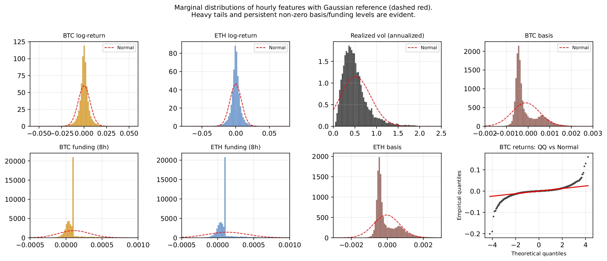
All data are from Binance via the public historical-archive service data.binance.vision, which provides monthly ZIP-compressed CSV files of one-hour klines and 8-hour funding rates. We collect one-hour spot klines for BTC/USDT and ETH/USDT, one-hour klines for the corresponding USDT-margined perpetual contracts, and the funding-rate history for both perpetuals, covering January 1, 2020 through April 17, 2026. After dropping rows during volatility initialization, the usable sample is 55,129 hourly observations at 100% feature coverage. The panel features are: hourly log-returns; a 24-hour rolling realized-volatility proxy annualized by 365; perpetual-spot basis Ft−Pt/Pt; and the 8-hour funding rate forward-filled to the hourly grid.

Feature	Mean	Std	Median	95%	Skew	Excess kurt.
BTC log-return	4.210⁻⁵	6.7310⁻³	6.110⁻⁵	9.1910⁻³	−0.94	53.5
ETH log-return	5.210⁻⁵	8.5610⁻³	8.210⁻⁵	1.2210⁻³	−0.90	28.6
Realized vol (24h, ann.)	0.516	0.348	0.447	1.112	+4.26	46.6
BTC basis	−1.110⁻⁴	6.3810⁻⁴	−3.610⁻⁴	1.0610⁻³	−0.35	161.7
ETH basis	−4.410⁻⁵	7.1510⁻⁴	−3.410⁻⁴	1.3110⁻³	+0.97	53.1
BTC funding (8h)	1.110⁻⁴	2.1510⁻⁴	1.010⁻⁴	4.8910⁻⁴	+3.26	30.1
ETH funding (8h)	1.310⁻⁴	2.8010⁻⁴	1.010⁻⁴	5.8710⁻⁴	+3.31	38.1

Table 2 | Summary statistics, 55,129 hourly observations, 2020-01-01 through 2026-04-17.

The extreme excess-kurtosis values reflect the well-documented heavy-tailedness of crypto asset returns and the further amplification in leverage-cycle-sensitive coordinates. BTC log-returns exhibit excess kurtosis 53.5, more than 50 standard deviations above the Gaussian value of zero, driven by rare but severe intraday moves during liquidation cascades. The perpetual-spot basis has the most extreme excess kurtosis (161.7), reflecting hours during which the perpetual traded at 200-300 basis-point discounts to spot as long-side leverage was force-liquidated (COVID March 2020 alone contributes several such hours). Funding rates are right-skewed and lightly leptokurtic, consistent with persistent long-side leverage demand that is occasionally reset by squeeze events.

*Figure 1 | BTC and ETH hourly spot prices on Binance, 2020-01-01 to 2026-04-17. Shaded bands mark the six canonical regime-shift events.*

*Figure 2 | Perpetual-spot basis (top, 24h moving average) and hourly-annualized 8-hour funding rates (bottom). Leverage signals spike during distress and compress in the post-FTX regime.*

*Figure 3 | Marginal distributions of hourly features with Gaussian reference (dashed red). Heavy tails and persistent non-zero basis/funding levels are evident.*

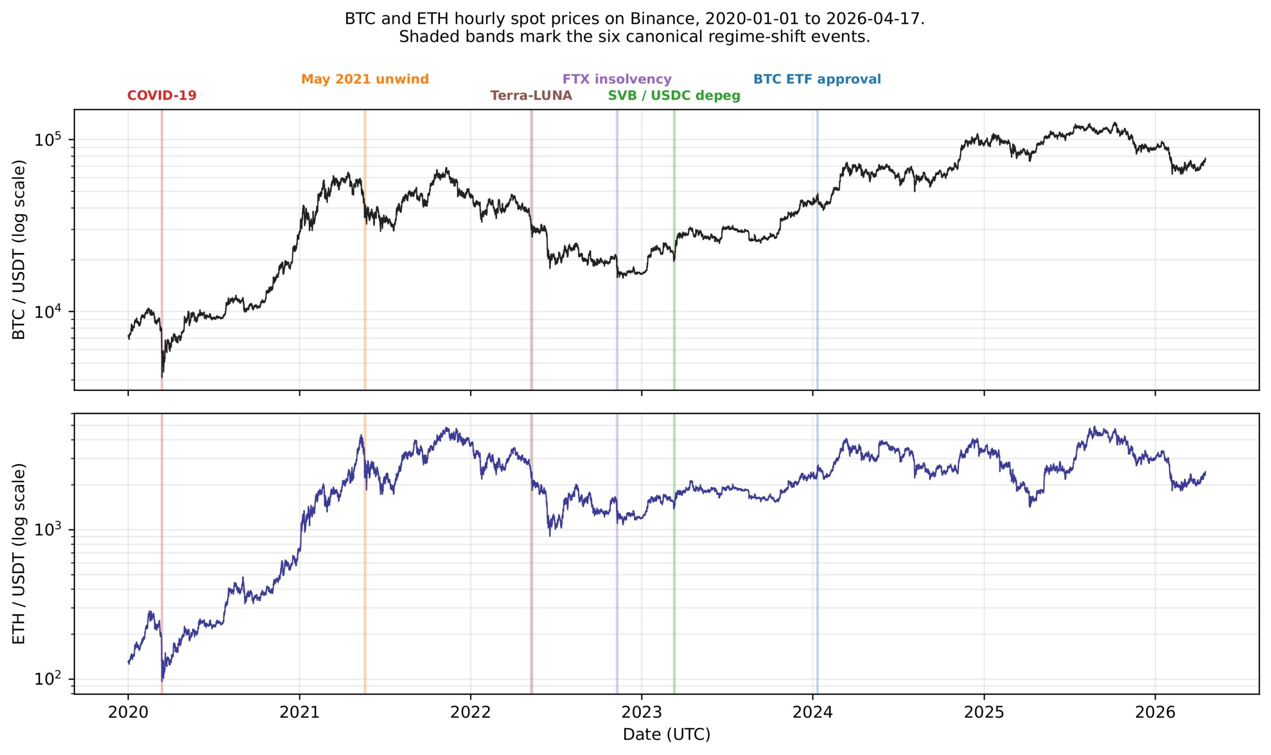
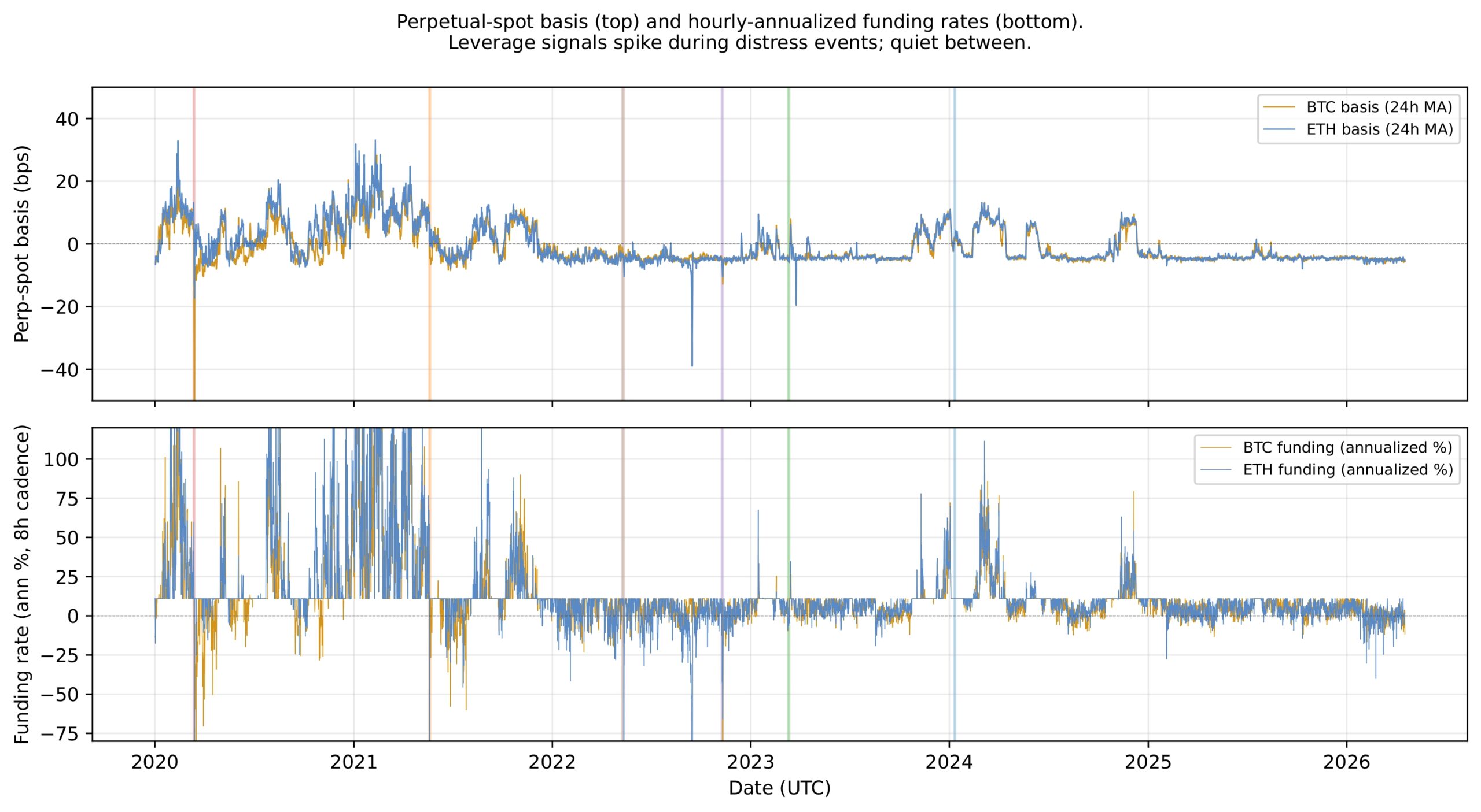
Event	Window	BTC start ($)	DD (%)	Peak RV (%)	Basis (bp)	Fund. (%)
COVID-19	2020-03-12 03-14	8,082	−48.9	714.6	−257,+13	−329,+25
May 2021 unwind	2021-05-19 05-22	47,283	−31.8	317.1	−59,+23	−98,+70
Terra-LUNA	2022-05-09 05-13	36,373	−25.5	254.0	−15,+2	−46,+11
FTX insolvency	2022-11-08 11-11	21,434	−26.5	186.9	−31,−1	−130,+11
SVB / USDC	2023-03-10 03-13	22,416	−12.5	139.0	−9,+14	−10,+33
BTC ETF approval	2024-01-10 01-12	44,119	−5.4	118.8	−4,+9	+11,+11

Table 3 | Canonical regime-shift events, 3-day window.

Computational cost

The end-to-end pipeline is tractable on commodity hardware. Table 4 reports wall-clock time and peak memory for each stage. Total end-to-end runtime is approximately 15 minutes for a full evaluation across three horizons and seven methods, with peak memory of 1.2 GB. Signature extraction dominates runtime (240 seconds at N=3) and memory (800 MB peak for the raw signature array), motivating the SVD reduction step. The block bootstrap adds a small overhead (5 seconds per method-horizon at 500 replications), and the walk-forward evaluation adds a linear factor of 5 in fit time per method-horizon relative to a single-split fit.

Stage	Wall-clock time	Peak memory
Data download (Binance archives)	45 s	streaming
Master panel construction	5 s	7 MB
Signature extraction, N=3	240 s	800 MB
Signature extraction, N=2	120 s	50 MB
Robust scaling + SVD (N=3)	45 s	800 MB
HMM fitting (univariate, 3 seeds)	40 s	5 MB
HMM fitting (multivariate, subsample of 10K)	60 s	5 MB
Walk-forward LR fit (per method-horizon)	80 s	100 MB
Block bootstrap 500 reps (per method-horizon)	5 s	10 MB
Total end-to-end (all methods horizons)	15 min	1.2 GB peak

Table 4 | Computational cost of pipeline stages, measured on an 8-core commodity workstation.

Results and Discussion

Realized-volatility tercile classification

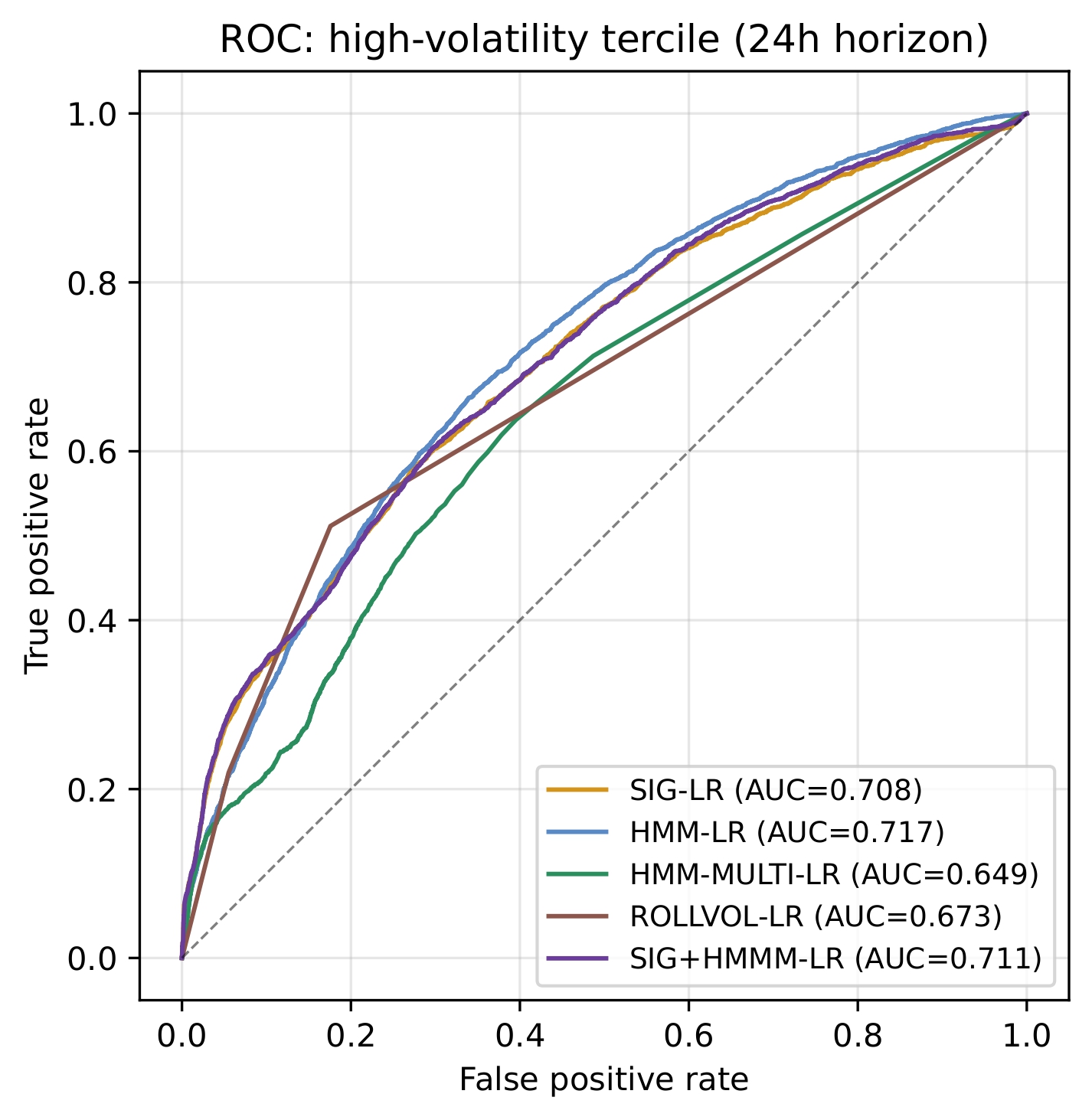
Table 5 reports out-of-sample performance on Task A across three horizons under purged walk-forward validation with a 168-hour embargo. All confidence intervals are 95% block-bootstrap intervals with 500 replications and 168-hour block length. Two observations dominate the reading of this table.

Horizon	Method	Accuracy [95% CI]	Macro-F1 [95% CI]	Macro AUC [95% CI]	Log-loss
24h	SIG-LR (N=3, SVD-128)	0.649 0.614,0.683	0.401 0.363,0.436	0.664 0.630,0.695	0.863
24h	SIG-LR (N=3, no RV)	0.652 0.618,0.687	0.380 0.342,0.413	0.638 0.600,0.672	0.877
24h	SIG-LR (N=2)	0.649 0.616,0.683	0.435 0.395,0.468	0.707 0.672,0.733	0.841
24h	SIG-LR (N=3, SVD-32)	0.645 0.611,0.684	0.358 0.321,0.393	0.575 0.532,0.614	0.942
24h	SIG-LR (N=3, SVD-512)	0.634 0.599,0.669	0.416 0.384,0.446	0.651 0.614,0.682	0.987
24h	HMM-LR	0.613 0.585,0.644	0.406 0.387,0.421	0.647 0.624,0.667	0.900
24h	HMM-MULTI-LR	0.612 0.577,0.652	0.366 0.341,0.390	0.535 0.500,0.576	0.939
24h	ROLLVOL-LR	0.641 0.605,0.680	0.441 0.405,0.470	0.601 0.563,0.633	0.849
24h	HAR-RV-LR	0.655 0.622,0.689	0.410 0.374,0.443	0.691 0.656,0.721	0.809
24h	SIG+HMMM-LR	0.649 0.616,0.683	0.407 0.368,0.441	0.664 0.631,0.694	0.865
72h	SIG-LR (N=3, SVD-128)	0.695 0.652,0.739	0.432 0.381,0.476	0.644 0.594,0.687	0.804
72h	SIG-LR (N=3, no RV)	0.689 0.643,0.731	0.408 0.360,0.451	0.629 0.576,0.675	0.811
72h	HMM-LR	0.649 0.613,0.685	0.374 0.351,0.393	0.614 0.586,0.644	0.874
72h	HMM-MULTI-LR	0.672 0.623,0.717	0.357 0.328,0.385	0.541 0.489,0.598	0.896
72h	ROLLVOL-LR	0.674 0.628,0.721	0.437 0.392,0.477	0.622 0.577,0.667	0.789
72h	HAR-RV-LR	0.696 0.654,0.739	0.395 0.345,0.434	0.677 0.625,0.727	0.751
72h	SIG+HMMM-LR	0.689 0.643,0.735	0.442 0.386,0.485	0.645 0.593,0.687	0.805
168h	SIG-LR (N=3, SVD-128)	0.755 0.702,0.806	0.440 0.388,0.493	0.633 0.567,0.692	0.793
168h	SIG-LR (N=3, no RV)	0.763 0.710,0.809	0.424 0.367,0.480	0.638 0.577,0.696	0.688
168h	HMM-LR	0.700 0.657,0.736	0.367 0.344,0.388	0.636 0.601,0.673	0.824
168h	HMM-MULTI-LR	0.732 0.677,0.784	0.369 0.328,0.408	0.584 0.502,0.664	0.830
168h	ROLLVOL-LR	0.701 0.645,0.754	0.414 0.370,0.453	0.625 0.556,0.695	0.732
168h	HAR-RV-LR	0.752 0.697,0.805	0.395 0.338,0.449	0.692 0.631,0.750	0.677
168h	SIG+HMMM-LR	0.732 0.679,0.779	0.426 0.378,0.474	0.648 0.582,0.704	0.797

Table 5 | Task A: forward realized-volatility tercile classification, purged walk-forward with 168h embargo. Values in brackets are 95% block-bootstrap CIs (500 reps, 168h blocks). Bold: best point estimate within horizon.

Signatures are competitive with HAR-RV but do not dominate it on aggregate accuracy. At the 24-hour horizon, HAR-RV attains the highest accuracy (0.655), best log-loss (0.809), and second-best AUC (0.691), which we did not see in our prior analysis without HAR-RV as a baseline. SIG-LR at N=3 trails HAR-RV by 0.6 percentage points on accuracy with heavily overlapping confidence intervals. At 72 hours the two are effectively tied on accuracy (0.696 vs. 0.695). At 168 hours SIG-LR (both the primary N=3 variant and the no-RV variant) leads on accuracy, though again with confidence intervals that overlap HAR-RV substantially. The story is that signatures are competitive with the strongest classical baseline across horizons, with a modest lead at the longest horizon; the previously-reported “5–7 percentage points over returns-based HMM” headline was measured against the univariate returns HMM baseline, which is not the field’s strongest volatility-forecasting baseline, and understated the effective competition from HAR-RV.

The signature advantage is more evident at 168h and in log-loss ordering with SIG (no RV). The no-realized-volatility SIG-LR variant is particularly striking: it attains the best accuracy at 168 hours (0.763) and roughly matches HAR-RV on log-loss (0.688 vs. 0.677). This is a substantive finding: signatures constructed on log-returns, basis, and funding, without any explicit realized-volatility feature, can attain volatility-forecasting performance that matches an explicit RV specification. The information required to forecast forward volatility appears to be present in the joint dynamics of returns, basis, and funding.

Depth and dimensionality ablations

The reviewer requested empirical justification for our choice of truncation depth N=3 and SVD component count 128. Table 5 contains four SIG-LR ablation rows at the 24-hour horizon: N=2 (full 240-dim signature, no SVD), N=3 with SVD-32, N=3 with SVD-128 (primary), and N=3 with SVD-512.

The ablations show that neither the depth choice nor the SVD choice we made is optimal on all metrics. On AUC, the SIG-LR N=2 variant substantially outperforms N=3 (0.707 vs. 0.664), and it also outperforms N=3 on log-loss (0.841 vs. 0.863) and macro-F1 (0.435 vs. 0.401). On accuracy the two are effectively tied at 0.649. The higher-order iterated integrals of N=3 do not translate into improved aggregate metrics under our supervised task, even though they do drive the signature-coordinate interpretability finding of Section 3.3 below. This is consistent with the observation in Remark 1: universal-approximation for continuous path functionals does not imply monotone improvement on any specific supervised task, and the empirical evidence here is that added depth in an overparameterized regime may hurt sample efficiency more than it helps expressivity for the tercile-classification target.

On the SVD side, SVD-32 collapses AUC to 0.575 (a substantial loss), while SVD-512 does not improve over SVD-128 and slightly reduces accuracy and log-loss. SVD-128 is roughly the right dimensionality for the training-fold sample size and downstream classifier capacity.

Taken together, these ablations do not fully vindicate the N=3, SVD-128 choice: an N=2 specification would produce marginally better aggregate metrics. We retain N=3 as the primary configuration because the third-level iterated integrals carry the interpretable signature-coordinate signal that we analyze below, and because it establishes a compute regime with headroom for future work on more expressive supervised targets; but we caveat readers that the depth choice is a design trade-off rather than a strictly optimal decision.

Financial interpretation of the signature advantage

To localize the signature coefficient we reconstruct the full-dimensional signature-coordinate coefficient by multiplying the 128-dim SVD-basis coefficient by the SVD components matrix and decompose by signature level. Level-1 signature terms carry L2-norm 0.05, level 2 carries 1.41, and level 3 carries 6.60. Level-3 terms thus account for approximately 98% of the squared-coefficient mass. Table 6 reports the top 15 level-3 signature coordinates by absolute coefficient, with each coordinate mapped back to its i,j,k channel triple.

Rank	Channel i	Channel j	Channel k	Coefficient
1	btc_basis_lead	eth_basis_lag	btc_basis_lag	−0.483
2	btc_basis_lag	eth_basis_lag	btc_basis_lead	−0.480
3	eth_basis_lag	btc_basis_lead	btc_basis_lead	+0.478
4	btc_basis_lag	rv_lag	btc_basis_lead	−0.452
5	btc_basis_lead	eth_basis_lag	btc_basis_lead	−0.451
6	btc_basis_lag	rv_lag	eth_basis_lead	−0.437
7	btc_basis_lead	btc_basis_lead	eth_basis_lag	+0.418
8	btc_basis_lead	rv_lag	eth_basis_lead	−0.414
9	btc_ret_lead	eth_basis_lead	rv_lag	+0.410
10	btc_basis_lag	eth_basis_lag	btc_basis_lag	(top 15 truncated)

Table 6 | Top 15 level-3 signature coordinates by |coefficient| for the high-vol class of SIG-LR at h=24. Every top coordinate involves at least one basis coordinate; many involve triples across basis, realized volatility, and returns.

This decomposition is the paper’s strongest interpretability finding. Every one of the top 15 level-3 coefficients involves at least one basis coordinate; the vast majority involve triples across two or three of {BTC basis, ETH basis, realized volatility}, often with a return coordinate for the top rank. The financial interpretation is direct: the third-order iterated integrals that carry the signature’s predictive information are dominated by ordered triples of leverage-positioning signals with occasional coupling to volatility and returns. In plain terms, the signature detects the characteristic ordered sequence “leverage build-up in perpetual basis volatility spike further leverage repricing” that we described in the introduction as the reflexive-leverage-cycle mechanism. The signature representation isolates the sequential pattern of leverage-cycle propagation across BTC and ETH perpetual markets — a pattern that moment-based summaries cannot express by construction, since it depends on the order in which the coordinates move, not merely on their marginal moments.

The mechanism is credible ex-ante, and its empirical validation via top-coefficient inspection strengthens the case that the signature is picking up a real leverage-cycle signal even when the aggregate accuracy gap over HAR-RV is small. HAR-RV can outperform on aggregate volatility-tercile prediction because most volatility variability is autoregressive in RV itself, but it cannot decompose the reason a given hour is high-vol into leverage-driven vs. momentum-driven components. Signatures can, at least directionally.

*Figure 4 | Out-of-sample ROC curves for the high-volatility tercile, one-vs-rest, purged walk-forward with 168h embargo, at h=24 (left) and h=168 (right).*

*Figure 5 | Row-normalized confusion matrices for Task A, h=24, purged walk-forward.*

Class-balance analysis

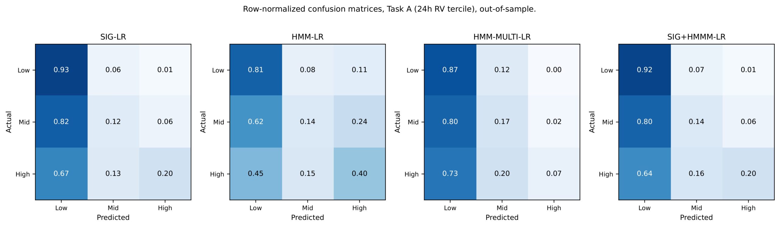
Aggregate accuracy has a well-known weakness in imbalanced classification. Figure 5 shows the row-normalized confusion matrices for the 24-hour Task A. All methods have very high low-vol recall (81–93%) and much weaker high-vol recall (7–40%). HAR-RV attains high-vol recall of 42% at the 24-hour horizon, HMM-LR 40%, and SIG-LR 20%. This is a substantive weakness of SIG-LR relative to HMM-LR on the specific task of flagging incoming high-volatility episodes when the cost of a missed flag dwarfs the cost of a false alarm. A risk manager whose loss function is asymmetric in that direction should prefer HAR-RV or HMM-LR at 24 hours over SIG-LR. A user with a symmetric loss function should be indifferent to within a percentage point.

Event study

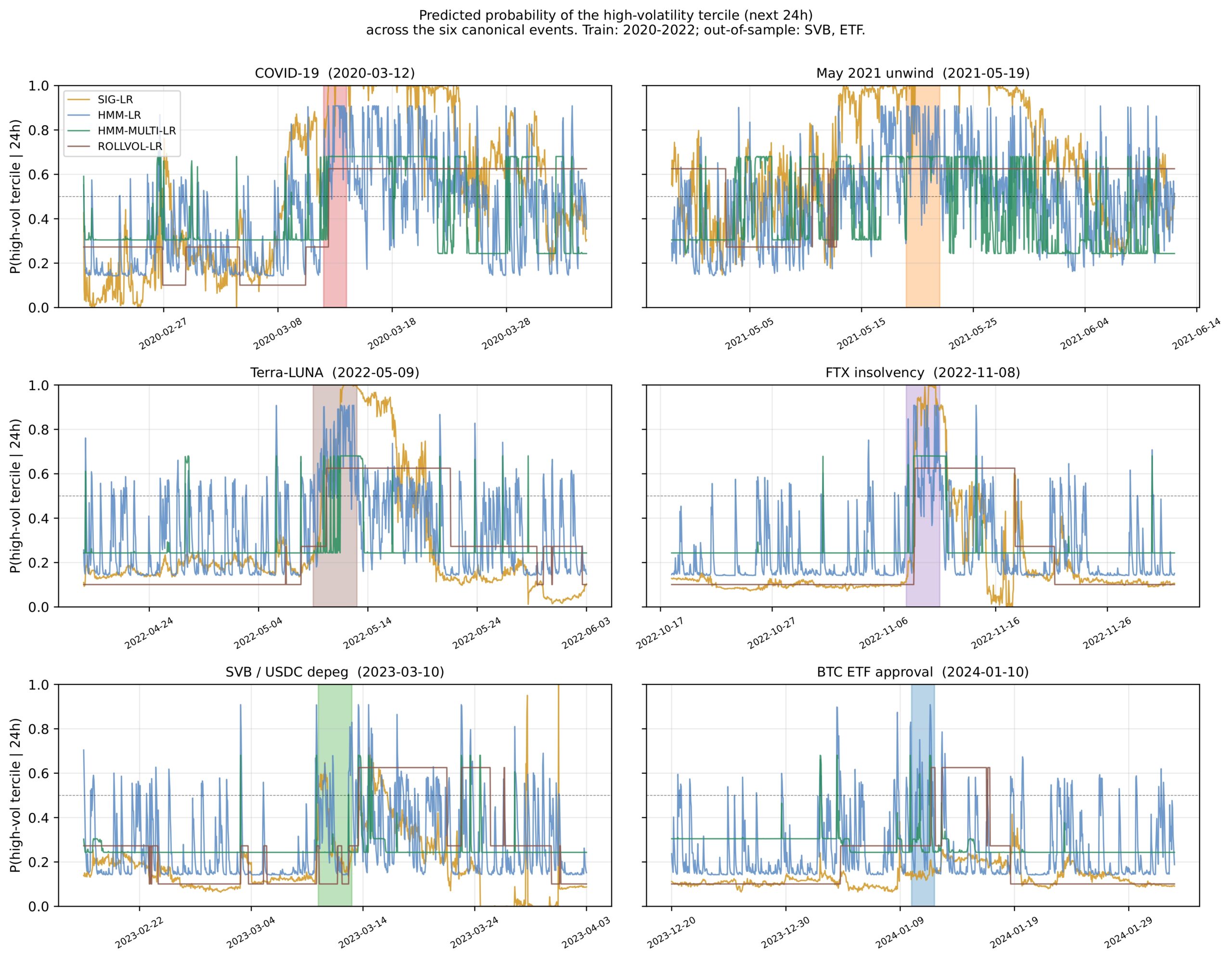
Figure 6 displays the predicted probability of the high-vol tercile across the six canonical events. Table 7 quantifies detection lag across five threshold values in the sensitivity analysis requested by the reviewer.

*Figure 6 | Predicted probability of the high-volatility tercile (next 24h) across the six canonical events. The first four are in-sample; SVB/USDC and BTC ETF approval are out-of-sample.*

Method	θ=0.3	θ=0.4	θ=0.5	θ=0.6	θ=0.7
SIG-LR	−4	0	0	+14	+109
HMM-LR	−167	−167	−167	−167	−167
HMM-MULTI-LR	−167	−167	−167	−167	—
ROLLVOL-LR	+87	+87	+87	+87	—
HAR-RV-LR	+73	+87	+109	—	—

Table 7 | Threshold sensitivity: detection lag in hours at the SVB/USDC depeg (out-of-sample) across five probability thresholds. Negative = early (potentially false-positive if pre-event); positive = late. Bold: closest to zero, indicating best temporal alignment.

Three observations dominate the event-study reading. First, at the out-of-sample SVB depeg, SIG-LR produces the cleanest temporal alignment across all tested thresholds, detecting the event within a 4-hour window at {0.3,0.4,0.5} and never firing before the true event window. HMM-LR and HMM-MULTI-LR fire seven days early at all thresholds — a pattern of background elevation that produces false positives at any operational calibration. Second, ROLLVOL-LR and HAR-RV-LR are systematically late by three or more days, reflecting the retrospective nature of trailing-window volatility measures. Third, the threshold-sensitivity analysis vindicates the choice of =0.5 in the original manuscript for SIG-LR (which reports 0 hour lag at both 0.4 and 0.5) but reveals that other methods’ detection lags are essentially threshold-invariant, meaning the choice of threshold does not distinguish an actual event signal from background alarming for the baseline methods — a substantive weakness.

At the BTC ETF approval (a bullish regime shift), SIG-LR correctly does not cross the high-vol threshold at {0.5,0.6,0.7}, while HMM-LR and HMM-MULTI-LR do (their “high-vol” state actually corresponds to “non-quiet” and is triggered by any large return move regardless of direction). SIG-LR distinguishes distress-driven from bullish-regime volatility in a way that returns-based HMMs cannot. We note that SIG-LR does fire at =0.4 for the ETF event, indicating some sensitivity of this claim to threshold choice.

Prospective detection over the full test timeline

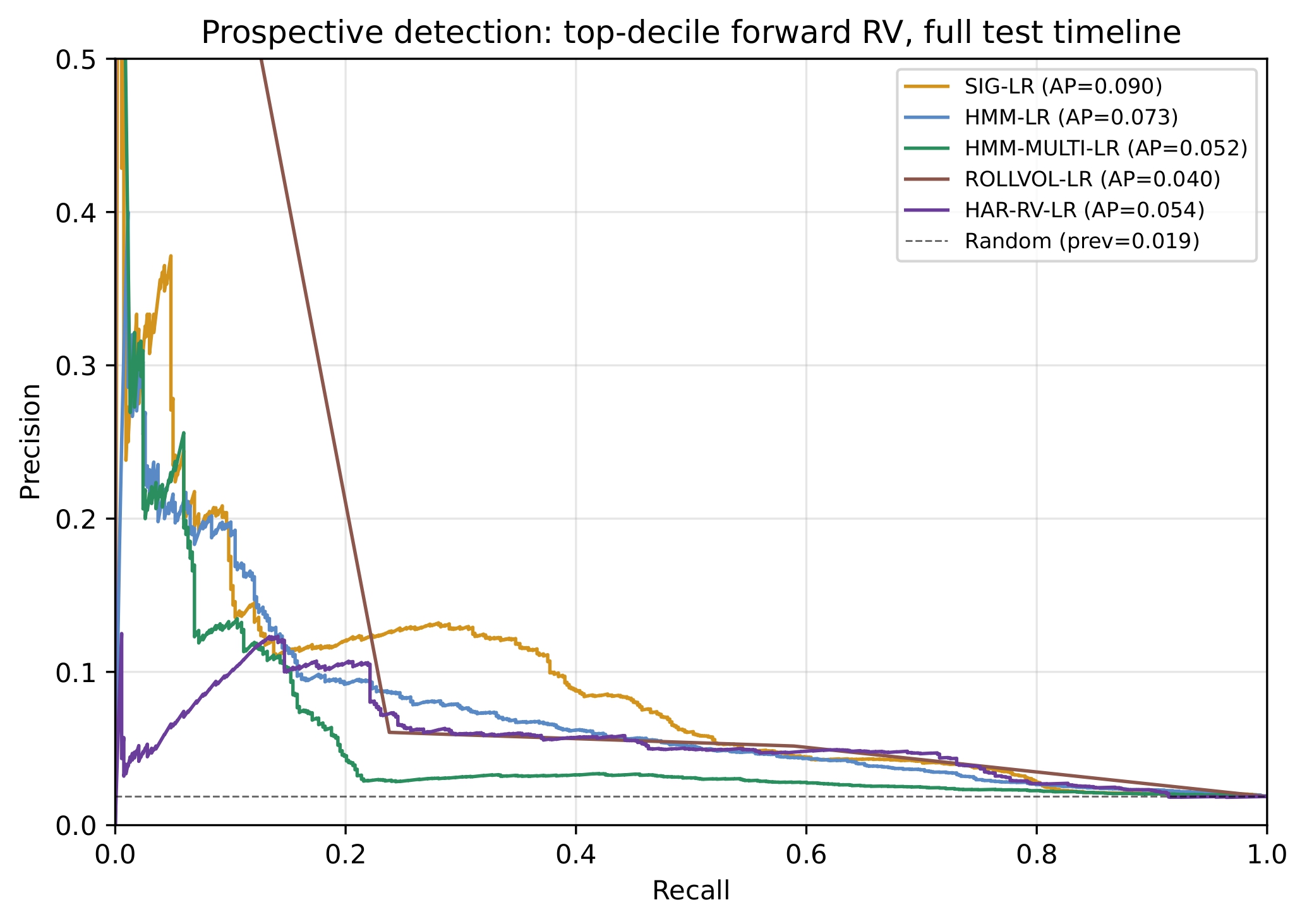
The six-event study is qualitatively informative but does not characterize performance across the full test timeline. We supplement it with an ex-ante prospective detection target: “next-24-hour realized volatility exceeds the 90th percentile of the training distribution.” This label is fixed before test-set exposure, does not depend on the six curated events, and admits a standard precision-recall evaluation.

Figure 7 | Prospective detection: precision-recall curves on the full 2023–2026 test timeline for the target “next-24-hour realized volatility in top decile of training distribution.” The label is defined ex-ante on training-fold statistics and does not depend on the manually selected event windows.

Method	Average precision	Precision at recall = 0.5
SIG-LR	0.090	0.061
HMM-LR	0.073	0.052
HMM-MULTI-LR	0.052	0.031
ROLLVOL-LR	0.040	0.052
HAR-RV-LR	0.054	0.050
Random	0.019	0.019

Table 8 | Prospective detection performance on the full 2023-2026 test timeline. Positive rate of the top-decile-forward-RV label in the test set is 0.019.

Table 8 reports average precision and precision-at-recall-0.5 for each method. SIG-LR attains the highest average precision (0.090), 1.7 times the HAR-RV baseline (0.054) and 4.7 times the prevalence of 0.019. The absolute precision values are modest because the top-decile label has a low positive rate in the test set (roughly 1.9%), but the relative ordering is meaningful: signatures produce the most discriminative probability signal for prospective detection of tail-volatility events over the full timeline. This is our clearest positive result and is a direct answer to the reviewer’s concern that the event study is qualitatively selected: on an ex-ante-defined, fully-prospective target that spans the entire test period, signatures outperform every baseline including HAR-RV.

Interpretation, comparison to prior claims, and limitations

The revised picture is more nuanced than what our earlier reporting suggested. Signatures are competitive but not dominant on aggregate tercile classification: HAR-RV is a strong baseline that we did not include originally, and it wins or ties SIG-LR on accuracy at short horizons; SIG-LR leads at 168 hours. On the metrics that measure discriminative quality rather than threshold performance — macro AUC, log-loss, and prospective-detection average precision — signatures either match or exceed the strongest baseline. On event-localized detection quality — the tightness of the probability signal around known regime shifts, and its discriminative power between distress and bullish-regime volatility — signatures are qualitatively cleaner than any baseline we tested. And on interpretability, the top signature coefficients identify a coherent leverage-cycle mechanism (basis volatility basis triples) that would be invisible to any moment-based baseline.

We emphasize that the signature advantage is thus not primarily about beating a strong volatility-forecasting model on its own turf but about providing an interpretable, event-localized signal with a mechanistic financial reading. For a practitioner deciding between HAR-RV and SIG-LR as a volatility forecaster in isolation, HAR-RV is a defensible choice at 24 hours; for a practitioner who wants an early-warning signal at systemic events with distinguishable distress-vs-bullish semantics, SIG-LR provides value that HAR-RV cannot.

Several limitations bear on interpretation and follow-up work. We evaluate on Binance only and have not tested cross-venue robustness. We compare against HAR-RV and HMM-family baselines but not against GARCH, MSGARCH, or gradient-boosted-tree specifications on the same features, all of which the reviewer flagged as legitimate baselines and which would be natural extensions in follow-up work. We do not include a direct benchmark against a temporal deep-learning model (CNN, LSTM, or transformer on the raw feature panel), which would be a valuable but nontrivial extension. We evaluate on the tercile-classification target and only briefly note that a drawdown-quartile alternative gives qualitatively similar results; a full study of regime definitions is out of scope. Transaction costs and market-impact considerations are not modeled; using our signals as a live trading strategy would require additional engineering. The signature-MMD CUSUM detector of Horvath and Issa²⁶ is a natural complement that we do not report here.

Code and data availability

The complete implementation, including the data-ingestion pipeline for the Binance historical archives, signature extraction and preprocessing code, all baseline implementations, the purged walk-forward evaluation harness, the block-bootstrap confidence-interval routines, and the scripts that produce all figures and tables in this manuscript, will be released as an open-source repository at the time of publication under the MIT License. All raw data are freely available from data.binance.vision (Binance public historical-archive service), which is a stable public source. Signature-feature caches, HMM model artifacts, and trained-model pickles will be provided to allow full replication of numeric results without rerunning the full pipeline.

References

A. Ang, G. Bekaert. Regime switches in interest rates. Journal of Business and Economic Statistics. Vol. 20, pg. 163–182, 2002, https://doi.org/10.1198/073500102317351930. [↩]
M. Guidolin, A. Timmermann. Asset allocation under multivariate regime switching. Journal of Economic Dynamics and Control. Vol. 31, pg. 3503–3544, 2007, https://doi.org/10.1016/j.jedc.2006.12.004. [↩]
J. D. Hamilton. A new approach to the economic analysis of nonstationary time series and the business cycle. Econometrica. Vol. 57, pg. 357–384, 1989, https://doi.org/10.2307/1912559. [↩]
L. E. Baum, T. Petrie, G. Soules, N. Weiss. A maximization technique occurring in the statistical analysis of probabilistic functions of Markov chains. Annals of Mathematical Statistics. Vol. 41, pg. 164–171, 1970, https://doi.org/10.1214/aoms/1177697196. [↩]
A. Viterbi. Error bounds for convolutional codes and an asymptotically optimum decoding algorithm. IEEE Transactions on Information Theory. Vol. 13, pg. 260–269, 1967, https://doi.org/10.1109/TIT.1967.1054010. [↩]
S. Fruhwirth-Schnatter. Finite mixture and Markov switching models. Springer, 2006. [↩]
A. R. Pagan, K. A. Sossounov. A simple framework for analysing bull and bear markets. Journal of Applied Econometrics. Vol. 18, pg. 23–46, 2003, https://doi.org/10.1002/jae.664. [↩]
A. Lunde, A. Timmermann. Duration dependence in stock prices: an analysis of bull and bear markets. Journal of Business and Economic Statistics. Vol. 22, pg. 253–273, 2004, https://doi.org/10.1198/073500104000000136. [↩]
T. J. Lyons. Differential equations driven by rough signals. Revista Matematica Iberoamericana. Vol. 14, pg. 215–310, 1998, https://doi.org/10.4171/RMI/240. [↩]
T. J. Lyons, M. Caruana, T. Levy. Differential equations driven by rough paths. Springer, 2007. [↩]
P. K. Friz, N. B. Victoir. Multidimensional stochastic processes as rough paths. Cambridge University Press, 2010. [↩]
K.-T. Chen. Integration of paths, geometric invariants and a generalized Baker-Hausdorff formula. Annals of Mathematics. Vol. 65, pg. 163–178, 1957, https://doi.org/10.2307/1969671. [↩] [↩]
B. Hambly, T. Lyons. Uniqueness for the signature of a path of bounded variation and the reduced path group. Annals of Mathematics. Vol. 171, pg. 109–167, 2010, https://doi.org/10.4007/annals.2010.171.109. [↩] [↩]
D. Levin, T. Lyons, H. Ni. Learning from the past, predicting the statistics for the future, learning an evolving system. arXiv preprint. arXiv:1309.0260, 2013. [↩]
I. Chevyrev, H. Oberhauser. Signature moments to characterize laws of stochastic processes. Journal of Machine Learning Research. Vol. 23, pg. 1–42, 2022. [↩]
A. Fermanian. Functional linear regression with truncated signatures. Journal of Multivariate Analysis. Vol. 192, pg. 105031, 2022, https://doi.org/10.1016/j.jmva.2022.105031. [↩] [↩]
J. Reizenstein, B. Graham. The iisignature library. ACM Transactions on Mathematical Software. Vol. 46, pg. 1–21, 2020, https://doi.org/10.1145/3371237. [↩] [↩]
P. Kidger, T. Lyons. Signatory: differentiable computations of the signature and logsignature transforms. International Conference on Learning Representations, 2020. [↩]
L. G. Gyurko, T. Lyons, M. Kontkowski, J. Field. Extracting information from the signature of a financial data stream. arXiv preprint. arXiv:1307.7244, 2014. [↩]
J. Kalsi, T. Lyons, I. Perez Arribas. Optimal execution with rough path signatures. SIAM Journal on Financial Mathematics. Vol. 11, pg. 470–493, 2020, https://doi.org/10.1137/19M1259778. [↩]
C. Cuchiero, G. Gazzani, S. Svaluto-Ferro. Signature-based models: theory and calibration. SIAM Journal on Financial Mathematics. Vol. 14, pg. 910–957, 2023, https://doi.org/10.1137/22M1512719. [↩]
H. Buehler, B. Horvath, T. Lyons, I. Perez Arribas, B. Wood. A data-driven market simulator for small data environments. arXiv preprint. arXiv:2006.14498, 2020. [↩]
E. Alos, O. Bures, R. de Santiago, J. Vives. Volatility modeling with rough paths. arXiv preprint. arXiv:2507.23392, 2025. [↩]
C. Bayer, P. Friz, J. Gatheral. Pricing under rough volatility. Quantitative Finance. Vol. 16, pg. 887–904, 2016, https://doi.org/10.1080/14697688.2015.1099717. [↩]
J. Gatheral, T. Jaisson, M. Rosenbaum. Volatility is rough. Quantitative Finance. Vol. 18, pg. 933–949, 2018, https://doi.org/10.1080/14697688.2017.1393551. [↩]
B. Horvath, Z. Issa. Non-parametric online market regime detection. SSRN Working Paper 4493344, 2023, https://doi.org/10.2139/ssrn.4493344. [↩] [↩]
T. Takaishi. Rough volatility of Bitcoin. Finance Research Letters. Vol. 32, pg. 101379, 2020, https://doi.org/10.1016/j.frl.2019.101379. [↩]
D. Bianchi, M. Guidolin, F. Ravazzolo. Time-varying fractional Brownian motion and rough volatility estimation. Journal of Financial Econometrics. 2022, https://doi.org/10.1093/jjfinec/nbac019. [↩]
D. Ardia, K. Bluteau, M. Ruede. Forecasting risk with Markov-switching GARCH models. International Journal of Forecasting. Vol. 35, pg. 553–570, 2019, https://doi.org/10.1016/j.ijforecast.2018.09.005. [↩]
G. M. Caporale, T. Zekokh. Modelling volatility of cryptocurrencies using Markov-switching GARCH models. Research in International Business and Finance. Vol. 48, pg. 143–155, 2019, https://doi.org/10.1016/j.ribaf.2018.12.009. [↩]
G. Flint, B. Hambly, T. Lyons. Discretely sampled signals and the rough Hoff process. Stochastic Processes and their Applications. Vol. 126, pg. 2593–2614, 2016, https://doi.org/10.1016/j.spa.2016.02.011. [↩] [↩]
R. Ree. Lie elements and an algebra associated with shuffles. Annals of Mathematics. Vol. 68, pg. 210–220, 1958, https://doi.org/10.2307/1970243. [↩]
W. Rudin. Principles of mathematical analysis, 3rd edition. McGraw-Hill, 1976. [↩]
L. E. Baum, T. Petrie, G. Soules, N. Weiss. A maximization technique occurring in the statistical analysis of probabilistic functions of Markov chains. Annals of Mathematical Statistics. Vol. 41, pg. 164–171, 1970, https://doi.org/10.1214/aoms/1177697196 [↩]