Representing Cinematic Style with Neural Style Transfer: A Case Study of Films by Wes Anderson and Tim Burton

Abstract

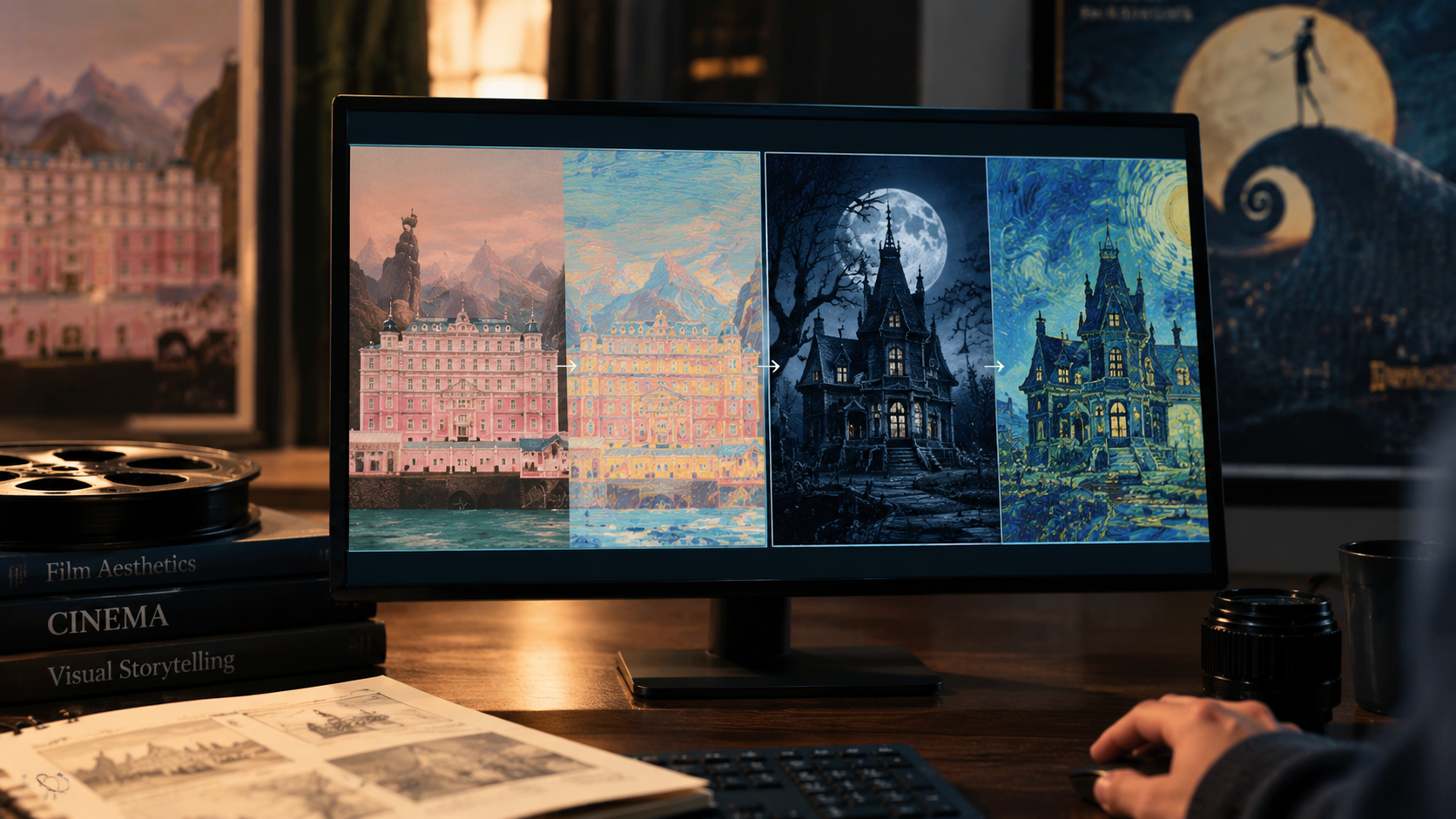
This paper investigated how Neural Style Transfer (NST) can be adapted to render images in cinematic styles, focusing on lighting and color distribution featured in movies by Wes Anderson and Tim Burton. Cinematic style lies between the domain of non-photorealistic and photorealistic rendering, as the live-action movie frames can feature both elements from real-life scenarios and artistic choices. In this study, using a self-curated film-based style dataset—in which each cinematic style was represented by 14 reference frames from a single film—I implemented a multi-style transfer framework using Conditional Instance Normalization. Two experiments were conducted: Experiment 1 used a single-frame style representation, whereas Experiment 2 used an average Gram-matrix representation derived from all 14 frames belonging to each style. To evaluate how well the two methods capture cinematic color and lighting distribution, normalized one-dimensional color histograms of the L, A, and B channels in the LAB color space were extracted from the stylized outputs and compared with those of the corresponding reference frame collections. The results showed that both single-frame and average Gram-matrix representations enabled the NST model to transfer measurable color and lighting distributions. However, the average Gram-matrix representation generally produced outputs closer to the reference-frame collections. Performance varied across styles, input images, and independent training runs. Because this study was rather small and exploratory, its findings should be interpreted cautiously and cannot be generalized to other directors, films, model architectures, or reference-frame selection pipelines without further investigation. 

Keywords: Neural Style Transfer, Convolutional Neural Network, Conditional Instance Normalization (CIN), Cinematic Style

Introduction

Cinematography is the visual language of storytelling in cinema. From pastel-hued and symmetrical frames in The Grand Budapest Hotel to the neon-drenched landscapes of The Matrix, cinematography serves not only as the filmmaker’s language but also as a visual metaphor to convey emotion and social commentary. However, translating such complex and varied visual languages onto static images has often remained a challenge for traditional image editing.

The emergence of Neural Style Transfer (NST) presented promising avenues for translating cinematic storytelling into static images. NST, a branch of non-photorealistic rendering, was shaped by the landmark paper “Image Style Transfer using Convolutional Neural Network” by Gatys and colleagues¹. They proposed an iterative optimization method based on the pretrained VGG-19 network². This approach produced high-quality stylized images with arbitrary input images but demanded significant computational resources, requiring hundreds to thousands of forward-backward passes through the VGG-19 network per image. Many works had since then attempted to accelerate this costly optimization method. Johnson et al.³ trained a feed-forward convolutional neural network (CNN) that had been previously adapted for image transformation tasks. However, a major limitation of the feed-forward network was that it is tied to only one style. For style transfer with multiple styles, separate networks would have to be trained for each style being modelled, which had high computational requirements. To address this, several CNN-based approaches were developed by Dumoulin et al.⁴, Chen et al.⁵, Li et al.⁶, and Zhang and Dana⁷. Notwithstanding, those works modelled each artistic style using a single representative reference style image. Studies like Ikuta et al.⁸ and Sanakoyeu et al.⁹ were built on the observation that an artistic style cannot be sufficiently captured through the stylistic features of a single work, thereby proposing multi-image style representation on collections of style-associated images.

There have been limited studies focusing on reproducing cinematic looks onto images, which occupy a unique middle ground between non-photorealistic and photorealistic rendering. While many live-action movie frames are realistic, their intentional use of color distribution, composition, and cinematography reflects artistic choices. A recent study by Zabaleta and Bertalmío¹⁰ presented a method that automatically transfers cinematic looks from a reference image, in terms of tone, color palette, and contrast, to the source RAW image, but it primarily lies in the domain of photorealistic style transfer. Therefore, there is a lack of studies addressing whether CNN-based multi-style transfer frameworks can be applied to cinematic styles and transfer them to images. 

This paper aimed to bridge this gap. Drawing on the multi-style framework of Dumoulin et al.⁴ and studies that propose multi-image style representation, such as Ikuta et al.⁸ and Sanakoyeu et al.⁹, I explored the possibility of using Conditional Instance Normalization (CIN) and Gram-matrix averaging to capture cinematic stylizations associated with Wes Anderson’s and Tim Burton’s filmography. In this study, cinematic style was considered a multifaceted construct reflected in still frames through a combination of color and lighting distributions. Therefore, Wes Anderson and Tim Burton were selected as two case studies because their films exhibited distinctive cinematic visuals.

In this study, I implemented two experiments: the first utilized a single representative style image for each style being modelled, whereas the second employed aggregated Gram-based representations computed from each style’s entire corpus of cinematic frames. Both of the experiments were tested on a film-based style dataset to see which one better captured the cinematic styles in terms of lighting and color distribution. Thus, my research aimed to answer the following questions:

RQ1: How well does the proposed CIN-based framework reproduce the color and lighting distributions associated with selected cinematic styles?

RQ2: To what extent do single-frame and average Gram-matrix style representations differ in their transfer of color and lighting distributions? 

It is also important to distinguish this research’s objective from photorealistic style transfer, exemplified by the approach proposed by Luan et al.¹¹ to preserve photorealism. While the latter focuses on meticulous content preservation, this study chose to focus on the artistic style transfer effects on the images.

Related Works

Multi-style transfer: Several CNN-based multi-style transfer frameworks had attempted to encode multiple artistic styles into an embedding space. For instance, Dumoulin et al.⁴ discovered that multi-style transfer can be sufficiently achieved by scaling and shifting parameters after normalization to each specific style. Therefore, the study introduced Conditional Instance Normalization (CIN) into a feed-forward image transformation network—similar to the architecture by Johnson et al.³—which normalized and transformed the content feature maps using a pair of style-specific parameters for each style being modelled. Other approaches explored alternative architectures: StyleBank⁵ utilized multiple mid-level convolutional filter banks to capture individual styles whereas Li et al.⁶, treated each bit in the selection unit as a distinct style. While these methods embedded styles with one-dimensional representations, Zhang and Dana⁷ introduced a CoMatch layer that took in the content feature maps, Gram matrices of the style image at multiple scales, and a learnable weight matrix W to approximate a stylized solution. 

Multi-image style representation: Recognizing that most CNN-based multi-style transfer approaches treated each reference style image as a distinct artistic style, there had been studies aiming to capture dominant style features across a collection of style images. One of the first studies to introduce the idea of aggregating Gram matrices across multiple styles was conducted by Ikuta et al.⁸. The study showed that the normalized Gram matrix of a concatenated image is approximately equal to the weighted linear combination of the normalized Gram matrices of its constituent images. Building on the assumption that any concatenation of reference images drawn in the same style also belongs to that style, the authors defined a style space in which weighted linear combinations of the reference images’ normalized Gram matrices also represented texture features of the target style. The model then learned an optimal blending ratio for these Gram matrices to estimate an appropriate texture for the content image before performing style transfer. Another study that briefly discussed Gram-matrix aggregation is the work by Sanakoyeu et al.⁹. Adopting the art historical standpoint that “style as an expression of a collective spirit”, the study argued that using a single artwork might not be enough for an artistic style to be sufficiently learnt. They found that averaging was the best Gram-matrix aggregation strategy, but combining Gram matrices from multiple images could sometimes cause over smoothing and unsatisfactory results.

Film-style transfer: To the best of my knowledge, “Photorealistic style transfer for cinema shoots” by Zabaleta and Bertalmío¹⁰ was the closest work to my study. However, it primarily focused on photorealistic style transfer. The study aimed to emulate the cinematic look present in a reference image, such as a still from an existing movie, by introducing a method that automatically transferred the style to the source RAW image in real-time. Their method could effectively generate the photorealistic results that were free of artifacts in real-time with low computational complexity in three consecutive but separable operations: Luminance transfer, Color transfer, and Local contrast.

Wes Anderson: An American director, screenwriter, and producer, Wes Anderson was known for his unique and consistent visual language throughout his filmography¹². His films typically featured the symmetrical, planimetric, and frontal shots¹³, vibrant and colorful production design¹². Color was also one of the stylistic elements in Wes Anderson’s visual storytelling¹⁴. He used a unique color palette for each of his films, which reduced the film “to a single color, emblematic of the microcosm it wants to narrate”¹⁵. For example, different shades of yellow and blue were frequently employed throughout Moonrise Kingdom, while pink was the predominant color in The Grand Budapest Hotel¹⁵. 

Tim Burton: Tim Burton was a Hollywood director who was often well-known for his dark and eccentric visual storytelling, where the use of dark colors, unique character designs, and fantasy settings built a mysterious and captivating visual world in his films¹⁶. His signature cinematic language included influences from the German expressionist movement in cinema, such as highly unconventional details of the castle and low-key lighting in Edward Scissorhands¹⁷. Gothic aesthetic elements were also embedded in his movies, with notable examples including the castle in Fairyland or the forests in Alice in Wonderland¹⁸.

Dataset and Data Processing

A standard NST framework used a content dataset for learning high-level image features and a style dataset for learning statistical representations of visual characteristics.

Content dataset

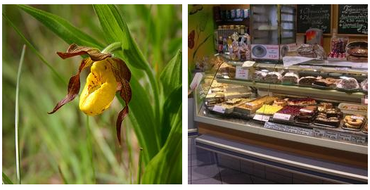
During the training phase, the content dataset chosen for this project comprised 80 images from the COCO (Common Objects in Context) dataset¹⁹. This is one of the largest and most commonly used content datasets for object recognition and instance segmentation. I selected 80 training content images, which mainly include natural scenes and human portraits. All images had a resolution of 512 x 512 pixels. 

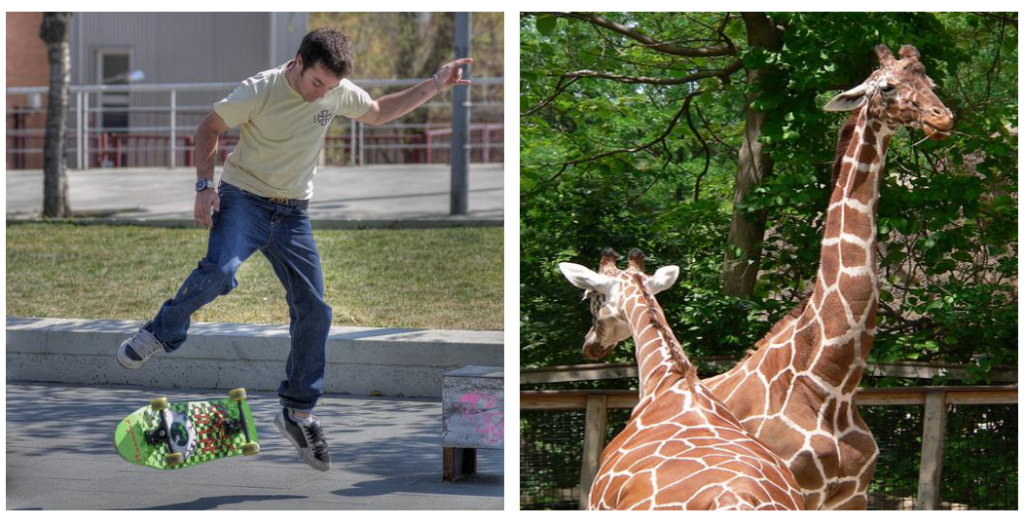
The model’s performance and its ability to generalize to unseen data were evaluated using a separate testing content dataset. This testing content dataset consisted of images used both to calculate validation losses for checkpoint selection and to generate the stylized outputs in the final evaluation, but not for gradient-based parameter updates during training. For the testing dataset, I selected 80 content images from the ImageNet dataset²⁰. 

Style dataset

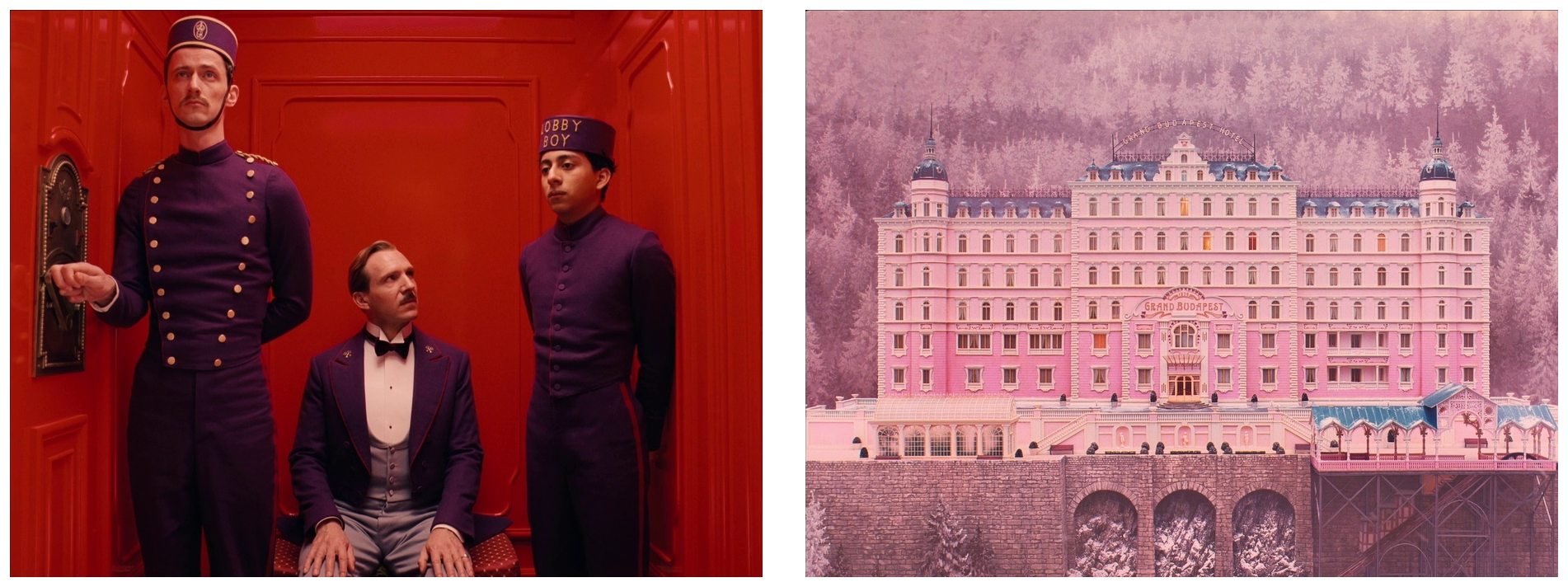
The film-based style dataset utilized in this project was a collection of frames from the movies of two Hollywood directors: Wes Anderson and Tim Burton. These frames were obtained from FilmGrab²¹, a free, carefully curated repository dedicated to movie stills for filmmakers, designers, and students. All the movie frames that were downloaded from FilmGrab²¹ exhibited varying aspect ratios and resolutions due to different cinematic shooting formats. 

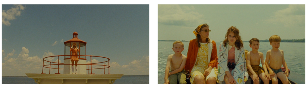
For Wes Anderson, I collected 28 frames sampled from two of his movies: The Grand Budapest Hotel (2014) and Moonrise Kingdom (2012), with exactly 14 frames for each movie. These movie frames were selected with variability to capture Wes Anderson’s signature visual aesthetics. For example, 14 frames selected in The Grand Budapest Hotel include wide shots of the hotel exterior (4 frames) and interior (4 frames), alongside symmetrical character shots (6 frames). 

A similar selection approach was used for 14 frames in Moonrise Kingdom, with 6 symmetrical shots of characters, 6 wide exterior shots, and 2 interior shots. 

For Tim Burton, 28 movie frames were also collected across two of his movies: Beetlejuice (1988) and Alice in Wonderland (2010). Once again, I used the similar selection pipeline to choose 14 frames for each of those two movies. 

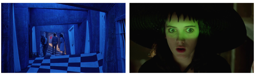
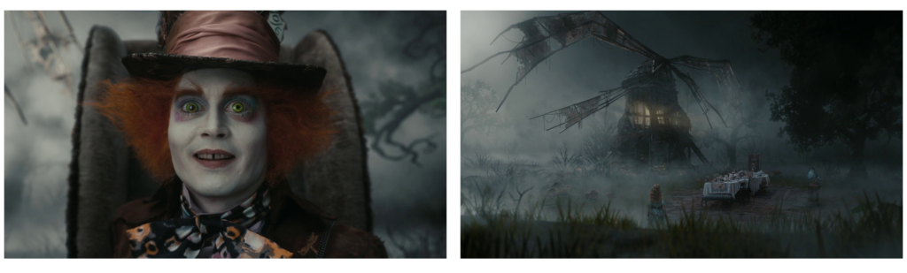
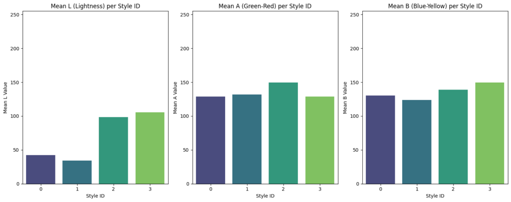
In this study, each set of 14 frames sampled from a single film was associated with a distinct cinematic style, characterized by clearly separate color palettes and lighting conditions. To illustrate this, I computed the mean values of the L, A, and B channels across each movie’s frame set. These three channels are components of the LAB color space: In OpenCV’s 8-bit LAB representation, L measures lightness from 0 (black) to 255 (white), while A and B represent the green–red and blue–yellow color axes, respectively.

Since the model used in this study was inherently a multi-style network capable of learning multiple styles simultaneously, this film-based style dataset was used in both training the model and generating the final stylized results for evaluation. 

Preprocessing

Since both the content and style images had varying aspect ratios and dimensions, they were preprocessed before being fed into the model for training to ensure consistent input distributions. This involved resizing images to 256 x 256 pixels, followed by random cropping to 240 x 240 pixels. All images were then normalized to have mean = [0.485, 0.456, 0.406] and standard deviation = [0.229, 0.224, 0.225] to match the normalization parameters used for ImageNet when training the original VGG-16 network.

Methodology

Standard Neural Style Transfer framework

The standard Neural Style Transfer framework proposed by Gatys et al.¹ used a convolutional neural network pretrained for object classification. The network was composed of various layers where convolutional filters extracted feature representations from the input images. Each layer produced a feature map, representing the activations of those filters.

Gatys et al. discovered that reconstruction of the image from the feature maps at lower layers of the network tended to produce the original pixel-level details of the image, while reconstruction from the feature maps at higher layers could extract high-level content information from the image. Therefore, Gatys and colleagues proposed choosing a single layer conv _ for content representation and a subset of layers conv _ , conv2_ , conv3_1, conv4_1, and conv5_1 for style representation. This multi-scale representation allowed the model to capture both low-level stylistic features and high-level structures, semantic patterns.

The standard framework required using a loss function. This loss function contained two terms—the content loss and the style loss—with their respective weight parameters,  and :

The relative content and style weights determine the balance between content preservation and stylization. The content loss was defined as the squared Euclidean distance between the high-level feature responses of the two images at the layers selected for content reconstruction. Let  and  be the original image and the stylized image, and  and  be their respective feature representation at layer . Then the content loss at layer l was as follows:

With  as the single style-representative image, the style loss at layer l is defined as the mean squared Euclidean distance between the Gram matrices of the two images’ features across layer l:

The total style loss is then summed across all layers selected for style reconstruction, with representing the weighting factors that determine each layer’s contribution to the total style loss:

The Original Multi-Style Transfer Framework of Dumoulin et al.⁴

The multi-style transfer framework built by Dumoulin and colleagues consisted of two components: a feed-forward image transformation network and a frozen loss network. The image transformation network was trained using stochastic gradient descent to minimize the losses computed by the frozen loss network.

The image transformation network was a deep residual convolutional neural network that mapped input images directly to output images. This network largely followed Johnson et al.’s residual architecture but replaced zero-padding with mirror-padding, transposed convolutions with nearest-neighbor upsampling followed by a convolution, and Batch Normalization with Conditional Instance Normalization (CIN).

In this multi-style transfer framework, Conditional Instance Normalization (CIN) was the key factor that enabled multiple styles to be trained simultaneously within a single one feed-forward network. This approach could be achieved using the following equation, which features  as a layer’s activation,  as the style index, and  as the mean and standard deviation taken across spatial axes of , and and as style-specific affine parameters representing style :

and were augmented as matrices, where  is the number of styles and  is the number of output feature maps. For each style being modelled, CIN selected the rows corresponding to the specified style index to retrieve the pair of parameters unique for each style. Then, at each convolutional layer, those style-specific parameters scaled and shifted the content feature map , producing the conditioned activation  that was passed to the subsequent layers of the transformation network. The final layer then converted the learned feature representation into the stylized output.

A frozen loss network was also utilized to encode content and style representations for loss calculations. In the original paper, Dumoulin et al.² used a VGG-16 network⁴ pretrained for object classification. During training, the frozen loss network extracted content representations from the stylized image—which was the output of the image transformation network—and the input content image, and style representations from the stylized image and the reference style image.

Layer relu3_3was selected for content representation, and the subset of layers relu1_2, relu2_2, relu3_3, and relu4_3 was chosen for style representation. These content and style representations were then used to compute the respective content and style losses. Finally, the optimizer was employed to minimize these losses and update the transformation network’s learnable parameters, including the style-specific parameters learned by the CIN.

Applying Cinematic Stylization Using CIN and Gram-Matrix-Based Style Representations

In this study, I implemented two separate experiments, both of which employed the same network architecture as in the original work by Dumoulin et al.⁴ to condition the content feature maps on each pair of style-specific parameters. The network architecture was outlined in the original paper of Dumoulin et al.⁴

Experiment 1: Using a single representative style image for each style being modelled

In the original work by Dumoulin and colleagues, each artistic style was represented by a single image in the style dataset. Similarly, in this experiment, a pre-defined style image was randomly selected for each of the four styles to compute the style losses.

Experiment 2: Computing average Gram matrices from multiple frames

In addition to the first experiment, I also trained a separate model with a modified style loss function. In particular, I explored the average Gram matrices computed from each style’s collection of movie frames as the style representation, then used it as the target in the style loss function.

Given the specified layers for style reconstruction, the loss network extracted feature maps from every style image corresponding to style . Then, for each selected layer, the Gram matrices of the 14 reference frames were summed and averaged across all style images to obtain a single style representation. In particular, let be the  image of style , the average Gram matrices of style  at layer  can be calculated using the following equation:    

            

Then, the average Gram matrix computed at layer l for style representation served as the target for the style loss function at layer .  With as the stylized image rendered in style s and  as its Gram matrix at layer , the style loss function at layer l is as follows:

Training

In both experiments, I explored several content-to-style loss weight ratios and achieved the best content-style balance with a content weight of 1 and a style weight of 10. The model was trained over 300 epochs. In addition to the content loss and the style loss, the total variation loss was also introduced to reduce pixel-level noise in the stylized images. Following Dumoulin and colleagues², a pretrained VGG-16 classifier was used as the loss network. During training, the model was optimized using the Adam optimizer. Once optimization was complete, the network could stylize images in a single forward pass. The network was trained using the hyperparameters outlined in the Appendix’s Table 2.

Both experiments were conducted in Google Colab runtime and implemented using PyTorch 2.11.0. Certain implementation details were inspired by a publicly available GitHub repository²². To account for variability due to stochastic training, each complete experiment was repeated using the same set of random seeds: 11, 22, and 33. The following passages describe the detailed behavior for each experiment per random seed.

Training details of Experiment 1

At the beginning of each seed-specific training run, the frozen VGG-16 network, image-transformation network, and the Adam optimizer were initialized. Next, at each training epoch, a style index was randomly selected from the four available styles and assigned to the entire content batch using one-hot encoding. This style code and the batch were then passed through the image transformation network to obtain their corresponding stylized outputs. Intermediate feature maps were then extracted from the content batch, the pre-defined style image for the selected style, and the stylized batch to compute the content loss, style loss, total variation loss, and the total loss for the batch.

After every 10 epochs, the model was then subsequently evaluated on the testing dataset without parameter updates. During validation, every content image in the testing dataset underwent the same preprocessing procedures as the training content images, but center crops were used instead of random crops to ensure consistent evaluation across runs. Then, these testing images were evaluated under all four styles, and the mean batch-level validation content loss, style loss, total variation loss, and total loss were recorded.

The best model checkpoint was overwritten and saved for each seed whenever the current validation loss improved by at least 0.5% of the previous best validation loss. If no such improvements occurred for five consecutive validation checks, training was stopped to prevent overfitting and save computational resources.  At the end of each epoch-level loop, a record of the current epoch was created, storing information on training losses, training time, and their corresponding validation results. Then, output stylized results for evaluation were generated using the best model checkpoint saved for each seed.

Training details of Experiment 2

The behavior at each random seed for Experiment 2 followed procedures similar to those used in Experiment 1, with the only exception being the calculation of style loss: instead of using the pre-defined style image, it used the average Gram matrices precomputed from each style’s collection of reference frames. Other details were the same as Experiment 1.

Evaluation Methodology

In this study, lighting and color distribution associated with cinematic styles were defined as the statistical distribution of L, A, and B channels across each style’s collection of reference cinematic frames. Specifically, for each testing content image, reference style frame, and their corresponding stylized result, their one-dimensional L-channel, A-channel, and B-channel histograms were calculated, using a 32-bin histogram. Each histogram was then normalized, which converted raw pixel counts into relative frequencies that summed up to 1. This helped ensure that histogram comparisons reflected differences in lighting and color distribution.

Before conversion to LAB color space, both the testing content images and the reference style frames were resized so that their shorter side measured 256 pixels while preserving the original aspect ratio. They were then center-cropped to 240  240 pixels. The stylized results already had a resolution of 240  240 pixels, so no additional resizing or cropping was applied to them during evaluation. These outputs were then denormalized and saved as RGB images before extraction of the L, A, and B channels.

To conduct statistical analysis for lighting and color distribution, the Wasserstein distance was utilized to measure the distance between normalized 1D histograms. This is a metric that measures the minimum cost of transforming one probability distribution into another.

Baseline-relative improvement

To answer RQ1, I modeled the baseline-relative improvement. In particular, for each stylized result and channel, I computed the Wasserstein distance from its normalized one-dimensional channel histogram to each of the 14 reference frames in the same style. These values were then aggregated to produce one channel-specific distance for each generated image. This can be expressed using the following formula, with  as the stylized image and  as the reference frame  belonging to style :

Results were summarized by style, experiment, and seed using the mean and standard deviation. These values were then compared against their content baseline. Since the same testing content images were used to generate stylized results across the three seeds and two experiments, the mean channel-specific distance from each testing content image to each collection of reference style frames was summarized by style across the 80 images without seed or experiment-level aggregation.

Next, the baseline-relative improvement was calculated by subtracting the stylized output’s mean channel-specific distance from the corresponding content image’s distance, using the following formula, with  as the input content image,  as the stylized image, and  as the style index:

Positive values indicated that stylizations moved the inputs closer to the reference-frame distribution, while negative values suggested that they moved the image farther away. For each style, experiment, seed, and channel, the baseline-relative improvement was first averaged across the 80 testing content images and was then summarized across the three seeds using their mean, sample standard deviation, and 95% Student’s t-confidence interval.

Between-experiment difference

To address RQ2, the channel-specific mean Wasserstein distances were compared between the two experiments. For each style, channel, experiment, and seed, the distances obtained from the 80 stylized outputs were summarized to produce one seed-level mean. Then, the three seed-level means were averaged to obtain an overall mean distance for each style-channel-experiment combination.

The experiment with the lower overall mean distance was considered to have produced outputs whose channel-specific distributions were closer to the corresponding reference-frame collection. Therefore, a lower mean distance for Experiment 1 would indicate greater similarity for the single-frame representation, while a lower mean distance for Experiment 2 would indicate greater similarity for the average Gram-matrix representation. These comparisons were conducted separately for the L, A, and B channels.

Results

Training and validation losses recorded for Experiment 1 and Experiment 2

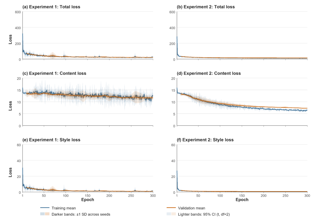
Figure 8 shows training and validation loss curves across three independent seeds 11, 22 and 33 for Experiment 1 and Experiment 2. The content and style loss curves reported the unweighted loss components calculated before applying their respective coefficients, while the total loss reported the weighted sum of the content, style, and total variation loss. Although total variation loss was included in the calculation of the total loss, it was not presented as a separate curve, because it functioned only as a term for reducing pixel-level noise and was not directly related to the research’s objectives.

Across both experiments, training and validation losses generally decreased over 300 epochs. Experiment 2 achieved lower and smoother total, content, and style losses than Experiment 1, with narrower variability across seeds. A clearer downward trend was also observed in Experiment 2’s losses, whereas greater fluctuations were reported for those of Experiment 1. This difference was reported only as a descriptive characteristic of their optimization behavior and was not interpreted as evidence that Experiment 2 improved style-transfer quality. The broadly similar trends in the training and validation losses do not provide clear visual evidence of severe overfitting during training.

Baseline-relative improvement across the L, A, and B channels of the two experiments

Table 1 and Table 2 summarize the channel-specific baseline-relative improvement for each experiment, using their sample mean and standard deviation. Baseline SDs represent variation among the 80 testing images, whereas output and improvement SDs represent variation among the three seed-level means. The improvement intervals were calculated using Student’s t-distribution (n = 3, df = 2). In the tables, Style 0, Style 1, Style 2, and Style 3 denote cinematic stylizations in Alice in Wonderland, Beetlejuice, The Grand Budapest Hotel, and Moonrise Kingdom, respectively.

Table 1 presents the L-channel, A-channel, and B-channel baseline-relative improvement produced by Experiment 1. On average, all the L-channel improvements were positive values, with the largest mean L-channel improvement observed for Style 0 (+14.789 ± 2.881) and the lowest mean improvement for Style 2 (+4.401 ± 0.206). Meanwhile, Style 1 is the only style for which its 95% confidence interval included zero, suggesting that a consistently positive L-channel improvement was not observed for the style. Regarding the A-channel and B-channel baseline-relative improvement results, stylized images rendered in Style 1 produced opposite results across the two channels: their mean A-channel baseline-relative improvement was negative (−2.814 ± 0.340) but their B-channel counterpart was positive (+3.352 ± 0.511). Similarly, Style 0 exhibited inconsistent results across the two channels. Both Style 0’s B-channel confidence interval and Style 3’s A-channel confidence crossed 0, suggesting that no consistent positive improvement was observed for these styles’ color distribution.

Style	Channel	Testing baseline, mean ± SD	Stylized output, mean ± SD	Improvement, mean ± SD	95% CI for mean improvement
Style 0	L-channel	33.502 ± 10.811	18.713 ± 2.881	14.789 ± 2.881	[7.631,21.947]
	A-channel	7.664 ± 4.999	5.795 ± 0.047	1.870 ± 0.047	[1.752, 1.987]
	B-channel	13.056 ± 9.319	14.675 ± 1.232	−1.619 ± 1.232	[−4.680, 1.442]
Style 1	L-channel	36.290 ± 10.910	31.393 ± 2.391	4.898 ± 2.391	[−1.042, 10.837]
	A-channel	11.353 ± 4.903	14.167 ± 0.340	−2.814 ± 0.340	[−3.659, −1.969]
	B-channel	18.818 ± 8.319	15.466 ± 0.511	3.352 ± 0.511	[2.082, 4.621]
Style 2	L-channel	17.266 ± 6.225	12.865 ± 0.206	4.401 ± 0.206	[3.888, 4.913]
	A-channel	22.917 ± 6.895	6.120 ± 0.249	16.797 ± 0.249	[16.179, 17.415]
	B-channel	14.924 ± 6.750	10.381 ± 0.203	4.543 ± 0.203	[4.039, 5.046]
Style 3	L-channel	20.165 ± 5.805	15.476 ± 0.714	4.688 ± 0.714	[2.915, 6.462]
	A-channel	7.898 ± 4.998	6.536 ± 0.809	1.362 ± 0.809	[−0.648, 3.372]
	B-channel	20.299 ± 7.490	6.489 ± 0.059	13.809 ± 0.059	[13.664, 13.955]

Similar to Experiment 1, Experiment 2 produced positive mean L-channel improvements for all four styles, although Style 1’s confidence interval included zero. Positive A- and B- channel improvements were also observed across styles, with all 95% confidence intervals excluding zero. The strongest A-channel improvement occurred for Style 2 (17.045 ± 0.052), while the strongest B-channel improvement occurred for Style 3 (13.363 ± 0.359). Conversely, Style 1 showed the weakest A- and B-channel improvements among all four styles (2.208 ± 0.300 for A-channel and 4.455 ± 0.347 for B-channel).

Style	Channel	Testing baseline, mean ± SD	Stylized output, mean ± SD	Improvement, mean ± SD	95% CI for mean improvement
Style 0	L-channel	33.502 ± 10.811	20.268 ± 3.033	13.234 ± 3.033	[5.698, 20.769]
	A-channel	7.664 ± 4.999	4.472 ± 0.008	3.193 ± 0.008	[3.171, 3.214]
	B-channel	13.056 ± 9.319	5.213 ± 0.065	7.843 ± 0.065	[7.682, 8.003]
Style 1	L-channel	36.290 ± 10.910	29.022 ± 3.290	7.268 ± 3.290	[−0.906, 15.442]
	A-channel	11.353 ± 4.903	9.144 ± 0.300	2.208 ± 0.300	[1.464, 2.953]
	B-channel	18.818 ± 8.319	14.363 ± 0.347	4.455 ± 0.347	[3.592, 5.318]
Style 2	L-channel	17.266 ± 6.225	11.167 ± 0.212	6.099 ± 0.212	[5.573, 6.625]
	A-channel	22.917 ± 6.895	5.872 ± 0.052	17.045 ± 0.052	[16.915, 17.174]
	B-channel	14.924 ± 6.750	8.577 ± 0.063	6.347 ± 0.063	[6.190, 6.504]
Style 3	L-channel	20.165 ± 5.805	14.632 ± 1.563	5.533 ± 1.563	[1.649, 9.416]
	A-channel	7.898 ± 4.998	4.580 ± 0.035	3.317 ± 0.035	[3.230, 3.404]
	B-channel	20.299 ± 7.490	6.936 ± 0.359	13.363 ± 0.359	[12.472, 14.254]

Between-experiment difference

In general, Experiment 2 produced lower mean L-channel distances than Experiment 1 for Style 1, Style 2, and Style 3 and lower mean A-channel distances for all four styles. It also produced lower B-channel distances for all styles except Style 3 (6.489 ± 0.059 for Experiment 1 and 6.936 ± 0.359 for Experiment 2)

Style	Channel	Experiment 1, mean ± SD	Experiment 2, mean ± SD	Lower-distance experiment
Style 0	L-channel	18.713 ± 2.881	20.268 ± 3.033	Experiment 1
	A-channel	5.795 ± 0.047	4.472 ± 0.008	Experiment 2
	B-channel	14.675 ± 1.232	5.213 ± 0.065	Experiment 2
Style 1	L-channel	31.393 ± 2.391	29.022 ± 3.290	Experiment 2
	A-channel	14.167 ± 0.340	9.144 ± 0.300	Experiment 2
	B-channel	15.466 ± 0.511	14.363 ± 0.347	Experiment 2
Style 2	L-channel	12.865 ± 0.206	11.167 ± 0.212	Experiment 2
	A-channel	6.120 ± 0.249	5.872 ± 0.052	Experiment 2
	B-channel	10.381 ± 0.203	8.577 ± 0.063	Experiment 2
Style 3	L-channel	15.476 ± 0.714	14.632 ± 1.563	Experiment 2
	A-channel	6.536 ± 0.809	4.580 ± 0.035	Experiment 2
	B-channel	6.489 ± 0.059	6.936 ± 0.359	Experiment 1

Discussion

The findings indicated that both single-frame and average Gram-matrix style representations produced positive mean L-channel baseline relative improvements across all four styles. This suggested that the stylized outputs of the CIN-based multi-style transfer framework were generally closer to their corresponding reference frames’ lighting distribution than their original images did. Among the four styles, cinematic stylizations from Beetlejuice had the least consistent L-channel baseline-relative improvements across three independent runs as their improvements’ confidence intervals included zero in both experiments.

The results for color distribution were more varied: Experiment 1 produced negative mean improvement in the A-channel for Beetlejuice and in the B-channel for Alice in Wonderland. Moreover, both the improvement intervals for the B channel of Alice in Wonderland and the A-channel of Moonrise Kingdom included zero. In contrast, Experiment 2 produced positive mean improvements in both chromatic channels for all results, with all A- and B-channel improvement intervals excluded zero. Taken together, these results suggested that in both experiments, the CIN-based style transfer model could reproduce measurable lighting and color characteristics, but its effectiveness depended on the style, channel, seed, and original content images.

A comparison of the results from the two experiments revealed that Experiment 2 produced lower distances for most of the evaluated style-channel combinations. In particular, Experiment 2 produced lower A-channel distances for all four styles and lower L- and B-channel distances for three of the four styles. Alice in Wonderland was the exception in the L-channel, while Moonrise Kingdom was the exception in the B-channel. These results indicated that the average Gram-matrix representation generally reproduced the lighting and color distributions of the reference collections more effectively than single-frame style representation. This advantage was most consistent in the A-channel, suggesting that aggregation may have been particularly useful for transferring green-red chromatic distribution. However, as exceptions were still observed in L- and B-channel distances, the effect of Gram-matrix averaging may depend on both the cinematic style and the evaluated channel.

Overall, the CIN-based multi-style transfer framework of Dumoulin and colleagues⁴ produced measurable cinematic lighting and color-transfer changes to images. My findings also supported the average Gram-matrix representation as a promising approach to capture lighting and color distribution associated with cinematic frames, with its produced outputs generally closer to the reference-frame collections.

Several limitations should be considered when interpreting these findings. First, only three random seeds were used to represent independent training runs. This small number contributed to wide confidence intervals under some conditions and limited the certainty of the across-seed estimates. In addition, the dataset was relatively small, and the same testing content images were used for checkpoint selection and final evaluation. Consequently, the reported results may contain selection bias and should not be interpreted as performance on a fully independent test set.

The findings may also depend on the selected CIN-based architecture because the loss network and image-transformation network were adopted from Dumoulin et al.⁴ without substantial modifications. Furthermore, the study evaluated only lighting and color distributions extracted from static frames; it therefore cannot represent cinematic style comprehensively or support conclusions about temporal characteristics such as motion, transitions, and editing patterns. The evaluation was limited to descriptive statistics derived from normalized one-dimensional LAB histograms. These histograms do not capture the joint relationship between the A and B channels, while alternative color spaces such as RGB and HSV could provide complementary information about transferred color characteristics.

I’m also unable to generalize my findings to a broader range of cinematic styles involving other films, directors, or reference-frame selection pipelines. The film-based style dataset only included selected works by Wes Anderson and Tim Burton, with each style represented by 14 frames. The pre-defined reference frames were also randomly selected for single-frame style representation, which may lead to different outcomes with other options of single style representative frames. Therefore, this study could not evaluate whether variation in the choice of director, film, number of reference frames, or frame selection procedure might have influenced the results.

Future research could investigate additional Gram-matrix aggregation strategies and other modifications to the standard style-loss function for styles represented by multiple images. Broader comparisons could include fixed single-frame targets, random-frame sampling, per-film averages, and per-director averages evaluated against held-out frames. Future studies could also examine additional CNN-based architectures, Generative Adversarial Networks²³, and diffusion models²⁴, as well as representations of composition and temporal cinematic characteristics.

Overall, this research contributes to a broader understanding of how convolutional neural networks can represent artistic styles associated with cinema. Results suggested that while aggregated Gram-based style representation more closely reproduced the original cinematic lighting and color characteristics of the reference frames than single-frame, their style-transfer effects were heavily dependent on the style, original content images, and seeds. By exploring neural style transfer through using a film-based style dataset, this study provided an exploratory connection between computational image generation and the analysis of cinematic aesthetics.

Legal Considerations

The cinematic frames were obtained from FilmGrab²¹, a publicly accessible archive that presents film stills under fair use for educational and reference purposes. Copyright remains with the respective rightsholders, and the frames were used solely for non-commercial academic research. This study claims no ownership of the images and credits FilmGrab²¹ and the corresponding films as data sources.

Acknowledgements

I would like to express my gratitude to my research mentor, Dr. Mariel Werner from UC Berkeley, for her support and guidance throughout this research project.

Disclosure of AI-assisted technologies

ChatGPT 5.6 Sol and Codex were consulted solely for general guidance on structuring the statistical analysis. The author independently made all methodological decisions, reviewed and adapted the code, verified the calculations against the source data, interpreted the results, and takes full responsibility for the analysis and conclusions.

Appendix

Symbol	Definition
	Original content image
	Stylized output image
	Cinematic-style index,
	Reference-frame index within a style
	The single style-representative image
	The -th reference frame belonging to style
	Evaluated LAB channel,

Symbol	Definition
	Index of a selected neural network layer
	Activation of the content image at layer
	Activation of the stylized image at layer
	Activation of the reference frame at layer
	Gram matrix calculated from the feature representation of stylized output at layer
	Gram matrix calculated from the feature representation of reference frame at layer
	Average Gram matrix representing style at layer

Symbol	Definition
	Content loss
	Style loss summed across the selected layers
	Style loss calculated at layer
	Weight assigned to the contribution of layer to the total style loss
	Weighted total training loss
MSE	Mean Squared Error
	Weight assigned to the content loss
	Weight assigned to the style loss

Symbol	Definition
	Input activation map to a CIN layer
	Mean of the activation map across its spatial dimensions
	Standard deviation of the activation map across its spatial dimensions
	Style-specific scaling parameter used by CIN
	Style-specific shifting parameter used by CIN
	Output activation produced by CIN
	Number of styles represented by the CIN parameter matrices
	Number of output feature maps in a CIN layer

Symbol	Definition
	Normalized histogram of channel extracted from stylized image
	Normalized histogram of channel extracted from original content image
	Normalized histogram of channel extracted from reference frame
	Mean channel-specific distance between stylized image and the reference frames of style
	Mean channel-specific distance between content image and the reference frames of style
	Channel-specific baseline-relative improvement
	Wasserstein distance between two normalized histograms
	Number of independent seed-level values used across-seed summaries;
	Degrees of freedom for the Student’s t-interval

Setting	Value
Input size	240 240 3
Number of cinematic styles	4
Padding mode	Reflection padding
Normalization	Conditional Instance Normalization after every convolution
Optimizer	Adam
Learning rate	10-3
Adam parameters	β1 = 0.9, β2= 0.999
Maximum training duration	300 epochs
Approximate maximum parameter updates	3000
Batch size	8
Content-loss weight	1
Style-loss weight	10
Total-variation-loss weight	10-5
Validation interval	Every 10 epochs
Random seeds	11, 22, and 33
Convolution initialization	PyTorch default Conv2d initialization (Kaiming uniform)
CIN offset initialization	βs​∼N(0,0.01)
CIN scale initialization	γs ∼ N(μ = 0, σ = 0.01)
Loss network	Frozen ImageNet-pretrained VGG-16
Content-reconstruction layer	relu3_3
Style-reconstruction layers	relu1_2, relu2_2, relu3_3, and relu4_3

References

1. L. A. Gatys, A. S. Ecker, M. Bethge. Image style transfer using convolutional neural network. 2016 IEEE Conference on Computer Vision and Pattern Recognition (CVPR), pg. 2414–2423, 2016, https://doi.org/10.1109/CVPR.2016.265 [↩] [↩]
2. K. Simonyan & A. Zisserman. Very deep convolutional networks for large-scale image recognition. arXiv preprint arXiv:1409.1556. https://doi.org/10.48550/arXiv.1409.1556 [↩]
3. J. Johnson, A. Alahi, L. Fei-Fei. Perceptual losses for real-time style transfer and super-resolution. Computer Vision – ECCV 2016. Vol. 9906, pg. 694–711, 2016, https://doi.org/10.1007/978-3-319-46475-6_43 [↩] [↩]
4. V. Dumoulin, J. Shlens, M. Kudlur. A learned representation for artistic style. International Conference on Learning Representations (ICLR), 2016, https://doi.org/10.48550/arXiv.1610.07629 [↩] [↩] [↩] [↩] [↩] [↩] [↩] [↩]
5. D. Chen, L. Yuan, J. Liao, N. Yu, G. Hua. Stylebank: an explicit representation for neural image style transfer. 2017 IEEE conference on computer vision and pattern recognition (CVPR), pg. 2770–2779, 2017, https://doi.org/10.1109/CVPR.2017.296 [↩] [↩]
6. Y. Li, C. Fang, J. Yang, Z. Wang, X. Lu, M. H. Yang. Diversified texture synthesis with feed-forward networks. 2017 IEEE conference on computer vision and pattern recognition (CVPR), pg. 266–274, 2017, https://doi.org/10.1109/CVPR.2017.36 [↩] [↩]
7. H. Zhang & K. Dana. Multi-style generative network for real-time transfer. European Conference on Computer Vision, pg. 349–365, 2018, https://doi.org/10.1007/978-3-030-11018-5_32 [↩] [↩]
8. H. Ikuta, K. Ogaki, Y. Odagiri. Blending texture features from multiple reference images for style transfer. SA’16: SIGGRAPH ASIA 2016 Technical Briefs, pg. 1–4, 2016, https://doi.org/10.1145/3005358.3005388 [↩] [↩] [↩]
9. A. Sanakoyeu, D. Kotovenko, S. Lang, B. Omme. A style-aware content loss for real-time style transfer. Proceedings of the European Conference on Computer Vision (ECCV), pg. 698–714, 2018, https://doi.org/10.48550/arXiv.1807.10201 [↩] [↩] [↩]
10. I. Zabaleta & M. Bertalmío. Photorealistic style transfer for cinema shoots. 2018 Colour and Visual Computing Symposium (CVCS), pg. 1–6, 2018, https://doi.org/10.1109/CVCS.2018.8496499 [↩] [↩]
11. F. Luan, S. Paris, E. Shechtman, K. Bala. Deep photo style transfer. Proceedings of the IEEE Conference on Computer Vision and Pattern Recognition (CVPR), pg. 4990–4998, 2017, https://doi.org/10.1109/CVPR.2017.740 [↩]
12. D. Parmar. Framing and composition in films of Wes Anderson, 2020 [↩] [↩]
13. S. Lee. Wes Anderson’s ambivalent film style: the relation between mise-en-scène and emotion. New Review of Film and Television Studies, 14(4), pg. 409–439, 2016, https://doi.org/10.1080/17400309.2016.1172858 [↩]
14. S. İnceoğlu & Ö. Gündem. Architect or director? Wes Anderson with his cinematic spaces. Gazi University Journal of Science Part B: Art Humanities Design and Planning, 12(4), pg. 619–634, 2024 [↩]
15. Attademo. Color and/is narration. The narrative role of color in Wes Anderson’s filmic images. Cultura e Scienza del Colore-Color Culture and Science, 13(01), pg. 7–13, 2021 [↩] [↩]
16. R.S. Humaida. The impact of the characteristic of Tim Burton’s music and cinema on one’s personality. Humanities & Language: International Journal of Linguistics, Humanities, and Education, 1(1), pg. 35–41, 2023, https://doi.org/10.32734/kafayd86 [↩]
17. S. Schäfer, C. Weidner, B.E.M Style. The dark side of a genius: the influence of German expressionism on Tim Burton. Film in Context, pg. 1–17, 2012. Retrieved from https://www.academia.edu/10477231/The_Dark_Side_of_a_Genius_The_Influence_of_German_Expressionism_on_Tim_Burton_2012_ [↩]
18. Z. Qin. A study of film aesthetics of Tim Burton–Taking Alice in Wonderland as an example. Proceedings of the 2nd International Conference on Interdisciplinary Humanities and Communication Studies. Vol. 21, pg. 163–168, 2023, https://doi.org/10.54254/2753-7064/21/20231456 [↩]
19. T.Y. Lin, M. Maire, S. Belongie, L. Bourdev, R. Girshik, J. Hays, P. Perona, D. Ramanan, C. L. Zitnick, P. Dollár.  Microsoft coco: common objects in context. European conference on computer vision, pg. 740–755, 2014. https://doi.org/10.48550/arXiv.1405.0312 [↩]
20. J. Deng, W. Dong, R. Socher, L.J. Li, K. Li, L. Fei-Fei. Imagenet: a large-scale hierarchical image database. 2009 IEEE conference on computer vision and pattern recognition, pg. 248–255, 2009, https://doi.org/10.1109/CVPR.2009.5206848 [↩] [↩]
21. https://film-grab.com/ [↩] [↩] [↩] [↩]
22. I. Goodfellow, J. Pouget-Abadie, M. Mirza, B. Xu, D. Warde-Farley, S. Ozair, A. Courville, Y. Bengio. Generative adversarial networks. Advances in Neural Information Processing Systems (NIPS), pg. 2672–2680, 2014, https://doi.org/10.48550/arXiv.1406.2661 [↩]
23. I. Goodfellow, J. Pouget-Abadie, M. Mirza, B. Xu, D. Warde-Farley, S. Ozair, A. Courville, Y. Bengio. Generative adversarial networks. Advances in Neural Information Processing Systems (NIPS), pg. 2672–2680, 2014, https://doi.org/10.48550/arXiv.1406.2661 [↩]
24. J. Sohl-Dickstein, E. Weiss, N. Maheswaranathan, S. Ganguli. Deep unsupervised learning using nonequilibrium thermodynamics. International conference on machine learning, pg. 2256–2265, 2015, https://doi.org/10.48550/arXiv.1503.03585 [↩]