Numerical Exploration of HOBO vs. QUBO: Using Sudoku as a Benchmark

Abstract

Sudoku, with its complex combinatorial structure, provides a natural NP-hard benchmark for testing optimization models. In this study, we quantitatively compare Quadratic Unconstrained Binary Optimization (QUBO) and Higher-Order Binary Optimization (HOBO). While QUBO is compatible with quantum computers, it is often evaluated on classical simulators known as quantum simulators which calculates with tensor network executed on GPU instead of actual quantum, due to current hardware noise. Conversely, HOBO — an emerging formulation currently restricted to quantum simulators — extends interactions beyond quadratic terms, theoretically offering more compact models and expanded search space. To evaluate these advantages, we systematically tested puzzle sizes (4×4, 8×8, and 9×9) with blank-cell ratios from 10% to 50%. This upper limit was selected because resolvability drops to 0% for 9×9 cases beyond 50%, while smaller grids lose solution uniqueness, invalidating comparison. The results reveal that HOBO consistently outperforms QUBO in smaller grids (4×4, 8×8) where variable efficiency is pronounced. However, in 9×9 cases, the auxiliary range penalty required for HOBO reduces its advantage and performing worse than QUBO in some cases. This illustrates that HOBO’s benefits are context-dependent: dominant in compact settings but limited when range penalty is required. By clarifying these trade-offs, our work provides a framework for maximizing HOBO’s efficiency, with broad analysis implicating its potential when utilized in the quantum computer. Ultimately, this research underscores the necessity of tailoring the mathematical formulation to the specific structural constraints of the problem to maximize the performance of next-generation optimization solvers.

Keywords: Sudoku, Higher-Order Binary Optimization, QUBO, tensor-network sampler, NP-hard problems

Introduction

First, quantum computing is defined as a mathematical formulation programming that can be executed in either real quantum computers or quantum simulators^1,2,3,4. Quantum computing falls into two categories: quantum annealing and quantum gate. While quantum annealing approaches have gained traction^5,6, different methods are required to execute the mathematical formulations in quantum computers or quantum simulators.

Quantum computing has made remarkable progress in addressing combinatorial optimization problems, with QUBO (Quadratic Unconstrained Binary Optimization) among the most widely studied formulations^7,8. QUBO is the most orthodox algorithm which has modeled diverse tasks such as the Traveling Salesman Problem and Shift Scheduling^{9,10,11,12,13}. Nonetheless, its strict reliance on quadratic binary interactions introduces structural bottlenecks. These limitations motivate broader frameworks that encode richer constraint systems more compactly. In this context, Higher-Order Binary Optimization (HOBO) allows interactions beyond quadratic terms^7,9,10,11,8. We investigate these principles on Sudoku.

The objective of this study is to quantitatively examine when HOBO’s theoretical advantages—bit reduction and expansion of search space gains—manifest and under what conditions they may diminish. Therefore, this is not an experiment to address whether HOBO provides advantages compared to the Sudoku solvers, since Sudoku is just one example of NP problem which is perfect for this experiment. In particular, we probe regimes that include larger grids for which some constraints are naturally implemented as quadratic range penalty, a modeling choice that can interact with higher-order encodings. Rather than optimizing for absolute speed or solver-specific performance, we seek a formulation-level understanding of how encoding choices shape the search space.

To that end, we design a systematic evaluation across three grid sizes (4 × 4, 8 × 8, 9 × 9) and five blank-cell ratios (10%, 20%, 30%, 40%, 50%). This factorial setup allows us to study scaling and constraint regimes separately from instance idiosyncrasies. We employ a tensor-network–based sampler to explore energy landscapes under both formulations, track variable counts and explore the relationship between sparsity and success rate, and maintain comparable penalty weighting policies across conditions to isolate encoding effects.

Related Work

Limitations of Standard QUBO Encodings

While Quantum Annealing has successfully addressed various combinatorial tasks^14,15,16, Hamada et al.¹⁷, the standard QUBO framework presents significant scalability challenges for complex logic puzzles. The conventional approach, formalized by Glover et al.¹⁸, relies on mapping constraints to quadratic penalties. For problems with non-binary domains^19,10, such as Sudoku (where a cell holds values 1–9), this necessitates “one-hot” encoding. Lucas¹ demonstrated that while this method is universally applicable, it is resource-intensive. Representing a variable with D possible states requires D qubits. Furthermore, enforcing exclusivity constraints (selecting exactly one state) demands all-to-all connectivity within those qubits, resulting in O(n³) physical couplings for problem size n. Tamura et al.²⁰ noted that this inflation creates rugged energy landscapes plagued by local minima, making it difficult for annealers to locate feasible solutions without extensive use of auxiliary (ancilla) qubits.

HOBO and Tensor Networks

To mitigate the qubit overhead of one-hot encodings, recent research has pivoted toward HOBO. This framework permits k-body interactions (k > 2), allowing for compact binary encodings that scale logarithmically (n × n × log₂ n) rather than linearly with domain size²¹. Chancellor et al.⁷ proposed architectures where these multi-body terms could theoretically be implemented, smoothing the energy landscape by reducing the volume of invalid states.

However, current physical hardware is largely restricted to pairwise (quadratic) interactions. Consequently, the evaluation of HOBO formulations has shifted toward classical simulation using Tensor Networks. Orús¹² and Markov & Shi¹³ established that tensor contractions could efficiently simulate quantum states with limited entanglement, providing a viable testbed for verifying HOBO performance before large-scale high-order hardware becomes available.

Sudoku as a Constraint Density Benchmark

Sudoku serves as a rigorous benchmark for these encoding schemes due to its strict “hard constraints,” where a single violation renders a solution invalid. Previous quantum approaches have predominantly utilized the QUBO’s one-hot method²² or hybrid quantum backtracking²³. While these studies confirm solvability, they rarely address the efficiency trade-offs between encoding types as problem size scales.

Methods

Sudoku Rules and Examples

Sudoku is a popular logic-based, combinatorial number-placement puzzle. The objective is to fill a grid with digits so that each column, each row, and each of the designated blocks contain all of the digits without repetition. Sudoku puzzles come in various sizes, with the most common being the 9 × 9 grid divided into 3 × 3 blocks.

Although there are several types of Sudoku puzzles, the standard rules are:

• Each Row: Must contain each digit exactly once.
• Each Column: Must contain each digit exactly once.
• Each Block: Each designated block must contain each digit exactly once.

Sudoku follows logical rules to ensure a unique solution; however, in challenging puzzles, it may be necessary to make a hypothesis by assuming the value of a cell to solve the entire puzzle.

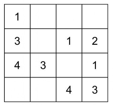
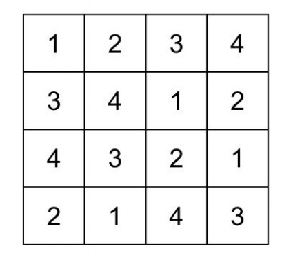
To illustrate the concept, consider a smaller 4 × 4 Sudoku puzzle. The grid is divided into four 2 × 2 blocks. The digits to be placed are 1 through 4. In this puzzle, the goal is to fill the empty cells so that each row, column, and 2 × 2 block contains all of the digits from 1 to 4 exactly once.

The smaller grid size makes it easier to manually solve and understand the application of the Sudoku rules. By applying logical deductions based on the given numbers and constraints, one can fill in the missing digits to complete the puzzle. For example, this puzzle can be solved, initially starting from the third row, eventually filling all of the cells.

Problem Setup for 9×9 Sudoku

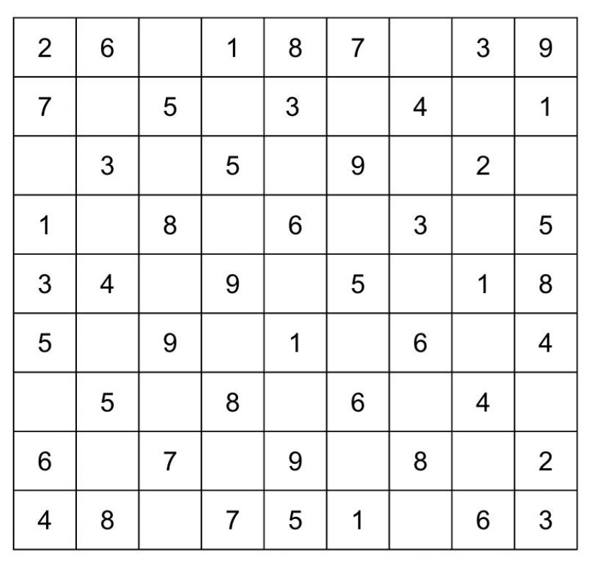
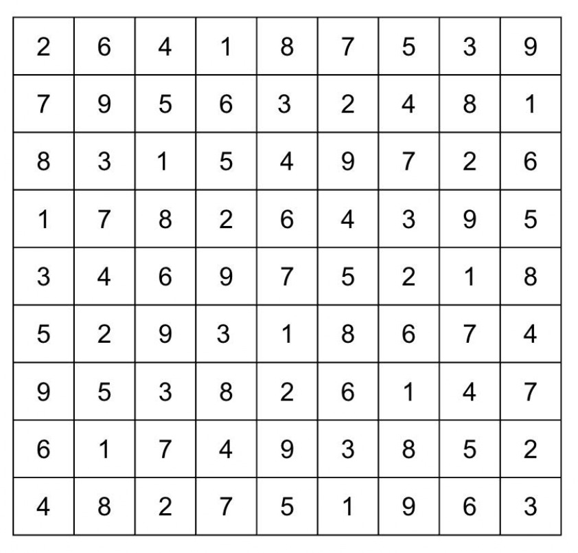
The objective is to populate the blanks with numbers from 1 to 9, ensuring each row, column, and block contains unique values. We encoded blank cells as 0 and substituted specific values for the provided numbers, applying the constraints outlined below. We tested our HOBO formulation on a standard 9 × 9 Sudoku puzzle:

As illustrated above, logical reasoning and systematic understanding enable us to fill in the puzzle starting from the bottom line, ultimately completing the entire grid. To solve this using HOBO, we translated the five mathematical constraints into Python code. We represented the using for loops and encoded the numbers 1–9 with 4-bit representations, while enforcing a cell constraint to exclude numbers 10–16.

Study Scope, Instance Generation, and Difficulty Levels

Target Sizes and Blank-Cell Rates

We consider three Sudoku sizes: 4 × 4, 8 × 8, and 9 × 9. 8 × 8 Sudoku puzzle is similar to 4 × 4 and 9 × 9, but the only difference is that the block constraint is rectangle instead of square. For every size, puzzles are generated by the same procedure, and blank cells are placed at five difficulty levels: 10%, 20%, 30%, 40%, and 50%. As mentioned before, our experiment ends by 50% due to the limitations within both HOBO and QUBO in 9×9, which they can not provide an optimal solution after 50%, and multiple possible solutions for smaller sizes, which forces the controlled group to be uncontrolled. This design enables comparisons under consistent conditions across both grid size and difficulty.

Common Instance-Generation Procedure

We sourced valid, solved Sudoku grids from the Kaggle Sudoku dataset to ensure logical consistency for the difficulty level of empty cells. We then applied our own masking algorithms (Sparse and Clustered) to these solved grids to generate the specific blank-cell ratios required for testing.

Mathematical Formulation and Objective

The Sudoku puzzle can be formulated as a constraint satisfaction problem, where each cell must contain a unique number, and each number must appear exactly once per row, column, and block²⁴. We introduce five constraints and minimize their violations for 9 × 9 Sudoku puzzle:

   

Cell Constraint

   

for i in range(size):
for a, b in combinations(range(size), 2):
Hconst += (1 - (q[i][a][1] - q[i][b][1])**2) * (1 - (q[i][a][0] - q[i][b][0])**2)

Here, bits are binary; (i, j) indexes a cell and 0, 1, 2, 3 are exponents of 2. This penalizes numbers from 10 to 16 so the values remain within 9 for 9 × 9 Sudoku.

Row Constraint

   

for i in range(size):
for a, b in combinations(range(size), 2):
Hconst += (1 - (q[i][a][1] - q[i][b][1])**2) * (1 - (q[i][a][0] - q[i][b][0])**2)

This enforces uniqueness across each row by penalizing identical values at different column positions.

Column Constraint

   

for j in range(size):
for i1, i2 in combinations(range(size), 2):
Hconst += (1 - (q[i1][j][1] - q[i2][j][1])**2) * (1 - (q[i1][j][0] - q[i2][j][0])**2)

This enforces uniqueness across each column by penalizing identical values at different row positions.

Block Constraint

   

# size = 9x3
for br in range(0, size, 3):
for bc in range(0, size, 3):
block_nodes = [q[r][c] for r in range(br, br+3) for c in range(bc, bc+3)] for a, b in combinations(block_nodes, 2):
Hconst += (1 - (a[1] - b[1])**2) * (1 - (a[0] - b[0])**2)

This prohibits identical values within the same 3 × 3 block via higher-order interactions. This formulation is slightly different from QUBO formulation, because HOBO can be formulated with binary numbers therefore, to formulate “not a same number”, the binary characteristics is utilized in this formulation. This penalizes when two cells carry identical 4-bit patterns. By multiplying each digit, if there is a same number, the penalty is 1, which does the exact same function as XOR. This contributes significantly to the reduced terms of the formulation compared to QUBO. However, since QUBO represents each number without the usage of binary, so it requires ancilla bits to represent until 9.

Substitution Constraint

   

The indicator applies the constraint only where givens exist; mismatches with fixed bits are penalized.

HOBO’s Additional Formulation for Output

Higher-Order Binary Optimization (HOBO) is designed to tackle binary optimization problems involving inter-actions beyond quadratic terms. While QUBO focuses solely on quadratic interactions between binary variables19, HOBO expands this scope to include third-order and higher interactions, enabling more expressive constraints.

Binary Representation of Numbers

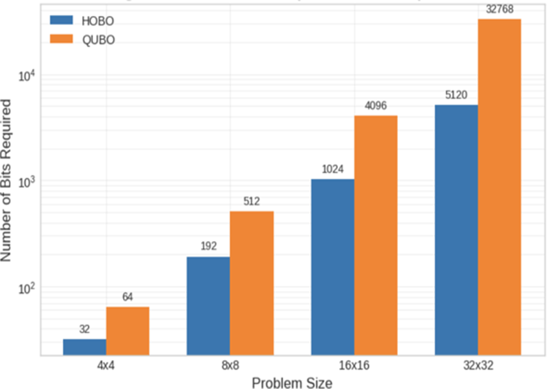
Utilizing HOBO’s characteristics, we represented the value of numbers in binary form (4 bits for 1–9), reducing the quantum bits by half relative to one-hot. This limits the number of variables to n × n × log₂n, whereas QUBO requires n × n × n. The representation decreases variables and can improve runtime and accuracy.

Uniqueness in Binary (Row-wise Example)

To prohibit duplication without auxiliary one-hot variables, we directly penalize equality across all bits:

   

This penalizes when two cells carry identical 4-bit patterns. The same idea extends to columns and blocks.

Hconst += (1 - (q[0][0] - q[1][0])**2) * (1 - (q[0][1] - q[1][1])**2)
Hconst += (1 - (q[0][0] - q[2][0])**2) * (1 - (q[0][1] - q[2][1])**2)
Hconst += (1 - (q[0][0] - q[3][0])**2) * (1 - (q[0][1] - q[3][1])**2)
Hconst += (1 - (q[1][0] - q[2][0])**2) * (1 - (q[1][1] - q[2][1])**2)
Hconst += (1 - (q[1][0] - q[3][0])**2) * (1 - (q[1][1] - q[3][1])**2)
Hconst += (1 - (q[2][0] - q[3][0])**2) * (1 - (q[2][1] - q[3][1])**2)

This code represents the uniqueness in binary in both row and column. It is important to note that although the math equation starts the count from 1, the code starts the count from 0. By utilizing this basic formulation, it is possible to represent row, column and block constraint.

Limiting the Range of Values

Binary coding may represent undesired numbers (e.g., 6–8 with 3 bits). We penalize specific bit-patterns to restrict the range, e.g., to 1–5:

   

Hconst += 10 * (q[i][j][0] * q[i][j][1] + q[i][j][0] * q[i][j][2])

This does not directly solve Sudoku but is a reusable building block as puzzle size changes. This formulation is the so-called range penalty which limits values from 10-16 (9-15 in code). This formulation suppresses invalid values (10–15) by exploiting their binary structure. In a 4-bit encoding, values 8 through 15 all have the most significant bit (q₃, representing 2³=8) set to 1. Specifically, values 10 (1010₂) and 11 (1011₂) share bits q₃ and q₁. Values 12 (1100₂) through 15 (1111₂) share bits q₃ and q₂. By penalizing the products q₃q₁and q₃q₂, we selectively inhibit the range 10–15 without affecting valid digits 1–9.

QUBO Formulation and Conversion

QUBO can also express Sudoku in mathematical formulations. It can be even easier than HOBO, due to its characteristics of one-hot encoding.

   

This represents that the number of each cell is restricted from 1 to 9.

   

The equation penalizes same numbers across the same row.

   

Likewise, this equation penalizes same numbers across the same column.

   

   

This equation restricts same numbers across the same block, contributing as a block constraint. As mentioned before, this differs from HOBO’s block constraint because QUBO can not represent a number as binary. The difference in formulas is mathematically necessary and ensures the comparison is fair. The formulas differ because the two methods utilize fundamentally different variable encodings: QUBO uses one-hot encoding (requiring summation constraints), while HOBO uses binary encoding (requiring product/difference constraints). Using the same formula for both is impossible because the HOBO formula violates the mathematical definition of QUBO (it is non-quadratic), and using the QUBO formula for HOBO would negate the bit-reduction advantage that the study aims to test.

Comparative Analysis of Computational Resources and Penalty Configurations

This study compares the proposed Higher-Order Binary Optimization (HOBO) and Quadratic Unconstrained Bi-nary Optimization (QUBO) formulations in terms of computational resource requirements and penalty configurations. The analysis specifically focuses on the effective resource consumption for the target Sudoku instance, where fixed cells are treated as constants, leaving only 8 blank cells as variables.

Table I presents the penalty coefficients (Lagrange multipliers, λ) configured for each formulation. Although penalty coefficient for cell constraint differs, this does not affect the fair comparison because coefficients are used to balance the weight of the equation, hence, has no impact on the ability of samplers.

Constraint Type	HOBO (λ)	QUBO (λ)
Cell Constraint	10	1
Row Constraint	1	1
Column Constraint	1	1
Block Constraint	1	1
Substitution (Fixed Cells)	N/A	N/A

In the HOBO formulation, the Cell Constraint coefficient is set significantly higher (λ = 10). This is due to the nature of binary encoding; four qubits can represent values from 0 to 15, but Sudoku requires values in the range 0 to

8. The penalty for values 9 through 15 must be strictly enforced to ensure valid integers before evaluating the puzzle rules. Conversely, in the QUBO formulation, the “one-hot” constraint functions with equal weight to other structural constraints (λ = 1), as it is inherently integrated into the quadratic energy landscape.

Table 1 details the actual resource requirements for the specific problem instance with 8 blank cells. The actual bits differ from the theoretical bits due to substitution constraint, because some cells already possess a number while others may be blank.

In the HOBO formulation, the Cell Constraint coefficient is set significantly higher (λ = 10). This is due to the nature of binary encoding; four qubits can represent values from 0 to 15, but Sudoku requires values in the range 0 to

8. The penalty for values 9 through 15 must be strictly enforced to ensure valid integers before evaluating the puzzle rules. Conversely, in the QUBO formulation, the “one-hot” constraint functions with equal weight to other structural constraints (λ = 1), as it is inherently integrated into the quadratic energy landscape.

Table 2 details the actual resource requirements for the specific problem instance with 8 blank cells. The actual bits differ from the theoretical bits due to substitution constraint, because some cells already possess a number while others may be blank.

Metric	HOBO	QUBO
Bits per Cell	4	9
Blank Cells	8	8
Actual Bit Count	32	72
Logic Constraints	980	251

Interaction Degree High (∼ 8) Quadratic (2)

As demonstrated in Table 2, the HOBO formulation achieves a significant reduction in the logical qubit count (32 qubits) compared to QUBO (72 qubits). This reduction is critical for current quantum hardware and simulators, as it drastically shrinks the solution search space. However, a trade-off exists regarding the number of logical constraints. The HOBO formulation requires 980 constraints because it utilizes a pair-wise comparison method (9 choose 2 = 36 pairs per row, column, or block) to ensure unique values.

In contrast, the QUBO formulation utilizes a summation-based approach (sum of x_ijk – 1), resulting in only 251 constraints. Although HOBO introduces higher-order interactions that may increase compilation overhead, the substantial reduction in the number of required qubits makes it a highly effective approach for instances with a limited number of empty cells.

Implementation with TYTAN Solver

We employ a tensor-network-based sampler to explore energy landscapes^12,13,25. The TYTAN solver acts as a classical simulator for quantum annealing operating through iterative bit-flipping mechanics. The solver’s execution is controlled primarily by two parameters: shots and T_num. The shots parameter represents the number of independent trials, yielding the total sample size. Therefore, we have decided to use success rate as the dependent variable, which represents the number of shots that have reached to optimum solution. Conversely, T_num defines the number of iterations (or steps) performed per single shot, effectively determining the resolution of the Simulated Annealing-based flip schedule.

While flip schedules can vary among different solvers, TYTAN applies a unified schedule for both QUBO and HOBO formulations. Within the duration defined by T_num, the flipping dynamics evolve: bit flips are actively executed during the initial 50% of the iterations, whereas the process shifts to perform two flips per step during the final stages of the annealing cycle. For performance evaluation, both formulations are compiled via samplers, and the average wall-clock time is measured over five random seeds in a GPU environment.

Software and Environment

The optimization models were implemented using Python 3.9 and the TYTAN SDK (version 0.0.18), specifically utilizing the hobotan module for symbolic Hamiltonian construction. Random seeding and matrix manipulations were handled using NumPy. In our HOBO formulation, the Hamiltonian is constructed such that the ground state energy corresponds to zero constraint violations. The TYTAN solver outputs a negative Ising energy and if it is the negative value of offset, it is optimal solution.

   

No numerical tolerance was applied; any state with was classified as a failure.

Results

Experimental setup and logging format

We evaluated the same Sudoku instance with both formulations under a matched sampling budget. For each formulation, we fixed shots to 10,000, T_num to 100,000 and repeated the experiment across five random seeds {0, 1, 2, 3, 4}, resulting in an aggregate of 10,000 × 100,000 × 5 internal flip proposals. Here, T_num denotes the number of iterations attempted; it is the 0/1 flip schedule defined by the TYTAN solver’s author and was used as provided. The flips occur for the first 50% of the total iterations and it will be 2 flips per step near the end. All runs were executed on GPU, and energies are reported exactly as returned by the sampler together with the occurrence counts. To document what a successful run looks like, we include representative sampler outputs for each formulation; these are illustrative excerpts showing the reported offset, the top energy level(s), and a reconstructed board for visual inspection. Aggregated behavior by blank rate and board size is summarized in Figure. 6–8 and described in paragraphs dedicated below. To note, the number of blank cells was adjusted by the rounded number to engage in a fair environment for different sizes.

Output for HOBO

The excerpt below shows a typical HOBO run where the sampler reports the compile-time offset and then lists the top energy encountered with its occurrence count, followed by a reconstructed candidate board. The energy −192.0 matches the offset magnitude and is the minimum value observed for this instance; the displayed board satisfies the Sudoku constraints for rows, columns, and blocks. The value of offset will be different from QUBO, because the mathematical formulations are different, hence, the difference in the number of terms and powers lead to the distinct offset. Occurrence counts indicate how many times that exact minimum was sampled within 10,000 shots. Thus, for this example, only 11 optimal shots were executed, however, this is a significant result because quantum computing emphasizes the ability to execute optimal solution and not the success rate. This format is repeated for each seed under the same fixed budget; we show two excerpts here to illustrate the logging style and the shape of a correct solution.

Offset 192.0

   

   

Output for QUBO

The next excerpt shows a typical QUBO run under the same computational budget. The sampler reports an offset of

128.0 and lists the best energy −128.0 with its occurrence count alongside another near-optimal energy levels. Each printed array is a reconstructed candidate board corresponding to the stated energy; the minimum-energy board satisfies all Sudoku constraints for this instance. As with HOBO, multiple seeds were evaluated and produce similar logs; we include one representative block to illustrate the offset, energy lines, and the format of the reconstructed boards. These excerpts serve as concrete records of what the sampler returns under our fixed shots and T_num choices.

Offset 128.0

   

   

Success Rate Analysis: 9×9 Grid

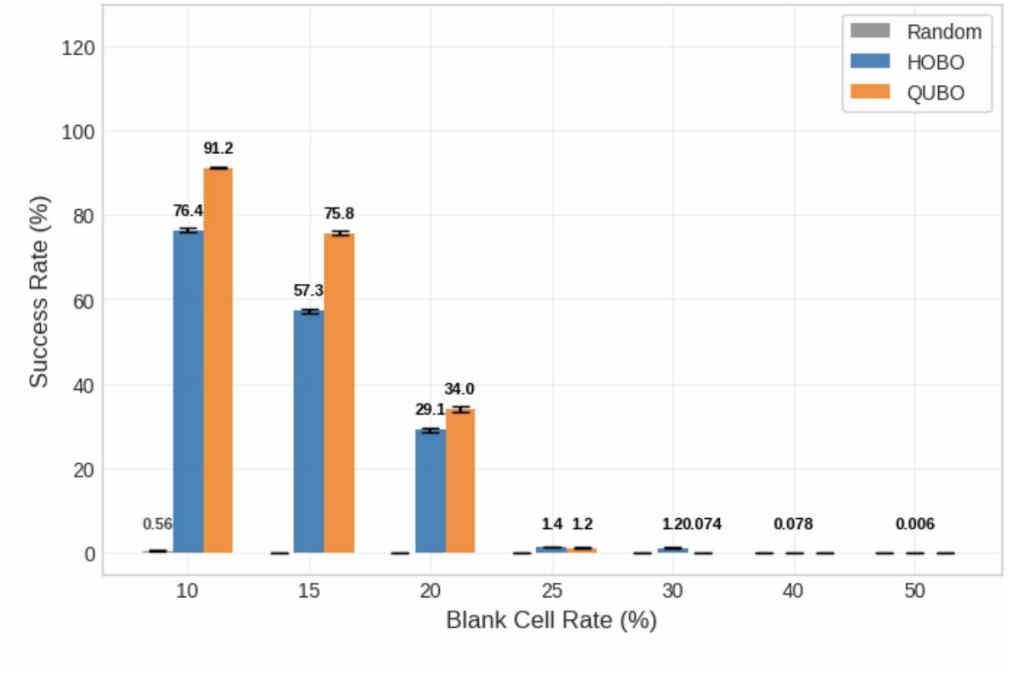
Figure 6 summarizes the ratio of optimal solutions sampled as the blank-cell rate increased on the 9×9 board. At 10% and 15% blanks, the recorded success rates are higher for QUBO; by 20%, both counts have decreased, but QUBO still reports a larger value in the plotted dataset. Starting at 25% blanks, the HOBO bar exceeds the QUBO bar and the difference widens as sparsity grows in the figure. At 40% blanks, QUBO shows zero success rate in the plotted run, while HOBO retains a small but nonzero success rate; at 50% blanks the chart annotates a single HOBO hit with a success rate of 0.002%. This represents the limitation and further improvements required for HOBO solvers. However, this is important in quantum computing, because the fact whether optimal solution is executed matters and not the rate. For example, random guessing is displayed as 0% successful, which implies the significance for HOBO for reaching to an optimal solution. Ultimately, Statistical testing confirms QUBO’s significant lead at 10-20% blank rates (p < 0.001). However, the crossover at 25% marks a significant shift, with HOBO outperforming QUBO from 25% through 40% (p < 0.001). At 50%, while HOBO retains unique solutions, the difference is not statistically significant (p = 0.08) due to the extreme scarcity of successful samples.

Success Rate Analysis: 4×4 Grid

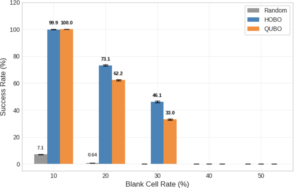
Figure 7 reports success rates (optimal hits divided by shots) for the 4×4 board across blank-cell rates. In the 10–30% range, both methods achieve near-ceiling rates, and the plotted bars are closely matched. At 40% blanks, the success rate declines relative to the easier cases, with HOBO’s bar remaining higher in the figure; at 50% blanks, the same pattern persists with both rates reduced compared to the 10–30% region. The chart uses a common vertical axis across methods to make the absolute levels comparable and to highlight where separation appears. Furthermore, T-tests reveal no statistically significant difference between the methods in the 10-30% range (p > 0.05), indicating parity on easier instances. However, as difficulty increases to 40% and 50% blanks, HOBO significantly outperforms QUBO (p < 0.001), supporting the hypothesis that compact encoding aids search under sparsity. Overall, this figure establishes the small-board baseline under which both encodings are capable of frequent exact recoveries.

Success Rate Analysis: 8×8 Grid

Figure 8 presents success rates for the 8×8 board at blank-cell rates of 10%, 20%, and 30%. At 10% blanks, both formulations reach essentially perfect success in the plotted dataset. At 20% and 30% blanks, the HOBO bars are higher than the QUBO bars, showing a consistent margin at these mid-range difficulties. For completeness, trials at 40% and 50% blanks were conducted but both methods recorded zero success in the underlying data and those points are omitted from the figure for readability. This mid-scale chart connects the near-ceiling behavior of 4×4 with the count-based view of 9×9 by displaying the percentage outcomes under an intermediate size. Lastly, statistical analysis confirms that while QUBO holds a slight edge at 10% (p < 0.001), HOBO demonstrates a statistically significant advantage at 20% and 30% blank rates (p < 0.001 in both cases), validating the visual margin observed in the mid-range difficulty.

Blank Rate (%)	Backtracking (s)	QUBO (s)	HOBO (s)
10%	∼ 0.01	4.10	3.00
20%	∼ 0.01	4.50	3.70
30%	∼ 0.01	7.80	7.20
40%	∼ 0.01	11.30	13.50
50%	∼ 0.01	17.80	21.30

Computational Time

Table 3 shows the average execution times for each size. For reference, a standard backtracking solver solves the same 4×4 instance within 0.01 seconds. While the annealing approach involves significant overhead due to formulation complexity, the number of shots and T_num is the major reason, therefore, if the shots are significantly decreased, it can be reduced to around 1 second. For 8×8 and 9×9, standard backtracking solves these instances in <0.05s. We omit the full comparison table for larger sizes because the classical backtracking advantage is already established in the 4×4 case, and the focus of this study is the relative difference between HOBO and QUBO, not beating classical silicon. The table also shows the faster computational time for QUBO over HOBO as the blank cells increase, which is due to the difference in the solvers. HOBO requires complex solvers which are adapted for higher order terms, significantly different from QUBO. To reiterate, the importance is the execution of optimal solutions, therefore, the main purpose should be focused on the success rate, while this does provide a further field of improvement for HOBO.

Discussion

About Energy Graph

The intuition behind the curves in Figure 8 is simple. HOBO maintains a higher proportion of valid digit encodings overall, so far more of its raw bit patterns already correspond to concrete digits; a sampler does not constantly “fall off” the space of valid numbers. QUBO’s one-hot flips, in contrast, frequently create 0-hot or 2-hot states, so many steps are spent repairing cells before row/column/block consistency can even be addressed. As blanks increase, progress depends less on single-cell fixes and more on coordinating digits across lines and blocks; because HOBO’s base-2 flips always produce a digit, a higher share of its steps carry useful information forward.

The energy surface also differs: HOBO’s cooperative high-order penalties create broad, smoother slopes toward feasibility, which helps the “last mile” from a nearly correct board to an exact solution, whereas QUBO’s pairwise penalties produce many small ridges and pockets that encourage jitter and plateaus. One caveat is unique to 9×9: HOBO must include range penalties to forbid overflow codes (9–15), and those cell-level barriers can slow early repairs when givens are plentiful; this explains why QUBO can look better at 10–20% blanks before HOBO’s structural advantages and smoother geometry reassert a clear advantage as sparsity grows.

Implications from the Graphs

Figure 6 (9×9 counts). The success rate plot shows the characteristic split: QUBO leads in the easy regime (10–20% blanks) with higher success rates, while HOBO overtakes and sustains the tail beyond 20%. At 25–30% blanks, HOBO’s success rate is already larger, and by 40–50% the gap becomes qualitative: HOBO still lands optimal solutions (33 hits at 40%, a single hit at 50%), whereas QUBO drops to zero. This tail behavior is a signature of the smoother HOBO landscape: once the board is almost correct, cooperative penalties guide the last moves into place. However, our results in the 9 × 9 case indicate that simply increasing problem size does not linearly scale this advantage. The introduction of range penalty to limit 4-bit variables (0–15) to the digits 1–9 reduces the fraction of valid cell states, creating energy barriers that hinder search efficiency. Especially, although beating QUBO, we have to acknowledge that HOBO has an incredibly low success rate in blank cells from 25% to 40% ranging from 1.4% success rate to 0.006%success rate. This is primarily due to the combination of the increment of blank cells and range penalty. Nevertheless, the fact that optimal solutions are executed is the most important fact from the graph, because the algorithm’s efficiency is judged based on the ability to produce an optimal solution or not, especially, for quantum computing. Therefore, while the high rate of blank cells and range penalty had crucial influence on the low success rate, the execution of optimal solution outweighs the success rate.

This suggests HOBO is most effective when domain sizes align closely with powers of two. The early QUBO lead aligns with the 9×9-specific burden of range penalties for HOBO, which introduce heavy boundaries that slow simple repairs even though HOBO remains structurally more permissive overall. Read together, the early and late regimes reconcile representation, geometry, and the cell-level range effect without contradiction.

Figure 7 (4×4 success). Both methods sit near the ceiling at 10–30% blanks, confirming that the instance is easy enough for either encoding to succeed rapidly. As the puzzle thins to 40–50%, HOBO’s curve declines gently while QUBO falls faster, leaving a clear margin at the same shot budget. The difference here isolates the cell-level story cleanly: no range penalties are needed, so HOBO’s richer valid-state coverage and smoother energy translate directly into higher success. The result says that more of HOBO’s proposals remain meaningful even when information is scarce, which reduces the time spent on “housekeeping” and accelerates the last-mile convergence. Practically, 4×4 functions as a control that makes the mechanism visible without confounders.

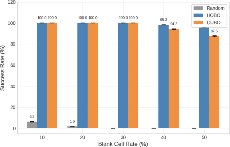
Figure 8 (8×8 success). At 10% blanks both methods are again essentially perfect, but by 20–30% HOBO keeps a consistent margin that matches the “more meaningful steps” narrative. This scale is large enough that coordination across rows and columns matters, yet not so under-specified that all structure dissolves; in this band HOBO’s structural advantages and smoother energy yield a measurable, repeatable benefit. Beyond 40% both encodings fall to 0%, which we attribute to under-specification rather than an encoding failure—there simply is not enough information for either surface to guide the sampler within 50k shots. The fact that HOBO’s lead appears before the collapse indicates that the benefit accrues while information is still actionable. In short, 8×8 connects the clean 4×4 story to the structured 9×9 curve in a way that highlights the same causes at a mid scale.

Effect of Blank-Cell Distribution

Parameters				QUBO (Opt %)		HOBO (Opt %)
Shots	Tnum	Blank Rate	# of Blank	Sparse	Clustered	Sparse	Clustered
50000	100000	30%	5	99.996	81.454	99.988	84.778
50000	100000	30%	19	33.046	12.460	46.076	35.424
50000	100000	30%	24	0.740	0.000	1.196	0.010

Table 4 summarizes the experimental results comparing QUBO and HOBO under two different blank-cell place-ment patterns: clustered and sparse, with a fixed blank ratio of 30% across all puzzle sizes (4×4, 8×8, and 9×9).

To systematically control the spatial distribution of blanks, we designed two deterministic placement patterns. The result is calculated as an average of 5 trials.

Clustered pattern.

Blank cells were added starting from the center of the grid and expanded outward in a clockwise spiral. The central cell was removed first, followed by its surrounding neighbors in circular order. Once a full ring was completed, the process continued to the next outer layer. This produced a compact, center-focused cluster of blanks.

Sparse pattern.

Blank cells were added from the outermost layer of the grid. Specifically, we removed cells at the four corners and the midpoints of each edge first, proceeding clockwise. Each “layer” consisted of eight cells. After completing one layer, the next inner layer was processed in the same manner. This created a uniformly dispersed pattern of blanks across the grid.

For the 4×4 case, both QUBO and HOBO achieved near-perfect optimal solution rates in the sparse condition (QUBO: 99.996%, HOBO: 99.988%). When blanks were clustered, performance declined for both methods, with HOBO (84.778%) slightly outperforming QUBO (81.454%). Although the difference is modest at this scale, it already suggests that HOBO is more robust to unfavorable blank placement.

The effect becomes more pronounced for the 8×8 puzzles. With sparsely distributed blanks, HOBO achieved a 46.076% optimal solution rate, compared to QUBO’s 33.046%. Under clustered placement, both methods suffered, but HOBO (35.424%) still significantly outperformed QUBO (12.46%). This indicates that HOBO’s higher-order interactions exploit globally distributed constraints more effectively than QUBO’s pairwise formulation.

The strongest contrast appears in the 9×9 case. With sparse blank placement, HOBO found 598 optimal solutions out of 50,000 shots (1.196%), while QUBO achieved only 37 (0.074%). Under clustered placement, QUBO failed to find any optimal solutions, whereas HOBO still identified 5 solutions (0.01%). Although absolute success rates are low in this hardest regime, the relative advantage of HOBO remains substantial.

These results demonstrate that not only the number of blank cells but also their spatial distribution critically affects optimization performance. Sparse placement activates row, column, and block constraints more uniformly across the grid, allowing HOBO’s higher-order terms to cooperatively propagate information and eliminate infeasible configurations. In contrast, clustered blanks leave large regions under-constrained, limiting the effectiveness of both methods—especially QUBO’s pairwise interactions.

Overall, the experiments provide quantitative evidence that “where the holes are” is nearly as important as “how many there are,” and that HOBO benefits far more from balanced clue distributions than QUBO. Future studies should therefore explicitly incorporate spatial sparsity patterns, such as layer-based or entropy-based dispersion measures, when evaluating higher-order optimization methods on structured combinatorial problems.

Bit Economy

A second driver of the observed gaps is plain bit economy. HOBO’s compact values reduce the number of binary variables and couplers the sampler must manage, so a larger fraction of each shot goes into negotiating real Sudoku structure rather than repairing one-hot mishaps. This is most obvious in Figure 7, where success stays near the ceiling even as blanks rise, but it also underpins the persistent margin at 20–30% in Figure 8. Even in 9×9, where HOBO’s per-cell density is not perfect and range penalties add friction, the lower variable count helps preserve a tail of discoveries (Figure 6). Operationally, bit economy does not just save memory; it widens the portion of the state space that is worth visiting under a finite-shot budget. That is exactly the regime of our comparisons and why HOBO’s advantage appears as higher success at the same number of samples rather than only as an asymptotic claim.

Practical Guidance for New Instances

For new datasets, the figures suggest a simple playbook. If blanks and dispersion look like the 4×4 and 8×8 bands in Figure 7–8, expect HOBO to lead immediately—almost every move remains meaningful and the surface is smooth—so minimal schedule tuning is required. If an instance resembles early 9×9 in Figure 6 (10–20% blanks with many givens), remember that HOBO’s range penalties make boundary updates heavy; begin with gentler range weights and ramp them only after clear row/column/block structure forms. If puzzle design is under your control, prefer evenly dispersed givens over clustered ones; this makes HOBO’s advantage more visible and stabilizes success across random seeds. Finally, read curves the same way we do here: high baselines and gentle decay in Figure 7 indicate that cell-level density dominates; mid-scale splits in Figure 8 reveal how often moves are truly useful; and hard tails in Figure 6 diagnose whether the landscape helps or hinders last-mile convergence. These habits reduce brittleness, improve reproducibility, and make the HOBO-vs-QUBO choice easier to justify.

Adaptation of Sudoku Problem to Societal Problems

None of the mechanism is Sudoku-specific. The same ingredients—greater search space at the variable level, base-2 flips that remain meaningful, a smoother cooperative surface, and fewer bits—carry directly to assignment-style problems such as TSP with subtour suppression, Latin squares, and graph coloring in dense regimes^{23,20,21,24,26,27,22}. In these settings, a large share of one-hot patterns are wasted states, whereas a compact value code turns far more proposals into bona fide candidates; from a sampler’s perspective, the “useful” portion of the space feels wider. As constraints spread across the graph, cooperative penalties help the last-mile convergence, just as in the tails of Figure 6. Where range-like restrictions are unavoidable (the 9×9 situation), gentle scheduling—start light and anneal—can avoid early blocking while still enforcing correctness later. Together, these parallels explain why the qualitative advantages seen in Figure 2–4 should reappear beyond Sudoku under finite-shot budgets.

Conclusion

This study shows that higher-order binary optimization (HOBO) provides a principled and practically effective alternative to quadratic encodings (QUBO) for Sudoku, and more broadly for discrete problems whose feasibility structure is intrinsically multi-way. The core reason is qualitative: at the cell level HOBO yields a far larger feasible-density ratio than one–hot QUBO, which contracts the effective search space and increases the probability that generic samplers spend shots in useful neighborhoods. Empirically, this density advantage translates into performance at small and mid scales: with a fixed shot budget, HOBO sustains near-perfect success on 4×4 and preserves a persistent margin on 8×8 (Figs. 3–4), despite using many fewer variables (e.g., 324 vs. 729 on 9×9). On 9×9, where range penalties are required to suppress overflow codes, the advantage narrows in easy regimes but reasserts itself as instances become information-sparse: HOBO maintains nonzero discovery probabilities at 40–50% blanks while QUBO collapses (Figure 7). A complementary, instance-level determinant is dispersion: when blanks are evenly distributed across rows, columns, and blocks, HOBO’s cooperative high-order terms prune entire infeasible faces at once, amplifying its gains; clustered blanks weaken this effect. Taken together, these results support a practical rule: prefer HOBO when domain sizes are near powers of two, constraint pressure is diffuse, and global all-different structure dominates; accept QUBO when givens are dense and pairwise exclusions already define straight downhill paths. Limitations remain—most notably schedule and scale calibration in 9×9 with range terms—and point to clear next steps: dispersion-stratified evaluation, sample-efficiency curves, and adaptive penalty normalization/decimation to convert HOBO’s density advantage more reliably into realized gains. Beyond Sudoku, the same density-and-geometry logic suggests that HOBO should be especially valuable for assignment/permutation models, Latin squares, dense graph coloring, and tour problems, where admissible configurations occupy a minute fraction of the ambient binary space and curvature concentrated by native high-order penalties can materially improve search.

Acknowledgements

The authors thank Yuichiro Minato for his guidance on quantum computing applications and Shoya Yasuda for his insightful advice regarding the mathematical analysis and experimental design. We also thank Quantum Fabric Inc. for providing the computational resources required for this study. The computational experiments were performed using publicly available solver libraries, and the authors are grateful to the developers of these tools for making them accessible to the research community.

References

1. A. Lucas. Ising formulations of many np problems. Frontiers in Physics, 2:5, 2014. [↩] [↩]
2. T. Kadowaki, H. Nishimori. Quantum annealing in the transverse ising model. Physical Review E, 58(5):5355, 1998. [↩]
3. T. Albash, D. A. Lidar. Adiabatic quantum computation. Reviews of Modern Physics, 90(1):015002, 2018. [↩]
4. E. Crosson, D. A. Lidar. Prospects for quantum enhancement with diabatic quantum annealing. Nature Reviews Physics, 3(7):466–489, 2021. [↩]
5. S. Yarkoni, et al. Quantum annealing for industry applications: introduction and review. Reports on Progress in Physics, 85(10):104001, 2022. [↩]
6. M. W. Johnson, et al. Quantum annealing with manufactured spins. Nature, 473(7346):194–198, 2011. [↩]
7. N. Chancellor, S. Zohren, P. A. Warburton. Circuit design for multi-body interactions in superconducting quantum annealing systems with applications to a scalable architecture. npj Quantum Information, 3(1):21, 2017. [↩] [↩] [↩]
8. W. Lechner, P. Hauke, P. Zoller. A quantum annealing architecture with all-to-all connectivity from local interactions. Science Advances, 1(9):e1500838, 2015. [↩] [↩]
9. A. Mandal, et al. Compressed quadritization of higher order binary optimization problems. Scientific Reports, 10(1):1–14, 2020. [↩] [↩]
10. I. Hen, F. M. Spedalieri. Driver Hamiltonians for constrained optimization problems. Physical Review Applied, 5(3):034007, 2016. [↩] [↩] [↩]
11. T. Byrnes, J. Freedman, Y. Yamamoto. Generalized Grover’s algorithm for multiple target states. Physical Review A, 83(2):022317, 2011. [↩] [↩]
12. R. Orús. A practical introduction to tensor networks: Matrix product states and projected entangled pair states. Annals of Physics, 349:117–158, 2014. [↩] [↩] [↩]
13. I. L. Markov, Y. Shi. Simulating quantum computation by contracting tensor networks. SIAM Journal on Computing, 38(3):963–981, 2008. [↩] [↩] [↩]
14. E. Farhi, et al. A quantum adiabatic evolution algorithm applied to random instances of an NP-complete problem. Science, 292(5516):472–475, 2001. [↩]
15. K. Srinivasan, et al. Efficient quantum algorithm for solving travelling salesman problem: An IBM quantum experience. arXiv preprint arXiv:1805.10928, 2018. [↩]
16. D. Goldsmith, et al. Beyond QUBO and HOBO formulations, solving the travelling salesman problem on a quantum boson sampler. arXiv preprint arXiv:2406.14252, 2024 [↩]
17. N. Hamada et al. Practical effectiveness of quantum annealing for shift scheduling problem. IEEE International Conference on Quantum Computing and Engineering (QCE), 123–130, 2022 [↩]
18. F. Glover, G. Kochenberger, Y. Du. A tutorial on formulating and using QUBO models. 4OR, 17:335–371, 2019. [↩]
19. B. Palma, et al. QUBO formulation for a nurse scheduling problem: An application for sales force scheduling. IEEE International Conference on Quantum Computing and Engineering (QCE), 123–130, 2022 [↩]
20. K. Tamura, et al. Performance comparison of typical binary-integer encodings in an Ising machine. IEEE Transactions on Computers, 70(8):1250–1261, 2021. [↩] [↩]
21. A. Glos, A. Krawiec, Z. Zimborás. Space-efficient binary optimization for variational quantum computing. npj Quantum Information, 8(1):39, 2022. [↩] [↩]
22. S. Mucke. A simple QUBO formulation of Sudoku. arXiv preprint arXiv:2403.04816, 2024. [↩] [↩]
23. R. Seidel, et al. Quantum backtracking in Qrisp applied to Sudoku problems. arXiv preprint arXiv:2402.10060, 2024. [↩] [↩]
24. T. Hao, et al. A quantum-inspired tensor network algorithm for constrained combinatorial optimization problems. Frontiers in Physics, 10:906590, 2022. [↩] [↩]
25. G. Vidal. Efficient classical simulation of slightly entangled quantum computations. Physical Review Letters, 91(14):147902, 2003. [↩]
26. Z. Tabi, et al. Quantum optimization for the graph coloring problem with space-efficient embedding. IEEE Transactions on Quantum Engineering, 1:1–12, 2020. [↩]
27. K. Domino, et al. Quadratic and higher-order unconstrained binary optimization of railway rescheduling for quantum computing. Quantum Information Processing, 21(9):337, 2022. [↩]