Machine Learning Surrogate Modeling for Aerodynamic Optimization of Idealized Camera-Mirror Housing Geometries

Abstract

This study investigates geometrically simplified automotive camera-based side-mirror designs made with surrogate-assisted modeling. The side-mirror design is not intended to fully replicate a realistic version, but to provide a simplified design space measurable for testing and experimenting. SU2 was used to develop a CFD system to generate 1000 simulations, in which streamlined shapes were represented by modified geometric parameters. Pytorch was also implemented to develop a feedforward neural network meant to predict the drag coefficient from the parameters. The model achieved a test coefficient of determination (R²) of 0.843 and a root mean squared error (RMSE) of 0.082. The surrogate model becomes significantly less reliable in areas with fewer samples in the design space. Targeted validation proved to display unreliable predictive accuracy on high-drag areas and extreme cases when compared to its much more trustworthy results from low-drag areas. The results of the study prove that surrogate-based CFD testing can be an efficient option when enacting an explorative automotive study, but numerical sensitive studies call for higher-level CFD testing to allow for automotive design conclusions.

Keywords: Computational fluid dynamics; surrogate modeling; neural networks; aerodynamic optimization; automotive engineering
Introduction

Introduction

At high speeds, aerodynamic drag plays a critical role in automotive efficiency, as energy consumption depends almost entirely on drag forces¹. Interest in reducing aerodynamic impact in side-mirror design has significantly risen as the automotive industry slowly separates from traditional side-mirrors to camera-based mirror systems. However, high-fidelity computational fluid dynamics (CFD) simulations are computationally expensive², causing many researchers to choose more inexpensive options for exploration-based study. Surrogate modeling has been frequently used as an alternative when paired with machine learning, as it enables quick prediction of aerodynamic properties solely based on geometric parameters³. Exterior mirror geometry and mounting configuration has been shown to strongly influence local flow separation, wake development, aerodynamic loading, and aeroacoustic behavior from past aerodynamic research. Zaareer and Mourad discovered the large alterations of aerodynamic forces and noise generation that can stem from minor geometric changes while studying the influence of side-mirrors⁴. This specific work has been largely expanded to include actual geometric optimization of automotive side-mirrors. Rahman et al. combined turbulent CFD with adjoint-based shape optimization of side-view mirror geometries⁵, while Sankarapandian et al. more specifically studied the optimization of outside rear-mirrors dealing with passenger car drag reduction⁶. Changes to mirror geometry have also been shown to alter separated wake structures and aerodynamic behavior associated with them through biometric surface modification studies.⁷. Fu and Li further proved the sensitivity of mirror wakes through their experimental examination of the wake of a generic automotive side-mirror with modification on its support geometry⁸.

The aerodynamic and aeroacoustic properties of side-mirror geometries continue to be studied through further advanced and detailed numerical and experimental methods. Zaareer et al. proved the idea that shifts and changes in base orientation also significantly alter radiated noise and aerodynamic forces using computational aerocaoustic simulations to optimize the mirror base’s orientation.⁹ Chode et al. used a hybrid computational aeroacoustic method to demonstrate both aerodynamic drag and noise generation’s reliance on mirror configuration while investigating a generic squareback vehicle’s inclined side-mirror configurations.¹⁰ Uhl et al. provided one of the most computationally efficient broadband noise-prediction methods by assessing a vehicle side-mirror’s noise-source modeling for computational aeroacoustic analysis.¹¹ Yemenici and Vatansever Ensarioğlu used combined numerical and experimental assessments to further analyze optimized automotive side-mirror geometries.¹² All these previous studies prove the dependence of mirror aerodynamic behavior on geometry arrangement. They further provide the recommendation of including wake behavior and aerodynamic loading when considering mirror-design review.

In broad terms, the high expenses involved with traditional CFD-based optimization have increased the importance of computational and data-based methods when evaluating aerodynamic design. Neural networks, transfer learning, reduced-order models, and multi-fidelity are commonly used by researchers for aerodynamic coefficients and flow field predictions. Ideal aerodynamic surrogate models have been built by multi-fidelity deep and convolutional neural networks^13,14. Another common method used by studies to predict transonic flow fields and other related aerodynamic quantities is the use of deep-learning architectures^15,16,17. Surrogate-assisted aerodynamic shape optimization has been made significantly more feasible with these developments. Optimization, geometric representations, and sampling strategies have become commonly paired with learned aerodynamic models to increase efficiency when searching excessively complex aerodynamic design spaces^18,19,20,21. Data-driven modeling has been even further advanced beyond traditional feedforward surrogate architectures in recent research. Eiximeno et al. predicted changes in a Windsor body’s pressure field with high-fidelity simulation data while using a variational-autoencoder-based surrogate.²² Shukla et al. developed a DeepONet surrogate capable of predicting aerodynamic flow fields and incorporated the model into constrained aerodynamic shape optimization.²³ More recently, Pereira et al. combined convolutional neural-network aerodynamic prediction with generative modeling in an end-to-end framework for rapid aerodynamic shape optimization.²⁴ These studies prove the decreasing expense involved with recurrent physics-based aerodynamic experiments that stem from the broadening scale of machine learning architecture applicability. Ensemble-learning surrogates, learned geometric representations, adaptive machine-learning optimization, and multi-fidelity surrogate-assisted strategies for aerodynamic design have all been thoroughly studied by researchers for their promising role in future aerodynamic studies.^{25,26,27,28,29} Even though the efficiency of surrogate predictions is beneficial, the studies warn against its reliability in regions with lower sample quantity, and suggest optimized candidates to still be confirmed with physics-based simulation. In this study, a general surrogate-assisted design concept was applied to a simplified automotive camera-based side-mirror housing, also using geometric containment constraints and independent CFD verification of the surrogate selected candidate.

This study also implements both neural network surrogate modeling and a CFD-based dataset to test the level of effect teardrop-inspired geometries have on aerodynamic drag. The goal is to find important geometric patterns and understand how reliable surrogate modeling is when it comes to drawing conclusions about automotive design.
Our hypothesis was that balanced geometries would cause a decrease in overall drag, while more bluff or slender geometries would cause less reliable aerodynamic results. We also hypothesized that the neural network surrogate model would correctly predict CFD-computed drag coefficients when working with the sampled design space.

Methods

Geometry Parameterization

A low-dimensional ellipsoidal parameterization intended to estimate streamlined teardrop-inspired aerodynamic forms was used to generate three-dimensional geometries simplified to create a controlled design space. Four design variables were implemented to control the parameterized geometry,

(a,b,c,d),

where a represents the length of the airflow housing, b represents the width of the housing, c represents the starting vertical thickness, and d represents a thickness-scaling parameter. The generated CFD geometry’s vertical thickness that was used when constructing it was defined as

c_eff = cd.

Correspondingly, the CFD meshing procedure used a, b, and c_eff as the three spatial scale factors meant to control the dimensions. The geometry isn’t changed by parameter d‘s dimension, but by its thickness modifications. The surrogate model used c_eff, instead of c and d independently, using the combined derived geometric features. Unless otherwise stated, thickness in the Results and Discussion refers to c_eff. Figure 1 depicts the parameterized housing geometry and the camera-containment constraints used throughout the study.

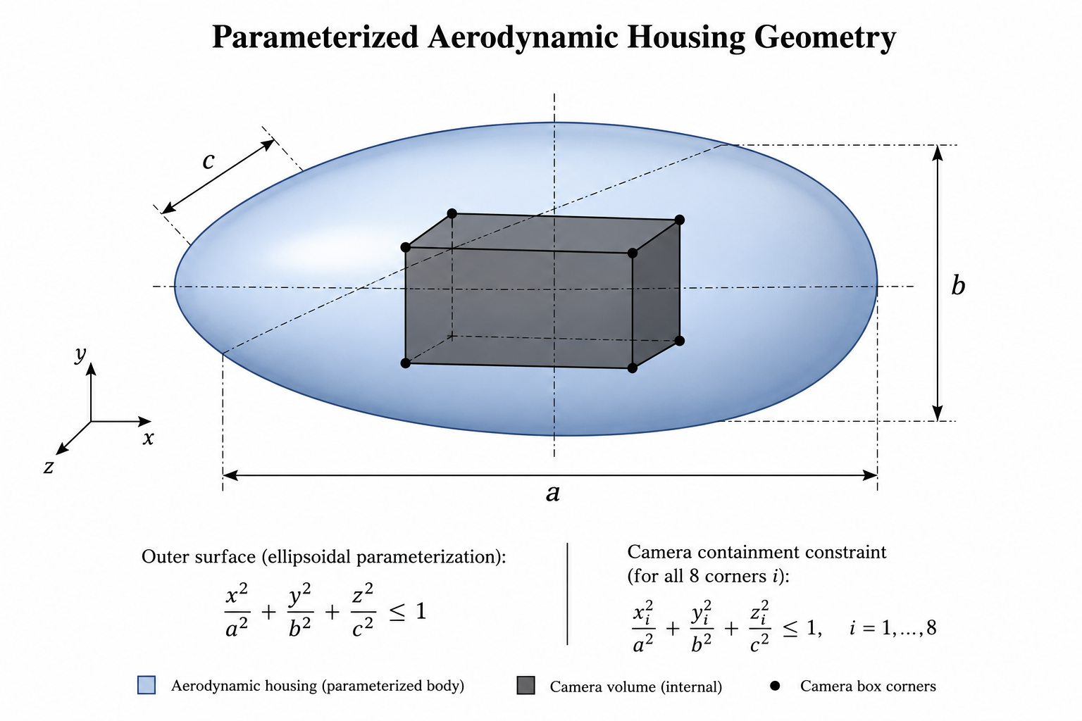
The simplified housing geometry was created as an ellipsoid-like design space that fulfilled

This representation serves as a compact design space with limited dimensions that allows for systematic CFD sampling, surrogate-model training, and constrained gradient-based optimization. This study was not intended to recreate a realistic automotive side-mirror. Instead, to allow efficient observation of aerodynamic trends and optimization behavior, the simplified housing design inspired by camera-based mirror systems used for testing. Despite its simplifications, the housing design is still properly able to capture geometric features that have effects on drag behavior, such as length, thickness, and frontal length. To make sure the simplified geometry produced reliable results, a camera-fit constraint was used. The camera assembly was modeled as a rectangular prism, using dimensions

Instead of implementing solely dimensional limits, all eight corner points of the rectangular prism were evaluated against the housing constraint equation to verify that the camera assembly was fully contained.

For all camera corner points, the value of containment was evaluated as

The geometric constraint function was then used to identify if any corners were outside of the housing barriers:

A parameter set was only considered functional if

This condition determines if all corners lay inside the parameterized housing. If the corresponding parameter set will be declared unusable and rejected because at least one corner lies outside the housing restriction.

As an explicit example of the containment criterion, consider a candidate with , , and . For the centered rectangular camera used here, all eight corner evaluations give a violation of 0.1281, resulting in .

Because , the candidate is considered infeasible and rejected, due to at least one corner of the camera lying outside the ellipsoidal housing.

CFD Simulation Setup

Gmsh was utilized to generate computational meshes and the SU2 solver was used to execute steady-state incompressible flow simulations³⁰. The simulations were conducted under steady freestream conditions, with a constant inlet entering at a velocity of 10 m/s and far-field boundary conditions applied at the domain boundaries. A no-slip condition was used on each of the geometry’s surfaces.
For each geometry, a projected frontal reference area dependent on the geometry was used to ensure the drag coefficient accounts for its size,

where is the lateral width and is the effective thickness.

where is the lateral width and is the effective thickness. The reference length was set to 1.0 m, the freestream velocity was 10 m/s, and the dynamic viscosity was Pas. Drag was taken along the streamwise -direction while aerodynamic forces were tracked on the pod’s surface. This study does not reconstruct dimensional drag force, as a specific numerical density value was not specified from the simulation configuration.

Each simulation used the same numerical setup to generate the original 1000-case dataset and was also run for 200 solver iterations. Later, the additional CFD used to validate surrogate-optimized candidates was run for 1000 iterations. A simplified laminar formulation was modeled to allow batch simulation of a large number of geometries to be enacted efficiently. This approach gives consistent relative comparisons in the parameterized design space, despite not being able to determine all turbulence effects.

Parameter	Value
Solver	SU2 Incompressible Navier-Stokes
Flow velocity	10 m/s
Simulation type	Steady-state
Dataset simulations	200 iterations
Optimized-geometry validation	1000 iterations
Mesh generator	Gmsh
Number of samples	1000

The same CFD procedure was used across all 1000 samples. This procedure included using the same simulation domain, boundary conditions, numerical settings, and meshing methods. Using these same systems reduced variations in the calculated drag values between cases. Each of the 1000 simulations encountered 10 m/s freestream velocity and was run for 200 solver iterations. Since identical conditions were used, the results could be directly compared.

Additional numerical checks were performed to assess the sensitivity of the CFD framework. The corrected surrogate-optimized geometry was evaluated using coarse, medium, and fine meshes respectively containing approximately 1.80×10⁴, 4.44 × 10⁴, and 9.73 × 10⁴ elements. Using the drag coefficient at the final iteration was shown to be an insufficient convergence measure, as even when the iteration limit was increased from 1000 to 3000, the drag coefficient oscillates rather than stabilizing at a value. The same geometry was also evaluated using Reynolds-averaged Navier–Stokes equations with the SST turbulence model to understand the scale of the flow model’s effects on the results. The calculations from the SST-RANS resulted in much smaller fluctuations during the later iterations compared to the laminar CFD case. Over the final 100 iterations, the standard deviation of the signed drag coefficient was approximately 0.358 for the 3000-iteration laminar medium-grid calculation, compared with approximately 0.058  for the SST-RANS medium-grid calculation. The corresponding SST-RANS standard deviations were approximately 0.0016 and 0.0075 from the coarse and fine grid simulations, respectively. These verifications show the tendency of the computed forces to be affected by numerical resolution or flow model selection. Because of this, the drag values calculated from the CFD were approached cautiously.

Dataset Generation

Latin Hypercube Sampling (LHS) was used for broader coverage of the parameter space while staying away from the concentration often caused by random sampling when generating a total of 1000 geometries. The geometric parameters were sampled within the following bounds:

For a parameter set for thickness was calculated and used in the aerodynamic simulation:

To ensure valid geometry, a policy was implemented that required each parameter set to be feasible, and if any of the parameterized corners were outside of the housing restrictions, the corresponding parameter set would be rejected. The feasible geometry was additionally satisfied:

Feasible geometries additionally satisfied

The constraints were heavily utilized while validating candidate designs and during the corrected optimization, and they did not include unrealistic or poorly constrained geometries. For the geometries that were accepted, a CFD simulation was used to get the drag coefficient and store it with its corresponding geometric parameters, creating the main dataset used for model training and validation.

Neural Network Model

A feedforward neural network was implemented in PyTorch³¹ to approximate the relationship between geometric parameters and drag coefficient. The model takes as input the primary geometric parameters (a, b, and c_”eff” ), as well as additional inputs from the parameters, such as aspect ratios and interaction terms. The structure of the network involves two hidden layers, both incorporating 64 neurons that utilize rectified linear unit (ReLU) as their activation functions³². The model used the Adam optimizer as training method³³ with a learning rate of 0.001, using a loss function of mean squared error (MSE). The network architecture and training parameters were chosen because of the relatively simple requirements of the data, which didn’t demand testing numerous neural network configurations to find the best combination. Training and testing were undergone beforehand to avoid network designs that were bigger than necessary or performed worse on the validation data. Two hidden layers with 64 neurons per layer provided sufficient model capacity while remaining computationally inexpensive, and the learning rate of 0.001 allowed Adam to train the network without risk of instability. The training would stop early if validation performance decreased in improvement to avoid poor generalization. Because of this, the selected architecture should not be used as a globally optimized network with the absolute best combinations of settings, but as a network setup mainly useful for predicting the results of CFD.

The dataset was split randomly, 80% to be used for training and 20% for testing. The network ran the training dataset multiple times while monitoring the performance on the validation data. It stopped when the improvement ended. The model’s performance was measured using coefficient of determination (R^2) and root mean squared error (RMSE).

Table 2 presents the architecture and training methods.

Parameter	Value
Input features	, , , derived ratios
Output
Hidden layers	2
Neurons per layer	64
Activation	ReLU
Optimizer	Adam
Loss function	Mean squared error
Train-test split	80/20
Test R2	0.843
Test RMSE	0.082

Constrained Surrogate Optimization

After training the neural network surrogate model, the surrogate was used as a rapid approximation of the CFD drag response. The surrogate model predicts drag-coefficient magnitude from the feature vector

where

The parameters and are combined to affect the surrogate model with their resulting thickness instead of being shown as separate network inputs. The Sequential Least Squares Programming (SLSQP) algorithm available in SciPy was used to search for housing geometries that produced low drag while ensuring the designs stayed within the specified constraints. While the earlier gradient-descent method required the constraints to be handled manually, SLSQP accounted for the constraints by keeping the parameters within their allowed ranges and verified geometric requirements. The optimization objective was to minimize the surrogate-predicted drag coefficient subject to the geometric containment constraints and parameter bounds:

Eight corner points of the rectangular camera representation were used to define the geometric requirements. For each corner point , the optimizer enforced

This constraint ensures that all eight corners of the camera assembly stay entirely within the ellipsoid-like housing throughout while SLSQP searches for different designs through optimization.

100 random-generated possible starting points distributed throughout the parameter space were used to initialize optimization and decrease the local minima’s sensitivity. The final candidate geometry was chosen as the best acceptable solution across every optimization run. Multi-start runs were used in order to examine the level of sensitivity of optimization. Successful SLSQP solutions were produced by 95 out of the 100 acceptable starting points. Of the optimization runs that successfully converged, 21 predicted drag magnitudes within 1% of the best solution, 38 were within 5%, and 50 were within 10%. The best predicted was 0.45999, compared with a median of 0.50403 from all successful runs. The 25th and 75th percentiles were 0.47032 and 0.59651, respectively. The optimizer was able to identify low-drag designs regardless of the starting point, confirming that different starting geometries were shown to have some effect on the optimizer’s end solutions as it didn’t always result in the same predicted drag value.

The optimizer implemented the same ranges and design limits to create the CFD dataset and avoid surrogate extrapolation from affecting the results. The optimization utilized camera-fit requirements, thickness limits, and proportion limits as well. The corrected optimization did not include the previously used lower threshold on drag coefficient, instead relying on parameter limits to declare a design as valid.

Evaluation

Both quantitative metrics and targeted validation were used to measure model performance. The coefficient of determination () and root mean squared error (RMSE) were used as the main methods to measure how closely the surrogate predictions matched the CFD results and assess the overall performance of the model. Along with overall test results, a set of ten manually selected geometries was also examined to assess model behavior on designs near the center and edges of the design space. The validation geometries varied the length, width, and effective thickness parameters while fixing the taper parameter at . Several cases were selected within or near the sampled training region, while others intentionally extended toward more extreme geometries to examine how prediction error changed near or beyond the boundaries of the training distribution.

Since the targeted set was deliberately chosen, it should not be treated as a representation of the model’s accuracy across the entire design space. Instead, the 10 selected cases were used to examine the surrogate model’s behavior by comparing the drag coefficients calculated by the CFD with the drag coefficient predicted by the surrogate model. The overall workflow was made up of five steps performed in order: generating the parameterized CFD dataset, training the surrogate model, executing targeted validation of surrogate predictions, running SLSQP from multiple initial designs, and executing an additional CFD simulation of the selected candidate. This order provides a process that can be repeated for going from generating sampled geometries to utilizing the surrogate for faster design testing, all while using CFD-based evaluation to verify the optimized designs.

Results

The neural network surrogate model achieved a test R² of 0.843 and a root mean squared error (RMSE) of 0.082, indicating that a major portion of the sampled dataset’s variation is captured by the surrogate. However, uniform accuracy should not be assumed throughout the design space because of the global metrics. There were significantly smaller errors shown by the targeted validation for lower-drag geometries than for high-drag extreme cases, indicating that the reliability of surrogate models is highest within regions in the sampled space with stronger representation in the dataset. Isolated validation was additionally performed on 10 geometries that were not used for model fitting. Across all 10 cases, the mean absolute error (MAE) was 0.191 and the root-mean-square error (RMSE) was 0.323, with absolute errors ranging from 0.0087 to 0.880. Because the validation cases span a wider range of drag magnitudes, the errors were also examined separately for lower- and higher-drag cases using the deviation variation value (|C_d| = 1.4601) as its point of division. For the five lower-drag validation cases (0.4871 ≤ |Cd | ≤ 1.4563), the surrogate achieved an MAE of 0.0224 and an RMSE of 0.0298, with a maximum absolute error of 0.0609. For the five higher-drag cases (1.4638 ≤ |Cd | ≤ 3.6186), the MAE increased to 0.3588 and the RMSE to 0.4564, with a maximum absolute error of 0.8840. These results indicate that predictive accuracy is substantially better in the lower-drag portion of the tested design space and deteriorates for high-drag, extreme regions where representation from the training samples is less reliable. The surrogate should not be assumed to predict equally well in every region of the parameter space. After training, the constrained SLSQP optimization procedure was used to incorporate the desired surrogate model to evaluate candidate geometries. 100 randomly-generated feasible points from around the restricted parameter space were used to initialize the SLSQP optimization, with the intent of examining the influence of local minima.

The corrected multi-start SLSQP optimization, using the same parameter bounds, effective-thickness definition, aspect-ratio constraints, and camera-containment conditions as the CFD training dataset, produced the parameter set

with

The surrogate model predicted a drag-coefficient magnitude of

To independently examine this candidate, the optimized geometry was regenerated, successfully using Gmsh, and evaluated using the SU2 CFD workflow. At iteration 1000, the steady laminar calculation produced a signed coefficient of C_d=-0.39789. This steadily increased without becoming an absolute value near the surrogate prediction, as later examination of the force values across iterations showed continued fluctuation. Due to this, the CFD run should be interpreted as a physics-based consistency check instead of an absolute validation of its predicted drag magnitude.

Across the 1000 CFD training cases, |C_d| ranged from 0.44092 to 1.48509, with a mean of 1.05161, a median of 1.11556, and interquartile values of 0.91469 and 1.21437. In standardized surrogate-feature space, the nearest training point to the corrected optimum had a Euclidean distance of 0.605 and a CFD drag magnitude of |C_d| = 0.46334. The second-nearest point had a distance of 0.943 and corresponded to the minimum training value, |C_d| = 0.44092. The values suggest that the corrected optimum is near a region with training data coverage rather than an area where the surrogate has to extrapolate. Figure 2 compares the CFD-computed drag-coefficient magnitudes with the corresponding surrogate predictions for the targeted validation cases.

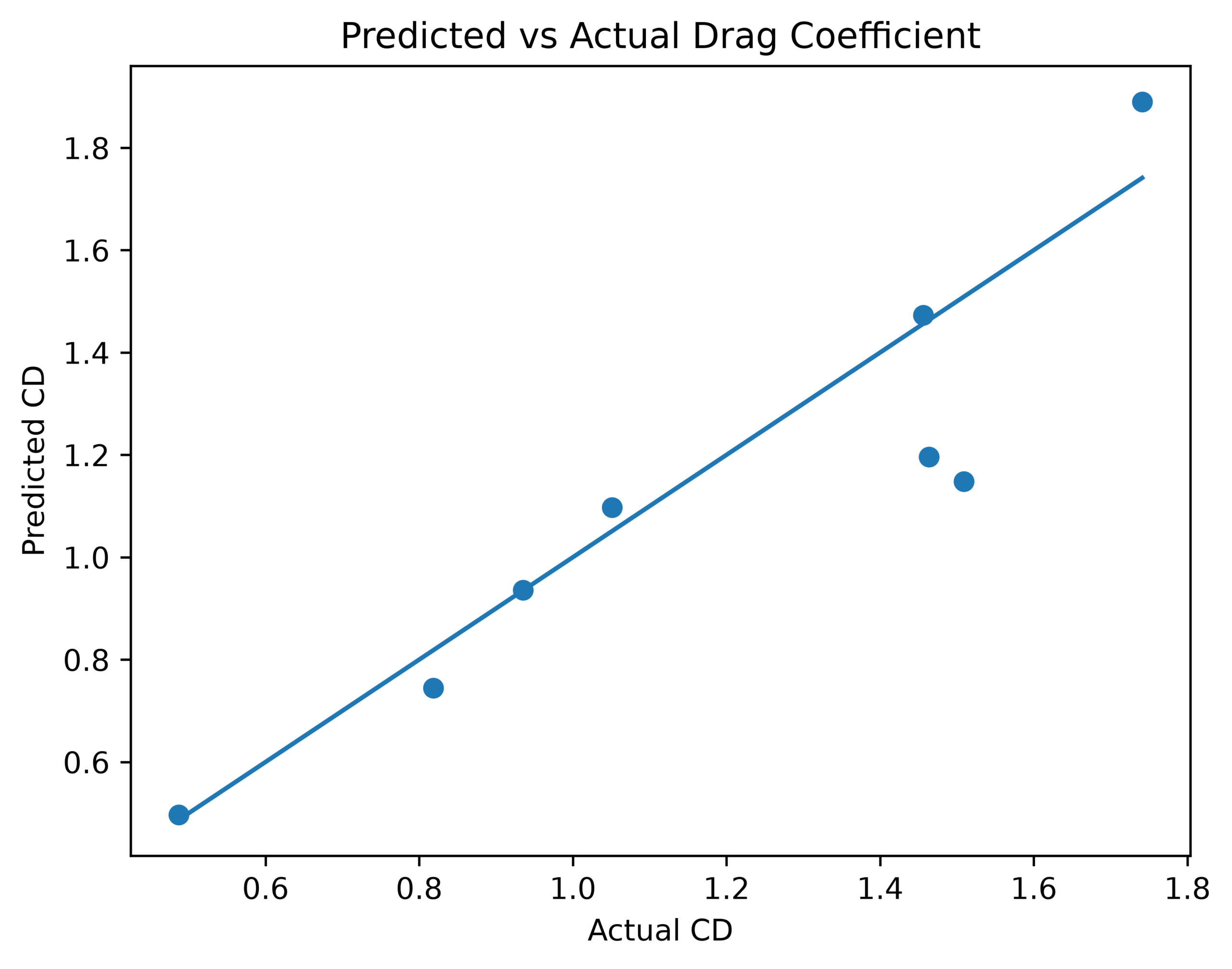
Figure 3 displays the relationship between effective geometry thickness and drag coefficient.

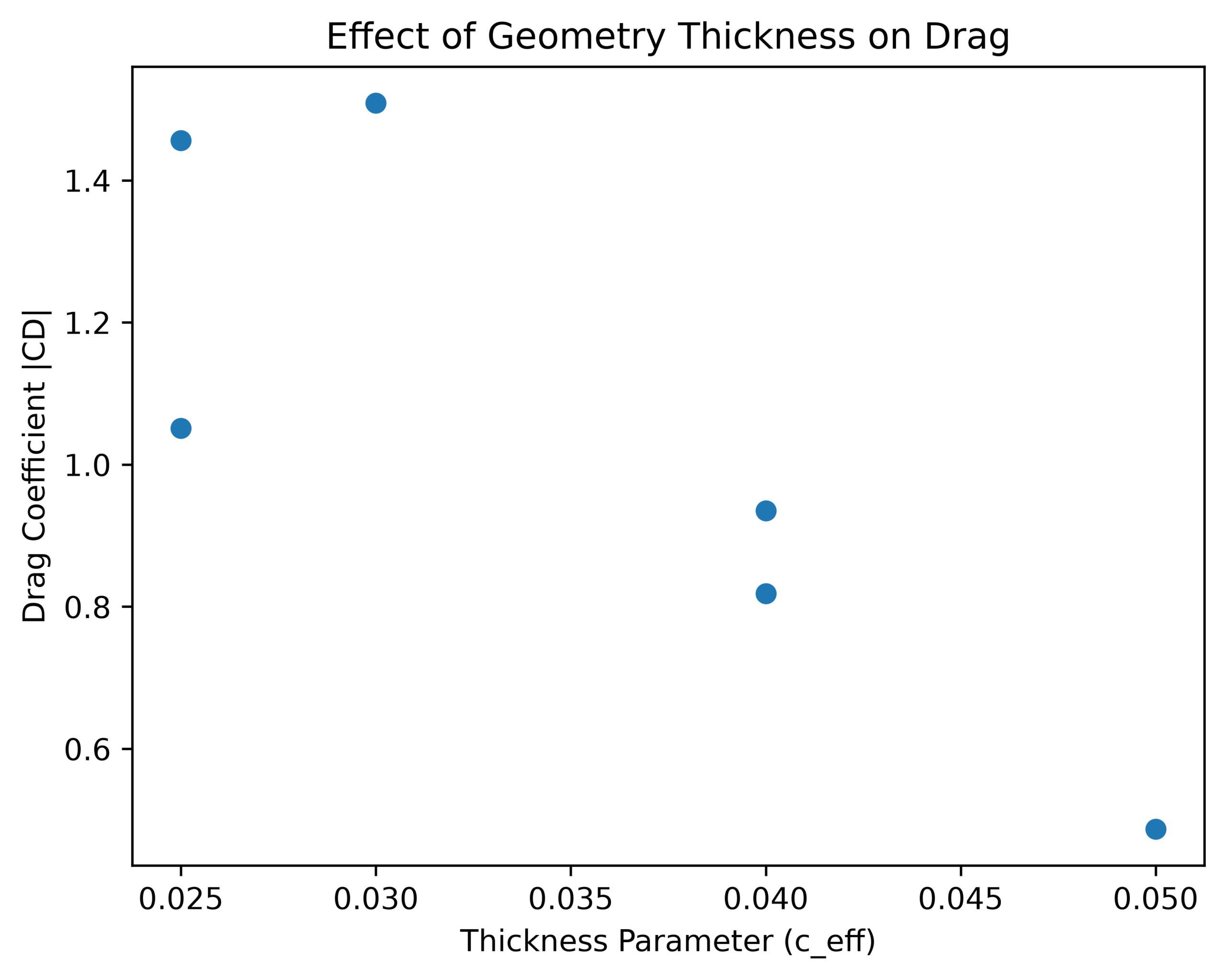
Effective thickness also showed a strong numerical association with drag within the sampled design space. Dividing the 1000 CFD cases into five equally populated bands of showed that the mean increased from 0.827 for to 1.185 for . The corresponding median values increased from 0.865 to 1.216. The intermediate thickness bands exhibited mean values of 1.021, 1.103, and 1.121, respectively. Thus, for the geometries tested, designs with less effective thickness were associated with lower drag magnitudes. The present data does not provide evidence that drag decreased for each ideal middle thickness and increased again for the thinnest design; therefore, there is no proof of a general “moderate” or “extreme” threshold. Regardless, thickness should not be interpreted by itself, as other geometric parameters also had an effect on drag. The dataset was also divided into five equal-count bands based on length and width , in order to verify if any similar trends occurred for other primary dimensions. Length’s association with drag was shown to be non-monotonic. Mean decreased from 1.089 for to a minimum of 0.959 for , before increasing to 1.102 for . Width showed a different pattern: mean remained approximately 1.05–1.12 across the four narrower bands but decreased to 0.856 in the widest band, .

These individual parameter trends show that interactions involving length, width, and effective thickness also affect the observed drag trends, and thickness alone cannot be used to explain drag behavior. These observed bivariate trends and relationships should be considered associations instead of individual drag effects, as the geometric variables were different at the same time frames in the sampled dataset.

These findings support the fact that geometric proportions have a more significant effect on aerodynamic performance than any single design parameter does. For most of the selected validation cases, the surrogate model predictions generally agreed with the patterns found in the CFD results. However, prediction errors increased for geometries approaching or extending beyond the boundaries of the sampled design space, emphasizing that the surrogate model should be used primarily for interpolation within the training distribution rather than extrapolation beyond it.

Table 3 contrasts the geometry that was produced by the corrected surrogate optimization and its CFD evaluation that was run separately.

Parameter	Value
a	0.062535 m
b	0.041690 m
c	0.028000 m
d	0.950000
	0.026600 m
Surrogate-predicted	0.45999
CFD at iteration 1000	-0.39789
CFD convergence status	Oscillatory
Minimum in original dataset	0.44092
Camera constraints satisfied	Yes

Because different housing geometries have different frontal areas, another optimization that minimized drag area, , which is the result of multiplying and , as the main optimization target instead of minimizing the drag coefficient. The rules of the corrected optimization were once again used on the second optimization. The same parameter bounds, effective-thickness definition, aspect-ratio restrictions, and camera-containment constraints were all re-used for the second optimization. The resulting candidate was

with

The predicted value from the surrogate model was . Using the geometry-dependent projected reference area,

the candidate had and a predicted drag-area magnitude of

For comparison, the minimum drag-area magnitude among the original 1000 CFD cases was 0.001671m. As a result, optimization using instead of the drag coefficient alone identified a geometry that had a lower surrogate-predicted drag-area penalty than any of the values in the original dataset.

Parameter	Value
a	0.061675 m
b	0.041117 m
c	0.028000 m
d	0.950000
	0.026600 m
Predicted	0.46130
Predicted	0.003436 m2
Predicted	0.001585 m2
Minimum dataset	0.001671 m2

Discussion

Surrogate modeling was shown to be very useful for identifying meaningful relationships between geometries and aerodynamic performance, with a much lower demand for computation expense than what would be required for running each CFD for every new geometry. Analyzing the 1000 CFD cases in the sampled range indicated that lower drag magnitude mostly resulted from smaller effective thickness. However, since the points on the thickness vs drag plot are not linear, thickness itself cannot explain aerodynamic performance, and length, width, and the resulting geometric proportions must all be evaluated with it. The behavior of the model at the boundary of the parameter space is generally poor. Data-driven models are best at interpolating within regions of the data space that have been well represented within the training data. As one moves away from this well represented region the accuracy of the model can decrease significantly. However, within better-represented regions of the design space, the model can capture useful aerodynamic trends to aid in exploratory design iterations. The accuracy of individual predictions must, however, be interpreted in light of the observed validation errors for that region. A major limitation of unconstrained surrogate-based design for aerodynamic shape optimization has been presented in this work was observed during preliminary optimization attempts. The optimizer entered poorly sampled regions of the design space and produced nonphysical predictions, including negative drag-coefficient values. Since these exploratory runs were not deliberately saved, conclusions on how often negative predictions happened cannot be confirmed. More importantly, the original constrained implementation subsequently produced an apparent optimum at , exactly at the imposed lower rejection threshold, despite the minimum drag magnitude in the 1000-case CFD training dataset being . Since the difference in values was noticeably large, the optimizer was likely exaggerating the more unreliable surrogate predictions near the lower threshold instead of searching for more reliable designs. After evaluating the problem, the optimization procedure was limited to only search within the range that was covered by the CFD training data. The revised search would only consider a geometry if it satisfied all the requirements of the CFD design space. The requirements included bounds on the main four parameters, an effective thickness variable, restrictions on dimensions, an additional camera containment fit of the camera inside the housing.

The corrected optimum had a surrogate-predicted and was subsequently evaluated with CFD, which produced calculated (). Based on these results, geometries should be verified with design constraints and separate CFD evaluation before being applied to draw confident conclusions. The simulations in this study do not represent a real vehicle’s full conditions but nevertheless serve as an efficient way to identify general aerodynamic trends. This is because of the use of a simplified housing model instead of a full automotive mirror design. The study also used simplified laminar CFD modeling as a controlled numerical method to create the original 1000-case CFD dataset. Using these simplified systems made the process of computing the large sample size more practical. Regardless of its efficiency, limitations of this method were found during numerical checks. Varied values would result from the simulations even when the geometry’s CFD run was run for extra iterations. This fluctuation shows that the final iteration’s given drag coefficient is not enough by itself to confirm the CFD solution’s convergence. The fluctuation was expected to decrease as the simulation reached its end, which was discovered when using SST-RANS to compare. Regardless of the decrease in variation, mesh resolution was still shown to be affecting the results. Based on these results, the CFD and surrogate predictions should not be used to provide completely exact values of aerodynamics when applied to a full vehicle design. In order to draw conclusions that can be applied to automotive design, future tests should utilize more advanced systems such as refined near-wall mesh and control, verification of result being unaffected by domain size, time-dependent CFD simulations, and comparison with physical testing. Every CFD case used a one freestream speed of 10m/s, so the resulting dataset only covers one operating condition rather than the range of Reynolds numbers experienced during real operating conditions. Using the characteristic housing dimensions in the present design space, air density near standard atmospheric conditions, and the specified dynamic viscosity of Pas, the Reynolds Numbers corresponding with these are estimated to be —. These flow conditions allow for flow separation to occur, and results can also change depending on transition and turbulence. Given these limitations, the simulation approach should not be interpreted as a full representation of a real automotive mirror’s surrounding airflow, but as a practical method of comparing 1000 geometries. Since every training case used 10 m/s, the neural network is never given data about the change in aerodynamic behavior, meaning assumptions of the surrogate’s predictions being accurate at many different operating speed should not be made. Future CFD datasets should determine whether the observed relationships between geometry and aerodynamic performance exist with different conditions by using multiple different air speeds other than 10 m/s and also utilizing more detailed treatment of turbulence. The reliability of the surrogate model’s predictions is also highest for geometries similar to its training data. The fact that the greater differences between CFD and surrogate predictions came from the geometries near extreme parts of the sampled range also supports the need for caution when using the model’s predictions on designs with less represented training data.

The results of this study provide evidence that machine learning surrogate models can identify aerodynamic drag trends of teardrop-inspired geometries in the sampled design space without being required to run a new CFD simulation for every geometry. While thickness alone couldn’t account for all the drag variation without length, width, and proportions being considered, lower thickness did tend to associate with lower drag magnitude. These results should be considered with the simplified CFD setup and sampled design space used in this study. These results provide understanding of the aerodynamic systems of smaller components, particularly referring to the recently emerging camera-based side mirror systems in automotive designs. With the upcoming trend of traditional side-mirror designs being replaced by more compact teardrop-shaped camera housings, the aerodynamic shapes of the side-mirrors has become increasingly important, as it plays a major role in affecting drag. Besides using surrogate modeling to predict aerodynamic performance, this study also used the SLSQP algorithm to search for improved geometries while ensuring design constraints were being met.

The study also combines neural network prediction, design variable constraints, SLSQP multi-start optimization, and camera-fit requirements, thus creating a complete early-stage design process for aerodynamic geometry optimization.

Since projected frontal areas varied across each geometry, comparing drag coefficient by itself could not fully account for the combined effect of the drag coefficient and frontal area. Because of this, the projected reference area was calculated for every geometry as , and drag area was evaluated as C_dA. Across the original 1000-case dataset, the magnitude of |C_d |A_ref ranged from 0.001671 to 0.008055 m², with a median of 0.004576 m². A separate surrogate optimization using $C_D A$ as the objective produced a predicted minimum of 0.001585 m², which was slightly lower than the lowest value from the original 1000 CFD geometries. This comparison indicates that both front-casing area of mirror and drag coefficient can affect the aerodynamic performance and provides an objective that includes more of the physical size difference between geometries than C_d alone.

Future work using these methods should be done with improved designs and testing parameters on complete vehicle models.

References

1. J. D. Anderson. Fundamentals of Aerodynamics. 5th ed., McGraw-Hill, 2010. [↩]
2. H. K. Versteeg, W. Malalasekera. An Introduction to Computational Fluid Dynamics: The Finite Volume Method. 2nd ed., Pearson Education, 2007. [↩]
3. A. Forrester, A. Sóbester, A. Keane. Engineering Design via Surrogate Modelling: A Practical Guide. Wiley, 2008. [↩]
4. M. Zaareer, A. H. Mourad. Effect of vehicle side mirror base position on aerodynamic forces and acoustics. Alexandria Engineering Journal. Vol. 61, pg. 1437–1448, 2022, https://doi.org/10.1016/j.aej.2021.06.049. [↩]
5. M. S. Rahman, M. A. S. Sakib, K. N. Rimi, M. M. Hasan, M. Islam, T. Mahbub. Experimental characterization and adjoint optimization of side-view mirror geometry for aerodynamic drag reduction. Discover Vehicles. Vol. 2, Article 23, 2026. [↩]
6. S. Sankarapandian, S. S. Rajasekaran, N. N. A. Riffai, R. R. Subburaj. Aerodynamic drag reduction of a passenger car through shape optimization of outside rear view mirrors. Proceedings of the Institution of Mechanical Engineers, Part D: Journal of Automobile Engineering. 2026, https://doi.org/10.1177/09544070261421268. [↩]
7. J. Ye, M. Xu, P. Xing, Y. Cheng, D. Meng, Y. Tang, M. Zhu. Investigation of aerodynamic noise reduction of exterior side view mirror based on bionic shark fin structure. Applied Acoustics. Vol. 182, 108188, 2021, https://doi.org/10.1016/j.apacoust.2021.108188. [↩]
8. W. Fu, Y. Li. Experimental study on a generic side-view mirror with slotted cylindrical foot. Journal of Applied Fluid Mechanics. Vol. 16, pg. 363–374, 2023, https://doi.org/10.47176/jafm.16.02.1424. [↩]
9. M. N. Zaareer, A. H. I. Mourad, T. Darabseh, K. Abdullah, M. S. A. ElSayed. Aeroacoustics wind noise optimization for vehicle’s side mirror base. International Journal of Thermofluids. Vol. 18, pg. 100332, 2023, https://doi.org/10.1016/j.ijft.2023.100332. [↩]
10. K. K. Chode, H. Viswanathan, K. Chow, H. Reese. Investigating the aerodynamic drag and noise characteristics of a standard squareback vehicle with inclined side-view mirror configurations using a hybrid computational aeroacoustics (CAA) approach. Physics of Fluids. Vol. 35, pg. 075148, 2023, https://doi.org/10.1063/5.0156111. [↩]
11. P. Uhl, A. Schell, R. Ewert, J. Delfs. Stochastic noise sources for computational aeroacoustics of a vehicle side mirror. SAE International Journal of Passenger Vehicle Systems. Vol. 17, pg. 65–80, 2024, https://doi.org/10.4271/15-17-01-0005. [↩]
12. O. Yemenici, M. Vatansever Ensarioğlu. Experimental and numerical investigation of aerodynamics of optimum side-view mirror geometries. Applied Sciences. Vol. 15, pg. 10731, 2025, https://doi.org/10.3390/app151910731. [↩]
13. X. Zhang, F. Xie, T. Ji, Z. Zhu, Y. Zheng. Multi-fidelity deep neural network surrogate model for aerodynamic shape optimization. Computer Methods in Applied Mechanics and Engineering. Vol. 373, 113485, 2021, https://doi.org/10.1016/j.cma.2020.113485. [↩]
14. P. Liao, W. Song, P. Du, H. Zhao. Multi-fidelity convolutional neural network surrogate model for aerodynamic optimization based on transfer learning. Physics of Fluids. Vol. 33, 127121, 2021, https://doi.org/10.1063/5.0076538. [↩]
15. C. Duru, H. Alemdar, O. U. Baran. A deep learning approach for the transonic flow field predictions around airfoils. Computers & Fluids. Vol. 236, 105312, 2022, https://doi.org/10.1016/j.compfluid.2022.105312. [↩]
16. Z. Deng, J. Wang, H. Liu, H. Xie, B. Li, M. Zhang, T. Jia, Y. Zhang, Z. Wang, B. Dong. Prediction of transonic flow over supercritical airfoils using geometric-encoding and deep-learning strategies. Physics of Fluids. Vol. 35, 075146, 2023, https://doi.org/10.1063/5.0155383. [↩]
17. Z. Wang, X. Liu, J. Yu, H. Wu, H. Lyu. A general deep transfer learning framework for predicting the flow field of airfoils with small data. Computers & Fluids. Vol. 251, 105738, 2023, https://doi.org/10.1016/j.compfluid.2022.105738. [↩]
18. Q. Du, T. Liu, L. Yang, L. Li, D. Zhang, Y. Xie. Airfoil design and surrogate modeling for performance prediction based on deep learning method. Physics of Fluids. Vol. 34, 015111, 2022, https://doi.org/10.1063/5.0075784. [↩]
19. A. Glaws, R. N. King, G. Vijayakumar, S. Ananthan. Invertible neural networks for airfoil design. AIAA Journal. 2022, https://doi.org/10.2514/1.J060866. [↩]
20. J. Li, M. Zhang, J. R. R. A. Martins, C. Shu. Efficient aerodynamic shape optimization with deep-learning-based geometric filtering. AIAA Journal. 2020, https://doi.org/10.2514/1.J059254. [↩]
21. Y. Feng, L. Lv, X. Yan, B. Ai, T. Liu. A gradient-improved sampling plan for surrogate-based aerodynamic shape optimization. Physics of Fluids. Vol. 36, 086115, 2024. [↩]
22. B. Eiximeno, A. Miró, I. Rodríguez, O. Lehmkuhl. Toward the usage of deep learning surrogate models in ground vehicle aerodynamics. Mathematics. Vol. 12, pg. 998, 2024, https://doi.org/10.3390/math12070998. [↩]
23. K. Shukla, V. Oommen, A. Peyvan, M. Penwarden, N. Plewacki, L. Bravo, A. Ghoshal, R. M. Kirby, G. E. Karniadakis. Deep neural operators as accurate surrogates for shape optimization. Engineering Applications of Artificial Intelligence. Vol. 129, pg. 107615, 2024, https://doi.org/10.1016/j.engappai.2023.107615. [↩]
24. D. Pereira, F. Afonso, F. Lau. End-to-end deep-learning-based surrogate modeling for supersonic airfoil shape optimization. Aerospace. Vol. 12, pg. 389, 2025, https://doi.org/10.3390/aerospace12050389. [↩]
25. S. Wang, Q. Xu, N. Wei. Airfoil aerodynamic optimization design using ensemble learning surrogate model. Journal of Aerospace Engineering. Vol. 37, 2024, https://doi.org/10.1061/JAEEEZ.ASENG-5410. [↩]
26. J. Jabón, S. Corbera, R. Álvarez, R. Barea. Aerodynamic shape optimization using graph variational autoencoders and genetic algorithms. Structural and Multidisciplinary Optimization. Vol. 67, Article 32, 2024, https://doi.org/10.1007/s00158-024-03771-5. [↩]
27. Z. Zhang, Y. Ao, S. Li, G. X. Gu. An adaptive machine learning-based optimization method in the aerodynamic analysis of a finite wing under various cruise conditions. Theoretical and Applied Mechanics Letters. Vol. 14, pg. 100489, 2024, https://doi.org/10.1016/j.taml.2023.100489. [↩]
28. C. M. Aye, K. Wansaseub, S. Kumar, G. G. Tejani, S. Bureerat, A. R. Yildiz, N. Pholdee. Airfoil shape optimisation using a multi-fidelity surrogate-assisted metaheuristic with a new multi-objective infill sampling technique. Computer Modeling in Engineering & Sciences. Vol. 137, pg. 2111–2128, 2023, https://doi.org/10.32604/cmes.2023.028632. [↩]
29. J. Parekh, P. Bekemeyer, S. Helm, D. G. François, C. Grabe. Surrogate based design space exploration and exploitation for an efficient airfoil optimization under uncertainties using transition models. Aerospace Science and Technology. Vol. 154, pg. 109532, 2024, https://doi.org/10.1016/j.ast.2024.109532. [↩]
30. T. D. Economon, F. Palacios, S. R. Copeland, T. W. Lukaczyk, J. J. Alonso. SU2: An open-source suite for multiphysics simulation and design. AIAA Journal. Vol. 54, pg. 828–846, 2016, https://doi.org/10.2514/1.J053813. [↩]
31. A. Paszke, S. Gross, F. Massa, A. Lerer, J. Bradbury, G. Chanan, T. Killeen, Z. Lin, N. Gimelshein, L. Antiga, A. Desmaison, A. Köpf, E. Yang, Z. DeVito, M. Raison, A. Tejani, S. Chilamkurthy, B. Steiner, L. Fang, J. Bai, S. Chintala. PyTorch: An imperative style, high-performance deep learning library. Advances in Neural Information Processing Systems. Vol. 32, pg. 8024–8035, 2019. [↩]
32. V. Nair, G. E. Hinton. Rectified linear units improve restricted Boltzmann machines. Proceedings of the 27th International Conference on Machine Learning. pg. 807–814, 2010. [↩]
33. D. P. Kingma, J. Ba. Adam: A method for stochastic optimization. International Conference on Learning Representations. 2015. [↩]