Empirical Evaluation of Stochastic Rule Layers in a Partially Observable Battleship Game

Abstract

Battleship is a partially observable search game in which players infer hidden ship locations through sequential hit-or-miss observations. This study uses Battleship as a stochastic hidden-state framework for testing how added hidden transition rules affect decision-making under partial observability. Because the environment keeps the visible game rules interpretable while varying hidden transitions, policies, board size, and measurement probability, it provides a testbed rather than only a new Battleship variant. The implemented model is a classical stochastic simulation with quantum-circuit-sampled transition variables: board state, ship placement, legal moves, observations, hit/sunk logic, and terminal outcomes remain classical, while selected hidden rule transitions are resolved through Qiskit-simulated circuit measurements and mapped back to classical rule outcomes. The classical baseline, L0, was compared with three cumulative modified levels: attack-type-dependent vulnerability, L1; branch-based hidden placement, L2; and cross-grid correlated damage, L3. All levels were evaluated as two-player games using paired layout packets, both start orders, and automated policies: random targeting, checkerboard search with local follow-up, belief-state probability mapping, and greedy maximum-probability targeting. Experiments covered 5×5 and 10×10 boards, with p = 0.50 as the main measurement-probability condition and p = 0.25 and p = 0.75 as sensitivity conditions. The final run contained 160 configurations and 6,400 completed games. Results showed configuration-specific effects of rule level, policy, board size, and measurement probability, without showing quantum advantage or universal improvement over the classical baseline.

Keywords: Battleship, partially observable decision-making, stochastic search, hidden-state inference, POMDP, circuit-sampled stochastic transitions, belief-state policy, classical stochastic game.

Introduction

Many decision-making problems require an agent to act while the true state of the environment is only partly known. Stochastic games model sequential decisions in which outcomes depend on both player actions and probabilistic transitions, while partially observable Markov decision processes, or POMDPs, model settings in which an agent must choose actions using observations rather than complete knowledge of the state^1,2,3,4. In these environments, performance depends not only on the underlying rules, but also on how effectively an agent updates its beliefs after each observation and uses those beliefs to choose future actions^5,6,7,8. Battleship provides a compact example of this structure. The true ship locations are hidden, each move produces limited feedback, and the player must use a sequence of hit-or-miss observations to infer where future shots are most likely to be useful.

Prior work on POMDPs has shown that exact planning under partial observability is difficult because the agent must reason over belief states rather than directly observed states^4,5. Approximate methods such as point-based value iteration, randomized point-based updates, and Monte Carlo planning have been developed to make belief-space planning more practical in larger domains^6,7,8,9. In game-playing research, heuristic search and sampling-based methods have also been used to select actions in large decision spaces, where evaluating every possible continuation is computationally expensive^10,11,12. However, the purpose of the present study is not to solve Battleship optimally. Instead, Battleship is used as a controlled hidden-state search environment in which defined policies are compared under progressively modified rules.

Battleship-related computational work has treated the game and its puzzle variants as search, inference, and algorithmic problems¹³. Sevenster showed that the solitaire Battleships puzzle can be formulated as a decision problem, linking Battleship-style reasoning to computational complexity¹³. More generally, Battleship strategies often rely on reducing the set of possible legal ship placements after misses and hits, then targeting cells that are consistent with many remaining placements. This connects naturally to belief-state and probability-map approaches, where observations are used to update a distribution over possible hidden configurations^5,6,7,13. The present study builds on this idea, but changes the question being asked. Rather than only asking which policy finds ships fastest in the standard game, it asks how added hidden rule transitions change search efficiency, terminal outcomes, and fairness-related measures under the same defined policies. The contribution of this study is therefore not a new optimal Battleship solver, but an experimentally controlled stochastic hidden-state environment for testing how added hidden transitions affect search efficiency, terminal outcomes, and fairness-related measures under partial observability.

Recent reviews of POMDP planning and robotics describe the continuing difficulty of choosing actions from incomplete observations and maintaining useful belief representations in large state spaces^14,15. Recent studies have also examined POMDP planning under object composition uncertainty in robotic manipulation¹⁶, probabilistic decision-making for robotic path planning¹⁷, collaborative human-autonomy semantic sensing¹⁸, human-robot interaction¹⁹, and sequential decision-making under uncertainty²⁰. These studies demonstrate different forms of belief updating and information gathering, but their results are tied to their own state, action, observation, and objective definitions. Recent algorithmic work has reduced online planning cost through hybrid parallelization, multilevel Monte Carlo simulation, learned state-variable relationships, non-linearity-guided simplification, and adaptive Voronoi discretization^{21,22,23,24,25}. Learning-based and Bayesian-optimized planning studies provide additional examples of approximation for large belief spaces^26,27. The cited literature addresses POMDP planning and Battleship-style algorithmic complexity, but it does not evaluate the specific cumulative L0–L3 rule-layer design used here^13,28. This study addresses that narrower gap by holding layout packets, start orders, board conditions, automated policies, and outcome definitions fixed while changing the hidden rule transitions across L0–L3.

The study is also related to pursuit-evasion and search games, where one agent attempts to locate, track, or capture a hidden or moving target^29,30,31,32. Recent primary studies examine differential-drive dynamics, three-player pursuit-evasion, and multi-pursuer systems^33,34,35.

Other work investigates neural-network controllers, multi-UAV reinforcement-learning schemes, agent team formation, and optimal strategies for three pursuers^36,37,38,39. The diversity of these models shows that pursuit-evasion findings depend on the specified dynamics, information structure, and capture criterion. Accordingly, the present study holds policies, layout packets, start orders, and outcome definitions fixed when comparing rule levels. Battleship differs from many pursuit-evasion models because the targets are fixed ship segments rather than moving agents, but the problem is still partial information: the searcher must choose actions without directly observing the hidden state. This makes Battleship useful for studying how rule changes affect hidden-state search without requiring a large physical environment or complex movement model.

The model in this study is classical at the game-state level, with quantum-circuit measurements used only to resolve selected stochastic transition variables. Formal quantum games use quantum states, quantum operations, strategy spaces, and measurement rules to define game structure and outcomes^{40,41,42,43,44}. Hybrid quantum-classical algorithms instead combine circuit measurements with classical processing, but they do not automatically make every part of the surrounding system quantum^{45,46,47,48,49}. Recent primary studies use hybrid or near-term quantum workflows for quantum-assisted Monte Carlo, photonic parameter estimation, electron-phonon simulation, entanglement estimation, and information-sharing variational optimization^{50,51,52,53,54}. Other recent studies apply related workflows to protein folding, hybrid quantum-classical machine learning, NISQ complexity analysis, and algorithmic measurement^55,56,57,58.These studies support the distinction between a hybrid procedure and a fully quantum game; they do not establish quantum advantage for the present simulation. In the present work, the Battleship board, ship positions, legal moves, observations, hit/sunk logic, and terminal outcomes remain classical. The quantum-circuit-assisted component consists of selected hidden rule transitions that are resolved using Qiskit-simulated circuit measurements, and the measured outputs are then mapped immediately into classical game-state updates. Therefore, the study does not claim quantum advantage, physical entanglement of ships, or Hilbert-space evolution of the board. The circuit measurements are used only to resolve specified stochastic transitions inside an otherwise classical partially observable game.

The classical baseline, L0, is compared with three modified rule levels. L1 adds attack-type-dependent vulnerability, L2 adds branch-based hidden placement, and L3 adds cross-grid correlated damage. These rule layers are implemented progressively, so a higher level contains the features of the lower levels plus its own added feature. The detailed transition rules, circuit-measurement mapping, paired-layout design, and recorded outcomes are described in Materials and Methods.

This study therefore investigates how stochastic rule layers in Battleship affect search efficiency, terminal outcomes, and fairness-related measures under different policies, board sizes, and measurement-probability conditions.

Materials and Methods

Experimental overview

The experiment tested a two-player Battleship environment under four rule levels: L0, L1, L2, and L3. Each game used two players. Player 1 and Player 2 each had one board and the same fleet of three ships: S1 of length 2, S2 of length 3, and S3 of length 4. Players alternated turns, and each turn consisted of one legal shot at the opponent’s board. When required by the rule level, the shot also included an attack type. A game ended when one player’s fleet was fully sunk or when both fleets were fully sunk in the same terminal event. Terminal outcomes were recorded as Player 1 win, Player 2 win, or draw. All rule levels were evaluated using the same two-player structure. This was necessary because terminal outcomes, starting-player effects, and fairness-related measures cannot be compared consistently if some levels are simulated as one-player searches and other levels are simulated as two-player games.

Rule levels

Each higher level retained the earlier rule layers and added one new mechanic. Thus, L2 included the L1 attack-vulnerability rule, and L3 included both L1 and L2 plus its correlated-damage rule. Representative rule-level walkthroughs are provided in Supplementary File S1.

L0: classical baseline. L0 used fixed ship placement and deterministic damage. At the start of a trial, each ship had one placement on the board. A legal shot at an occupied coordinate damaged the targeted ship segment, while a shot at an empty coordinate was recorded as a miss. L0 therefore provided the baseline for measuring how the added stochastic rule layers changed gameplay.

L1: circuit-sampled vulnerability. L1 added uncertainty after a player selected a coordinate. In L1, a shot at an occupied coordinate did not automatically cause damage. The shot also depended on the selected attack type and a hidden vulnerability outcome. A circuit-measured transition determined whether the selected attack type could damage the occupied segment. If the measured outcome allowed damage, the occupied segment was marked as damaged; if not, the shot produced no damage even though the coordinate was occupied. From the perspective of a player’s observed feedback, a no-damage outcome could therefore reflect either an empty coordinate or an occupied coordinate whose vulnerability outcome did not permit damage. In the implemented experiment, attack type was not a separate strategic choice made by the targeting policies. Each policy selected the target coordinate. After coordinate selection, the shared shot routine assigned and recorded one of two attack-type labels, bomb or torpedo, using the same rule across all policies, players, board sizes, and start orders. The attack type did not change the measurement-probability parameter p. Instead, p controlled the probability that the vulnerability bit equalled 1 for the selected attack event. If the targeted coordinate was occupied and the measured vulnerability bit was 1, damage was applied to that coordinate. If the targeted coordinate was occupied and the measured vulnerability bit was 0, no damage was applied. If the targeted coordinate was empty, no damage was applied regardless of the vulnerability bit. Thus, the circuit-sampled vulnerability rule affected the mapping from an occupied target to damage, while the policies remained comparable because the same attack-type assignment and vulnerability rule was used for every policy.

L2: branch-based hidden placement. L2 added uncertainty about which placement of a ship was active. In the final experiment, each player had branch candidates for all three ships, S1, S2, and S3. For each ship on each player board, the paired layout packet stored two candidate classical placement branches before resolution. These two branches were distinct and did not overlap for the same ship, so a coordinate could not belong to both Branch A and Branch B for that ship in the corrected layout banks. Branch resolution was performed separately for each ship on each player board when a shot required the game to determine whether the targeted coordinate belonged to one of that ship’s retained candidate branches. The measured branch-selection bit selected the active branch for that ship. After branch resolution, the selected branch remained fixed for that ship for the rest of the game, and the inactive branch was removed from active gameplay. Later hit, damage, and sunk-ship logic for that ship used only the selected active branch. This rule uses a branch-selection analogy only in the limited sense that two stored classical alternatives are retained before a circuit-sampled rule event selects one active branch.

L3: cross-grid correlated damage. L3 retained the L1 attack-vulnerability rule and the L2 branch-selection rule, then added predefined correlated-link squares between ship segments on the two players’ boards. When the linked-damage rule was triggered, correlated measurement bits were mapped onto the stored linked coordinates. Any resulting linked damage was then applied as a classical board update during the same move. Because this rule could damage a directly targeted segment and a linked segment in the same turn, L3 could change terminal outcomes and could also create a draw if both fleets were completed in the same terminal event. Direct target damage and correlated damage were therefore recorded separately. L3 was treated as a correlation-based rule analogy in this limited sense; the ship segments themselves were not represented as quantum-entangled subsystems.

Hybrid quantum-classical transition

The game was implemented as a classical partially observable stochastic game with selected hidden transition variables resolved through Qiskit-simulated circuit measurements. The board, ship coordinates, legal moves, player actions, observations, hit logic, sunk-ship logic, and terminal outcomes remained classical. The quantum-circuit-assisted component was limited to sampling selected hidden rule transitions and immediately mapping the measured outputs back into classical rule outcomes. This framing follows the distinction between hybrid quantum-classical procedures and fully quantum game models: measured circuit outputs can be used inside a classical computation without making the full system a quantum state^45,46,59. The circuit measurements were run through Qiskit, and the final manuscript experiment used the Qiskit 2.3.0 statevector executor⁶⁰.

Formally, the transition from a current classical game state s to a next classical game state s′ after action a can be represented as:

T(s′ | s,a) = ∑_m P_θ(m) 1[s′ = f(s,a,m)]

Here, m denotes the measured circuit output, P_θ(m) is the measurement probability induced by the circuit parameter θ, and f(s,a,m) is the deterministic classical update rule that maps the current state s, selected action a, and measured output m to the next classical state.

The rule-layer updates were represented using the following binary state-update notation. These equations describe the implemented rule logic. Let x be the targeted coordinate. Let O(x) = 1 if x contains an active ship segment under the currently active placement, and O(x) = 0 otherwise. Let D(x) = 1 if the move produces direct damage at x, and D(x) = 0 otherwise. For L0, damage is deterministic because a shot damages the target if and only if the coordinate is occupied:

D_L0(x) = O(x)

For L1, a measured vulnerability bit V determines whether an occupied coordinate is actually damaged:

D_L1(x) = O(x)V,    V ∈ {0,1}

This means an empty coordinate remains a miss, while an occupied coordinate causes damage only when the measured vulnerability outcome permits it.

For L2, let P0 and P1 be the two stored candidate placement branches, and let B be the measured branch-selection bit. After branch resolution, the active branch is:

P_active = P_B,    B ∈ {0,1}

After the active branch is selected, occupancy is evaluated on that selected branch. Because L2 includes the L1 vulnerability rule, the direct-damage update after branch resolution can be written as:

D_L2(x) = O_PB(x)V

For L3, direct target damage and correlated linked-coordinate damage are kept separate. Let y be a predefined linked coordinate and let C be the mapped correlated measurement outcome used by the linked-damage rule. The direct and correlated components are:

D_direct(x) = O_PB(x)V

D_correlated(y,C) = L(y)C

where L(y) = 1 when y is an eligible linked coordinate for that move and L(y) = 0 otherwise. The total L3 recorded damage event count can therefore be summarized as:

     D_L3(x,y) = D_direct(x) + D_correlated(y,C)

Here, D_L3 is a count of recorded damage events in that move. It can include direct target damage, correlated linked damage, both, or neither. This matters because correlated damage is not the same as ordinary direct-hit efficiency.

For L1 and L2, one-qubit circuit measurements were used to resolve the attack-vulnerability and branch-selection transitions. In each case, the measured bit was immediately mapped to a classical rule outcome. For probability-controlled one-qubit transitions, the probability of measuring 1 was represented as:

P(m = 1) = p = sin²(θ/2),    θ = 2 arcsin(√p)

Here, p denotes the circuit-measurement probability, or the probability that the measured bit equals 1 for the relevant transition. The main experiment used p = 0.50 as a neutral maximum-uncertainty baseline because neither stochastic outcome is favoured. The p = 0.25 and p = 0.75 conditions test whether observed effects are specific to that neutral setting or persist when the hidden transition is biased toward failure or success. The corresponding rotation settings were θ = π/3 for p = 0.25, θ = π/2 for p = 0.50, and θ = 2π/3 for p = 0.75, following p = sin²(θ/2).

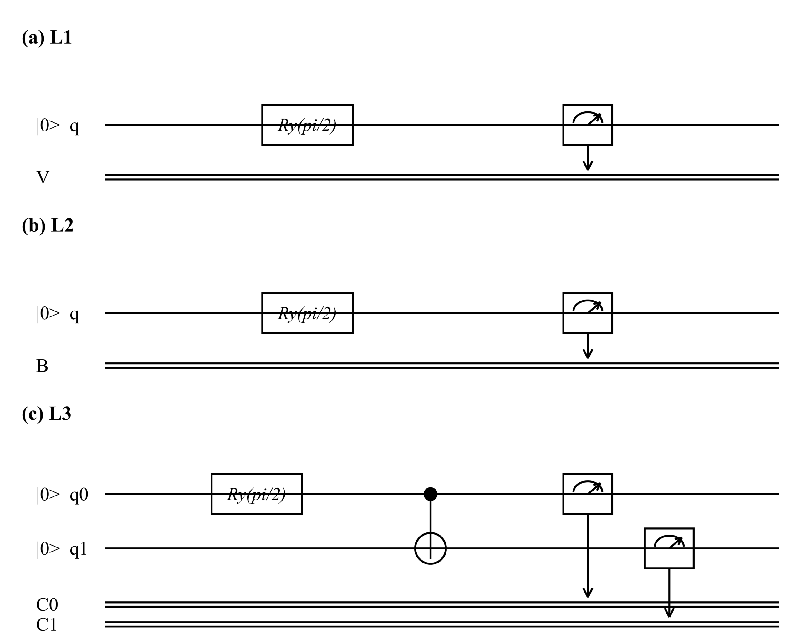
As shown in Figure 1, the circuits are used to generate measured outputs for the selected hidden rule transitions. In Figure 1(a), qubit q is initialized as |0⟩, rotated by R_y(θ), and measured to define the L1 vulnerability variable V. In Figure 1(b), the same one-qubit measurement structure defines the L2 branch-selection variable B. In Figure 1(c), qubits q₀ and q₁ are initialized as |00⟩; after R_y(θ) on q₀ and a controlled-X operation, the measured outputs C₀ and C₁ are mapped to predefined linked-damage outcomes for L3. The labels q, q₀, and q₁ denote quantum bits, while V, B, C₀, and C₁ denote classical measurement-derived rule variables. In all three cases, the measured outputs are immediately converted into classical game-state updates, so the Battleship board, ship positions, legal moves, observations, damage logic, and terminal outcomes remain classical.

For L3, a two-qubit correlated circuit was used to generate correlated measurement bits for the linked-damage rule; these bits were mapped to predefined classical linked coordinates and were not treated as a quantum board state. In L3 sensitivity trials, the measurement-probability setting applied to the L1 and L2 circuit-measured transitions inherited within L3, while the L3 correlated-damage circuit was kept as the linked-damage rule and evaluated separately through the L3 direct/correlated damage measures.

Paired layout packets

To reduce layout confounding, each board size used a fixed bank of 40 paired layout packets. A layout packet was the complete stored setup for a trial_id. Each packet contained seed information, Player 1’s base fleet layout, Player 2’s base fleet layout, branch candidates for L2 and L3, and correlated-link candidates for L3. The same trial_id packet was reused across all rule levels, policies, start orders, and measurement-probability conditions. For L0 and L1, the base Player 1 and Player 2 layouts were used directly. For L2 and L3, the same packet also supplied the retained branch candidates. For L3, the same packet additionally supplied correlated-link candidates. Pairing did not mean that L2 or L3 was forced to realize the same final branch as L0. The realized branch and linked-damage outcome remained part of the rule level being evaluated. Pairing meant that the starting layout packet, branch candidates, link candidates, and seeds were controlled across conditions. The corrected layout banks contained no duplicate branch pairs. Therefore, for each branch-based ship, Branch A and Branch B were distinct candidate placements. Representative paired-layout, branch-resolution, and linked-damage visualizations for both board sizes are provided in the project repository listed in Appendix A.

Board-size conditions

Two board sizes were tested: 5×5 and 10×10. Both board sizes used the same three ships of lengths 2, 3, and 4, for a total of nine occupied ship cells per player. The 5×5 board therefore had a ship density of 36%, while the 10×10 board had a ship density of 9%. The 10×10 condition was included to test whether the observed effects changed when the same fleet was placed on a larger and lower-density board. Therefore, comparisons between 5×5 and 10×10 conditions should be interpreted as board-size/ship-density comparisons rather than pure board-size effects.

Search policies

In each configuration, Player 1 and Player 2 were implemented as automated policy-controlled agents using the same assigned targeting policy. Four policies were evaluated so that the rule layers could be tested under unstructured search, structured local search, explicit belief updating, and a stronger probability-based baseline.

Random targeting. The random policy selected legal target coordinates without using parity search, probability maps, or local follow-up after a hit. It provided an unstructured baseline for showing what happens when players do not use observations to guide later shots.

Checkerboard search with local follow-up. The checkerboard policy used alternating-square search during the search phase. Because every ship in the experiment had length at least 2, each legal ship placement had to intersect at least one square of a parity-style search pattern. After a hit, the policy switched to adjacent-square follow-up to identify the ship’s orientation and complete destruction of the ship. Once the ship was sunk, the policy returned to checkerboard search. This policy represented a simple structured Battleship heuristic rather than an optimal planner.

Belief-state probability mapping. The belief-state policy maintained a probability distribution over possible hidden board states and updated that distribution after observations. This follows the standard belief-state approach used in partially observable decision problems^2,4,5. A possible state was constrained by ship lengths, board boundaries, previous misses, confirmed hits, unresolved or resolved branch choices, and rule-level-specific conditions. After each observation, impossible states were removed or downweighted, and the remaining distribution was normalized. Coordinates were then scored by summing the posterior probability assigned to states in which the coordinate contained an active or still-possible ship segment. The policy selected the highest-scoring legal coordinate, with deterministic tie handling.

Greedy maximum-probability targeting. The greedy policy served as a probability-based baseline. At each turn, it selected the legal coordinate with the highest current placement-probability score under the available information. It did not simulate future turns, evaluate long-horizon consequences, or claim optimal play. It was included to test whether a simple strongest-current-cell rule could explain the results without relying on a fuller belief-state policy. Unlike the belief-state policy, the greedy policy did not maintain a full normalized posterior over hidden rule states; it used the current placement-probability score as a simpler maximum-probability baseline.

Belief-policy validation

The belief-state policy was validated before the final runs because the experiment depends on the policy updating hidden-state possibilities correctly^2,4,5. The validation checks confirmed that the initial belief distribution normalized to 1, that misses removed impossible states, that branch-resolution updates matched the selected branch, and that the selected target matched the highest-scoring legal coordinate. In the validation case with tied highest-scoring coordinates, the tie was resolved lexicographically. These checks were used to verify that the belief-state policy updated and selected targets according to the implemented rule logic. The belief-state policy validation output is provided in Supplementary File S2, and all validation checks had passed before the final manuscript run.

Experimental design

For each board size, policy, rule level, start order, and applicable measurement-probability condition, 40 trials were completed. Both start orders were tested: Player 1 starts and Player 2 starts. This allowed terminal outcomes and starting-player effects to be evaluated without fixing one player as the permanent first mover. In summary tables that combine both start orders, each board-size, policy, rule-level, and probability condition therefore contains 80 completed games. Across the full main and sensitivity design, the final run contained 160 configurations and 6,400 completed two-player games. All trials were two-player. L0 was recorded only as the classical baseline and was not treated as measurement-probability-dependent because it had no circuit-measured transition. Detailed experiment verification outputs, belief-policy validation checks, full summary tables, and the raw-data file inventory are provided in Supplementary File S2. An online demonstration version of the game was also produced to show the implemented rule layers in an interactive format. The demonstration version and the project repository are listed in Appendix A. The repository includes the raw trial logs, summary CSV files, paired layout banks, experiment manifest, belief-policy validation output, methodology notes, and representative layout visualizations used to support the manuscript analysis. The complete trace-run output directory includes raw trial logs, summary CSVs, L3 decomposition values, an experiment manifest, SHA256 hashes, and manuscript table exports, enabling recomputation of every reported table value from a single source of truth.

Outcome measures

Search efficiency was evaluated primarily using the logged terminal_turns value, reported in the tables as mean terminal turns. In the experiment logs, terminal_turns is the game-level terminal count at which the completed two-player game reached a Player 1 win, Player 2 win, or draw. This value was analyzed per completed game and was not calculated by summing Player 1 and Player 2 shot counts. Player-level shot counts were recorded separately as Player 1 shots and Player 2 shots and were used for L3 hit-rate denominators. Lower terminal move counts indicated faster game completion under the tested rule level and policy. Terminal outcomes were evaluated using Player 1 wins, Player 2 wins, and draws. At the same time, hit-related measures were used to distinguish between L3’s direct and correlated damage. Fairness-related analysis used starting-player win rate, win-rate disparity, draw rate, and mirrored-start outcome comparison. Win-rate disparity was calculated as |P1 wins − P2 wins| / n, where n is the total number of completed games in that condition, including draws. Draw rate was calculated as draws / n. Mirrored-start parity measured how often start-order outcomes matched after reversing the first mover. Fairness-related metrics were treated as secondary outcome measures rather than the primary performance criterion. They were included because the experiment is a two-player terminal game in which start order, player identity, and L3 draw events could affect interpretation of terminal outcomes separately from search efficiency. First-hit timing was recorded where available but was not used as the main fairness measure. For L3, direct damage and correlated damage were evaluated separately because a correlated-damage event is not the same as an ordinary direct hit by the selected coordinate. L3-specific analysis therefore distinguished direct target hits, additional correlated-damage events, sunk-ship events, and whether correlated damage contributed to the terminal event.

Statistical analysis

Summary statistics were calculated from the trial logs. The trial, defined as one completed two-player game, was the unit of analysis. For each condition, the analysis computed mean terminal-turn count, sample standard deviation, and 95% confidence interval; the main manuscript tables report mean ± 95% CI. Confidence intervals were calculated as mean ± 1.96 × s/√n, where s is the sample standard deviation and n is the number of completed games in that condition. For summary tables that combine both start orders, n = 80 completed games for each board-size, policy, rule-level, and measurement-probability condition. Standard deviations and confidence intervals were calculated over the logged terminal_turns value per completed game, not over per-player shot counts or player-level shot events.

Modified levels were compared against the L0 baseline using trial_id- and start_order-matched differences. This comparison was used because the same layout packet was reused across rule levels.

For each comparison, the paired difference was calculated as:

                                                  paired difference (Δ) = outcome(Lk) − outcome(L0)

where Lk represents L1, L2, or L3 under the same board size, policy, start order, and paired layout packet. In the Results tables, this difference is reported as Δ, where positive Δ values indicate more terminal turns than L0 and negative Δ values indicate fewer terminal turns than L0. Paired statistical p-values were calculated using two-sided one-sample t-tests of the trial_id- and start_order-matched Lk − L0 terminal-move differences against zero. This is equivalent to a paired t-test after converting each matched pair into a difference score. Paired standardized effect size d was calculated as the mean difference divided by the sample standard deviation of the differences. Effect-size interpretation followed the general purpose of standardized effect sizes: to report the magnitude of a difference⁶¹. Sensitivity analysis compared the measurement-probability conditions p = 0.25 and p = 0.75 with the main measurement-probability condition p = 0.50 and with the L0 baseline where appropriate. Because L0 had no circuit-measured transition, it was not interpreted as changing with measurement probability.

Results

Terminal turns and L0 comparisons

Table 1 summarizes terminal-turn results under the main measurement-probability condition, p = 0.50. In every board-size and policy condition, L1, L2, and L3 required more terminal turns than the L0 baseline. On the 5×5 board, L0 ranged from 16.55 turns under belief-state and greedy targeting to 22.43 turns under random targeting. The closest 5×5 modified result was L3 under greedy max-probability targeting, at 20.49 ± 0.81 turns, which was +3.94 turns above L0. The largest 5×5 increases were L1 and L2 under random targeting, both at 31.74 turns, or +9.31 turns above L0.

On the 10×10 board, the same pattern held but with longer games. Random targeting had the longest baseline and modified outcomes: L0 required 88.10 ± 1.88 turns, while L1, L2, and L3 required 104.42, 104.41, and 99.95 turns, respectively. The largest Lk − L0 increase in the table was 10×10 random L1, at +16.32 turns above L0. L3 was usually the least costly modified level, although 10×10 checkerboard L1 required fewer turns than L3. Under the main p = 0.50 condition, every modified level still required more terminal turns than L0. Therefore, the main result is not that the quantum-circuit-assisted layers improved standard Battleship, but that the stochastic rule layers changed efficiency in policy- and board-dependent ways.

Board	Policy	L0 baseline	L1 vulnerability	L2 branch placement	L3 correlated damage
5×5	Random	22.43 ± 0.41	31.74 ± 0.78 Δ=+9.31; d=2.62	31.74 ± 0.72 Δ=+9.31; d=2.55	28.36 ± 0.77 Δ=+5.94; d=1.45
5×5	Checkerboard + follow-up	17.65 ± 0.62	25.12 ± 0.86 Δ=+7.47; d=2.33	25.45 ± 0.84 Δ=+7.80; d=1.62	22.23 ± 0.88 Δ=+4.58; d=0.99
5×5	Belief-state	16.55 ± 0.36	23.73 ± 0.77 Δ=+7.17; d=2.31	23.40 ± 0.72 Δ=+6.85; d=1.98	20.99 ± 0.76 Δ=+4.44; d=1.03
5×5	Greedy max-probability	16.55 ± 0.36	24.40 ± 0.79 Δ=+7.85; d=2.26	24.18 ± 0.88 Δ=+7.62; d=1.95	20.49 ± 0.81 Δ=+3.94; d=0.91
10×10	Random	88.10 ± 1.88	104.42 ± 1.08 Δ=+16.32; d=1.79	104.41 ± 0.87 Δ=+16.31; d=1.67	99.95 ± 1.39 Δ=+11.85; d=1.09
10×10	Checkerboard + follow-up	41.48 ± 2.13	50.11 ± 2.26 Δ=+8.64; d=2.50	52.98 ± 2.25 Δ=+11.50; d=0.89	51.74 ± 1.74 Δ=+10.26; d=0.88
10×10	Belief-state	40.80 ± 1.75	49.48 ± 1.92 Δ=+8.68; d=1.94	49.90 ± 2.05 Δ=+9.10; d=0.77	44.50 ± 2.09 Δ=+3.70; d=0.32
10×10	Greedy max-probability	40.80 ± 1.75	49.76 ± 1.89 Δ=+8.96; d=2.29	48.51 ± 2.01 Δ=+7.71; d=0.65	45.31 ± 2.35 Δ=+4.51; d=0.36

Terminal outcomes and fairness-related measures

Because all rule levels were rerun as two-player games with both start orders, terminal outcomes are compared across L0–L3. Table 2 reports Player 1 wins, Player 2 wins, draws, starting-player win rate, win-rate disparity, draw rate, and mirrored-start parity for the main p = 0.50 condition. Across the displayed conditions, starting-player win rate ranged from 40.0% to 61.3%, and win-rate disparity ranged from 0.0% to 35.0%.

The corrected results do not support a claim that any modified rule level was uniformly fairer than L0. Some modified conditions were balanced: 5×5 belief L1 produced 40:40:0 terminal outcomes, and 10×10 checkerboard L2 produced 40:40:0, each with 0.0% win-rate disparity. Other conditions remained asymmetric, such as 10×10 greedy L1 at 54:26:0 with 35.0% win-rate disparity and 5×5 checkerboard L1 at 53:27:0 with 32.5% win-rate disparity. Draws appeared only in L3 at p = 0.50, with the highest draw counts in 5×5 greedy L3 and 10×10 greedy L3, each with 6 draws, or 7.5%. This should be interpreted as a rule-dependent terminal possibility, not as evidence that L3 was uniformly fairer.

Board	Policy	Level	P1:P2:Draw	Starting-player win rate	Win-rate disparity	Draw rate	Mirrored-start parity
5×5	Random	L0	42:38:0	60.0%	5.0%	0.0%	95.0%
5×5	Random	L1	44:36:0	60.0%	10.0%	0.0%	90.0%
5×5	Random	L2	46:34:0	55.0%	15.0%	0.0%	85.0%
5×5	Random	L3	34:42:4	41.2%	10.0%	5.0%	92.5%
5×5	Checkerboard + follow-up	L0	45:35:0	56.2%	12.5%	0.0%	87.5%
5×5	Checkerboard + follow-up	L1	53:27:0	48.7%	32.5%	0.0%	67.5%
5×5	Checkerboard + follow-up	L2	36:44:0	42.5%	10.0%	0.0%	90.0%
5×5	Checkerboard + follow-up	L3	44:36:0	52.5%	10.0%	0.0%	90.0%
5×5	Belief-state	L0	42:38:0	57.5%	5.0%	0.0%	95.0%
5×5	Belief-state	L1	40:40:0	47.5%	0.0%	0.0%	100.0%
5×5	Belief-state	L2	43:37:0	61.3%	7.5%	0.0%	92.5%
5×5	Belief-state	L3	43:34:3	40.0%	11.3%	3.7%	90.0%
5×5	Greedy max-probability	L0	42:38:0	57.5%	5.0%	0.0%	95.0%
5×5	Greedy max-probability	L1	41:39:0	48.7%	2.5%	0.0%	97.5%
5×5	Greedy max-probability	L2	42:38:0	57.5%	5.0%	0.0%	95.0%
5×5	Greedy max-probability	L3	35:39:6	42.5%	5.0%	7.5%	95.0%
10×10	Random	L0	44:36:0	47.5%	10.0%	0.0%	90.0%
10×10	Random	L1	44:36:0	57.5%	10.0%	0.0%	90.0%
10×10	Random	L2	32:48:0	50.0%	20.0%	0.0%	80.0%
10×10	Random	L3	30:48:2	58.8%	22.5%	2.5%	77.5%
10×10	Checkerboard + follow-up	L0	52:28:0	50.0%	30.0%	0.0%	70.0%
10×10	Checkerboard + follow-up	L1	47:33:0	51.2%	17.5%	0.0%	82.5%
10×10	Checkerboard + follow-up	L2	40:40:0	60.0%	0.0%	0.0%	100.0%
10×10	Checkerboard + follow-up	L3	48:31:1	48.7%	21.2%	1.3%	77.5%
10×10	Belief-state	L0	53:27:0	51.2%	32.5%	0.0%	67.5%
10×10	Belief-state	L1	53:27:0	53.7%	32.5%	0.0%	67.5%
10×10	Belief-state	L2	43:37:0	58.8%	7.5%	0.0%	92.5%
10×10	Belief-state	L3	45:33:2	46.3%	15.0%	2.5%	87.5%
10×10	Greedy max-probability	L0	53:27:0	51.2%	32.5%	0.0%	67.5%
10×10	Greedy max-probability	L1	54:26:0	50.0%	35.0%	0.0%	65.0%
10×10	Greedy max-probability	L2	49:31:0	46.3%	22.5%	0.0%	77.5%
10×10	Greedy max-probability	L3	38:36:6	48.7%	2.5%	7.5%	92.5%

Measurement-probability sensitivity

The sensitivity analysis tests whether the observed results depended on the main measurement-probability condition, p = 0.50. Table 3 compares measurement-probability conditions p = 0.25, p = 0.50, and p = 0.75 for L1–L3 against the fixed L0 baseline. Across all board-size, policy, and modified-level combinations, mean terminal turns decreased as the measurement probability increased from 0.25 to 0.75. For example, 5×5 random L2 decreased from 46.51 turns at p = 0.25 to 25.66 turns at p = 0.75, and 10×10 checkerboard L2 decreased from 66.99 to 47.86 turns.

The sensitivity results show that the direction and magnitude of the modified-level effects depend on the chosen measurement probability. At p = 0.25, every modified level was slower than L0, often by a large margin. At p = 0.75, the modified levels moved closer to L0. L3 slightly undercut L0 only in the belief-state and greedy conditions: 5×5 belief L3 was 16.35 turns versus L0 at 16.55, 5×5 greedy L3 was 16.31 versus 16.55, 10×10 belief L3 was 39.39 versus 40.80, and 10×10 greedy L3 was 40.33 versus 40.80. These small reversals at high probability support a sensitivity-dependent interpretation.

Board	Policy	Level	L0 baseline	p=0.25	p=0.50	p=0.75
5×5	Random	L1	22.43	46.05	31.74	25.29
5×5	Random	L2	22.43	46.51	31.74	25.66
5×5	Random	L3	22.43	42.67	28.36	23.36
5×5	Checkerboard + follow-up	L1	17.65	39.39	25.12	20.16
5×5	Checkerboard + follow-up	L2	17.65	39.55	25.45	20.68
5×5	Checkerboard + follow-up	L3	17.65	36.46	22.23	18.89
5×5	Belief-state	L1	16.55	37.59	23.73	19.31
5×5	Belief-state	L2	16.55	39.58	23.40	18.93
5×5	Belief-state	L3	16.55	35.21	20.99	16.35
5×5	Greedy max-probability	L1	16.55	38.65	24.40	19.49
5×5	Greedy max-probability	L2	16.55	37.74	24.18	18.57
5×5	Greedy max-probability	L3	16.55	34.69	20.49	16.31
10×10	Random	L1	88.10	120.96	104.42	93.25
10×10	Random	L2	88.10	121.51	104.41	96.62
10×10	Random	L3	88.10	116.04	99.95	88.62
10×10	Checkerboard + follow-up	L1	41.48	67.45	50.11	44.27
10×10	Checkerboard + follow-up	L2	41.48	66.99	52.98	47.86
10×10	Checkerboard + follow-up	L3	41.48	67.55	51.74	48.10
10×10	Belief-state	L1	40.80	63.51	49.48	43.58
10×10	Belief-state	L2	40.80	64.47	49.90	44.11
10×10	Belief-state	L3	40.80	60.54	44.50	39.39
10×10	Greedy max-probability	L1	40.80	66.64	49.76	43.71
10×10	Greedy max-probability	L2	40.80	65.36	48.51	43.14
10×10	Greedy max-probability	L3	40.80	59.39	45.31	40.33

L3 direct damage, correlated damage, and terminal effects

Table 4 separates L3 direct target hits from additional correlated-damage events. This separation is necessary because L3 can produce linked damage by rule design, so ordinary direct-hit outcomes and rule-generated correlated damage should not be treated as the same outcome. Direct-hit rates were higher on the 5×5 board, ranging from 23.6% under random targeting to 33.5% under greedy max-probability targeting. On the 10×10 board, direct-hit rates were lower, ranging from 6.7% under random targeting to 15.1% under belief-state and greedy max-probability targeting.

Correlated-damage rates were lower than direct-hit rates in every condition, ranging from 5.3% to 7.4% on the 5×5 board and from 1.5% to 3.4% on the 10×10 board. Each L3 condition recorded 240 successful correlated-damage events, while sunk-ship events ranged from 364 to 389 and terminal correlated counts ranged from 23 to 69. The highest terminal correlated count was 5×5 belief-state L3 with 69 terminal-correlated cases, while 5×5 checkerboard L3 had the lowest count at 23. These results support a cautious interpretation: L3 changed the damage structure of the game, but under the main p = 0.50 condition it still required more terminal turns than L0 in every board-policy condition.

Board	Policy	Direct target hits (rate)	Correlated-damage events (rate)	Sunk-ship events	Terminal correlated count	L3 Δ vs L0 turns
5×5	Random	1062 (23.6%)	240 (5.3%)	366	62	+5.94
5×5	Checkerboard + follow-up	1049 (29.9%)	240 (6.8%)	369	23	+4.58
5×5	Belief-state	1096 (33.0%)	240 (7.2%)	389	69	+4.44
5×5	Greedy max-probability	1086 (33.5%)	240 (7.4%)	385	67	+3.94
10×10	Random	1061 (6.7%)	240 (1.5%)	364	59	+11.85
10×10	Checkerboard + follow-up	1034 (12.6%)	240 (2.9%)	376	32	+10.26
10×10	Belief-state	1069 (15.1%)	240 (3.4%)	379	67	+3.70
10×10	Greedy max-probability	1086 (15.1%)	240 (3.3%)	387	66	+4.51

Discussion

The results address how the added stochastic rule layers changed terminal move counts, terminal outcomes, fairness-related measures, and L3 damage measures under the tested board sizes, search policies, and measurement-probability conditions. Under the main measurement-probability condition, p = 0.50, the clearest result is that L1, L2, and L3 all required more terminal turns than L0 in every board-policy condition. Therefore, the main p = 0.50 results do not show a reduction in terminal turns relative to the classical baseline. They show how each added rule layer changed the game when the same two-player structure, layout packets, start orders, and policy-controlled agents were used across levels.

Differences Between Rule Levels

L1 produced higher terminal move counts than L0 because it changed the meaning of an occupied target coordinate. In L0, a legal shot at an occupied coordinate damages the targeted ship segment. In L1, the same occupied coordinate can still produce no damage if the measured vulnerability outcome does not permit damage for the selected attack type. This rule therefore adds a way for a turn to reveal or test information without reducing the remaining undamaged ship segments. The terminal-turn results are consistent with that rule: L1 needed more terminal turns than L0 in all eight board-policy conditions, with differences ranging from +7.17 turns in 5×5 belief-state targeting to +16.32 turns in 10×10 random targeting.

L2 also remained above L0 in all board-policy conditions, but its relation to L1 was not fixed. L2 includes the L1 vulnerability rule and adds branch-based hidden placement, so a shot is evaluated after the active branch has been resolved for the relevant branch-based ship. In some conditions L2 was close to L1, such as 5×5 random targeting, where both L1 and L2 required 31.74 terminal turns. In other conditions L2 required more terminal turns than L1, such as 10×10 checkerboard search, where L2 required 52.98 turns compared with 50.11 for L1. In 10×10 greedy max-probability targeting, L2 required fewer turns than L1, 48.51 versus 49.76. This variation is expected from the implementation because branch resolution does not simply add or subtract a constant number of turns; its effect depends on which candidate branch becomes active, when that resolution occurs, and how the search policy uses later observations.

L3 changed this pattern because it retained the L1 and L2 rules while adding cross-grid correlated damage. Under p = 0.50, L3 still required more terminal turns than L0 in every board-policy condition, so its correlated-damage rule did not reduce mean terminal turns below the classical baseline. At the same time, L3 usually required fewer terminal turns than L1 and L2. For example, in 5×5 greedy max-probability targeting, L3 required 20.49 turns compared with 24.40 for L1 and 24.18 for L2, while L0 required 16.55. In 10×10 belief-state targeting, L3 required 44.50 turns compared with 49.48 for L1 and 49.90 for L2, while L0 required 40.80. The exception was 10×10 checkerboard search, where L1 required 50.11 turns, L3 required 51.74, and L2 required 52.98. These results show that L3’s additional linked-damage rule changed the terminal-turn pattern among the modified levels, but it did not remove the added uncertainty introduced by the earlier L1 and L2 rules. L3 also changed the possible terminal outcomes because its correlated-damage rule could apply damage to linked coordinates on both players’ boards within the same move. In L0, L1, and L2, terminal outcomes under p = 0.50 were limited to Player 1 wins or Player 2 wins in the recorded trials, with zero draws across all board-policy conditions. In L3, a draw could occur when the direct damage and the correlated linked damage caused both fleets to become fully sunk during the same terminal update. This occurred in 24 of the 640 L3 games under p = 0.50, or 3.75% of L3 games. The draw counts were 4 for 5×5 random, 0 for 5×5 checkerboard, 3 for 5×5 belief-state, 6 for 5×5 greedy max-probability, 2 for 10×10 random, 1 for 10×10 checkerboard, 2 for 10×10 belief-state, and 6 for 10×10 greedy max-probability. These results show that the cross-grid correlated-damage rule changed the terminal outcome structure of the game by creating a draw condition that was absent from the other rule levels.

Differences Between Search Policies

The policy comparisons show that the rule-level effects were not the same under all forms of search. Random targeting produced the largest terminal move counts because it did not use misses, hits, parity structure, or local follow-up to guide later shots. This is visible in both board sizes. On the 5×5 board, random L3 required 28.36 turns, while checkerboard L3 required 22.23, belief-state L3 required 20.99, and greedy L3 required 20.49. On the 10×10 board, random L3 required 99.95 turns, while checkerboard, belief-state, and greedy L3 required 51.74, 44.50, and 45.31 turns, respectively.

Checkerboard search produced lower terminal move counts than random targeting because it used two pieces of structure that random targeting did not use: alternating-square search before contact and adjacent-square follow-up after a hit. Since every ship in the experiment had length at least 2, each legal placement had to intersect the checkerboard-style search pattern, so the policy did not need to test every coordinate with the same priority. Once a hit occurred, local follow-up also made the next shots depend on the observed position of that hit. This explains why checkerboard search was much closer to belief-state and greedy targeting than to random targeting, especially on the 10×10 board.

The belief-state and greedy policies had identical L0 terminal-turn results because L0 gave both policies direct information: a shot at an occupied coordinate produced damage, and a shot at an empty coordinate did not. Under that rule, the highest-probability target map was updated from ordinary hit-or-miss evidence. However, because of the rule layers in L1-L3, the next target depended on how each policy carried unresolved hidden information forward. The belief-state policy kept possible hidden states in its distribution after each observation, while the greedy policy selected from the current coordinate score. The terminal-turn values show that the difference between the two policies was not in one fixed direction. On the 5×5 board, belief-state was lower than greedy in L1 and L2, with 23.73 versus 24.40 turns and 23.40 versus 24.18 turns. Greedy was lower in L3, with 20.49 versus 20.99 turns. On the 10×10 board, belief-state was lower in L1 and L3, with 49.48 versus 49.76 turns and 44.50 versus 45.31 turns. Greedy was lower in L2, with 48.51 versus 49.90 turns. Therefore, the modified rules caused the two policies to separate, but the direction of the difference depended on the rule level and board size.

Differences Between Board Sizes

The 5×5 and 10×10 conditions should be interpreted as a board-size and ship-density comparison, because the same three ships of lengths 2, 3, and 4 were used on both boards. The 5×5 board had nine occupied cells out of 25 cells, or 36% density, while the 10×10 board had nine occupied cells out of 100 cells, or 9% density. Terminal move counts were therefore higher on the 10×10 board in every comparable policy-level condition. The difference was largest under random targeting because random shots are most directly affected by the lower proportion of occupied cells: L0 increased from 22.43 turns on 5×5 to 88.10 turns on 10×10, and L3 increased from 28.36 to 99.95 turns.

The structured and probability-based policies reduced the size of the board effect, but they did not remove it. For L0, checkerboard search increased from 17.65 turns on 5×5 to 41.48 turns on 10×10, while belief-state and greedy targeting increased from 16.55 to 40.80 turns. This pattern follows from the lower density of the 10×10 condition: even when a policy uses parity, follow-up, or probability scores, there are still more legal cells and fewer occupied cells per unit of board area. The results therefore should not be described as a pure board-size effect, because board size and ship density changed together in the experimental design.

The L3 damage measures also reflect this difference between the two boards. Direct-hit rates were higher on the 5×5 board, ranging from 23.6% to 33.5%, and lower on the 10×10 board, ranging from 6.7% to 15.1%. The correlated-damage rate was lower on the 10×10 board, ranging from 1.5% to 3.4%, compared with 5.3% to 7.4% on the 5×5 board. This difference in rate is consistent with longer games and larger player-level shot-event counts on the lower-density board, since the same number of correlated-damage events is divided by a larger shot-event denominator.

Measurement-Probability Sensitivity

The sensitivity results should be interpreted partly as a consequence of the parameterization: because p controls the probability that a relevant circuit-measured bit equals 1, higher p makes vulnerability outcomes more likely to permit damage, and games are therefore expected to end in fewer turns. The role of Table 3 is to show that the modified-level effects are probability-dependent and that the main p = 0.50 results are not the only possible behavior of the rule system. At p = 0.25, every modified level required more terminal turns than L0, often by a large margin. At p = 0.75, the modified levels moved closer to L0. L3 slightly undercut L0 only in the belief-state and greedy conditions: 5×5 belief L3 was 16.35 turns versus L0 at 16.55, 5×5 greedy L3 was 16.31 versus 16.55, 10×10 belief L3 was 39.39 versus 40.80, and 10×10 greedy L3 was 40.33 versus 40.80. These small reversals at high probability should therefore be read as sensitivity-dependent outcomes, not as evidence of a general L3 advantage. This pattern follows from the role of p in the implemented transition rules. The probability-controlled circuit measurements are used in the L1 vulnerability transition and the L2 branch-selection transition, and L3 inherits those transitions. Changing p therefore changes the stochastic behaviour of the modified levels. As p increases, a selected occupied coordinate is more likely to convert into damage in the probability-controlled vulnerability transition, which helps explain why terminal turns decreased across the modified levels as p moved from 0.25 to 0.75.

Terminal Outcomes and Fairness-Related Measures

Because all rule levels were run as two-player games with both start orders, the revised results allow terminal outcomes to be compared across L0, L1, L2, and L3. The fairness-related measures do not point to one consistent rule-level effect. Starting-player win rate ranged from 40.0% to 61.3%, while win-rate disparity ranged from 0.0% to 35.0%. These two measures also captured different patterns. For example, 10×10 greedy L1 had a 50.0% starting-player win rate, but the outcome count was 54 Player 1 wins, 26 Player 2 wins, and 0 draws, giving 35.0% win-rate disparity. This means that the imbalance in that condition cannot be explained only as a first-mover effect. The balanced cases were also condition-specific, such as 5×5 belief-state L1 and 10×10 checkerboard L2, both with 40 Player 1 wins, 40 Player 2 wins, and 0 draws. Draws appeared only in L3 under the main p = 0.50 condition because L3 was the only rule level in which correlated damage could be applied during the same move as direct target damage. If the direct damage and the linked correlated damage completed both fleets in the same terminal update, the game ended as a draw. This happened in 24 of 640 L3 games, or 3.75% of L3 games. The draw counts were 4, 0, 3, and 6 on the 5×5 board under random, checkerboard, belief-state, and greedy targeting, and 2, 1, 2, and 6 on the 10×10 board under the same policy order. These values show that L3 changed the possible terminal outcomes, but the frequency of draws still depended on policy and board size. The draw results should not be treated as evidence that L3 made outcomes uniformly more balanced. For instance, 10×10 greedy L3 had 6 draws and only 2.5% win-rate disparity, while 10×10 random L3 had 2 draws and 22.5% win-rate disparity. Mirrored-start parity showed the same condition-specific pattern. It reached 100.0% in 5×5 belief-state L1 and 10×10 checkerboard L2 but fell to 65.0% in 10×10 greedy L1 and 67.5% in 10×10 belief-state L0.

L3 direct and correlated damage

The L3-specific damage measures clarify why L3 cannot be evaluated only through ordinary hit counts. Under p = 0.50, all eight L3 conditions still required more terminal turns than L0. This shows that correlated damage was a consistent part of the L3 rule under the implemented linked-damage design, while the terminal-turn result still depended on the full sequence of shots before the game ended. The direct-hit and correlated-damage rates also show that the two forms of damage behaved differently across board sizes. On the 5×5 board, direct-hit rates ranged from 23.6% to 33.5%, while correlated-damage rates ranged from 5.3% to 7.4%. On the 10×10 board, direct-hit rates were lower, ranging from 6.7% to 15.1%, and correlated-damage rates ranged from 1.5% to 3.4%. This pattern is consistent with the lower ship density on the 10×10 board, where the same nine ship cells were spread across 100 cells rather than 25 cells.

Statistical Characterization and Scope of Interpretation

The statistical results support the conclusion that the modified-level terminal move counts differed from L0 under the trace-run design. Most L1–L3 comparisons had p-values below 0.001, with two exceptions: 10×10 belief-state L3 had p = 0.005 and 10×10 greedy max-probability L3 had p = 0.002. These two exceptions were still below 0.01, but their standardized effect sizes were smaller, d = 0.32 and d = 0.36, respectively. This is consistent with their smaller L3 differences from L0, +3.70 and +4.51 turns, compared with larger differences such as +16.32 for 10×10 random L1 and +16.31 for 10×10 random L2.

The L1 and L2 differences were often large, especially under random targeting and several structured-policy conditions, because the added vulnerability and branch rules increased the number of terminal turns relative to L0. The L3 effect sizes were smaller in some 10×10 probability-based conditions, which means that the L3 terminal-turn difference from L0 was present but less large in standardized units. These tests were calculated from trial_id- and start_order-matched Lk − L0 differences, so the statistical comparison used the same layout packet and start order when estimating each modified-level difference from L0.

The conclusions should therefore remain limited to the implemented simulation. The board state, ship locations, legal moves, observations, hit and sunk logic, and terminal outcomes remained classical, and the circuit measurements were used only to resolve selected hidden rule transitions. The results do not show quantum advantage, a fully quantum game, or a universal reduction in terminal turns. They show that, in this controlled two-player Battleship framework, the added stochastic rule layers changed terminal move counts, terminal outcomes, fairness-related measures, and L3 damage measures in ways that depended on rule level, search policy, board-size condition, and measurement probability.

Limitations and Potential Improvements

The results are limited to the four implemented policies: random targeting, checkerboard search with local follow-up, belief-state probability mapping, and greedy maximum-probability targeting. These policies allowed comparison across unstructured search, structured local search, belief updating, and a simple probability-based baseline, but they do not cover all possible strategies. Future work could add planning-based policies such as Monte Carlo tree search. The board-size comparison should also be read carefully because board size and ship density changed together. The 5×5 board had nine occupied cells out of 25 cells, while the 10×10 board had the same nine occupied cells out of 100 cells. Therefore, the 10×10 condition tested a larger and lower-density board, not board size alone. The measurement-probability analysis used p = 0.25, p = 0.50, and p = 0.75. These conditions showed that terminal move counts depended on measurement probability, but a finer probability sweep would be needed to describe the full range of behaviour. Finally, the final trace run used 40 layout packets per board size, and both start orders, giving 80 completed games per board-policy-level condition under p = 0.50. This controlled layout packets and start order, but the study remains a finite simulation. More seeds, larger layout banks, and more trials would make draw rates, terminal outcomes, and small L3–L0 differences more stable.

Conclusion

This study developed and analyzed a classical stochastic hidden-state version of Battleship framed as a partially observable search game, with selected hidden transitions resolved through Qiskit-simulated circuit measurements. The board state, ship placements, legal moves, observations, hit/sunk logic, and terminal outcomes remained classical throughout the experiment, so the results should not be interpreted as evidence of quantum advantage or as a fully quantum version of Battleship. Under the main measurement-probability condition, p = 0.50, all modified rule levels required more terminal turns than L0 across every board-policy condition. L1 increased terminal turns by adding attack-type-dependent vulnerability, L2 added branch-based hidden placement and produced condition-dependent differences from L1, and L3 added cross-grid correlated damage, which changed the damage record and allowed draw outcomes but still required more terminal turns than L0. The policy and board-size comparisons showed that the effects of the rule layers depended on the search policy and the board-density condition, with random targeting producing the longest terminal move counts and the 10×10 board producing longer games than the 5×5 board because the same fleet was placed on a larger and lower-density grid. The secondary two-player outcome results did not support a claim that any modified level was uniformly fairer than L0; instead, fairness-related measures were condition-specific, although L3 introduced draw outcomes in some conditions. The sensitivity analysis showed that terminal turns decreased as p increased from 0.25 to 0.75, with L3 falling slightly below L0 only in the belief-state and greedy conditions at p = 0.75. Overall, the study shows that the added stochastic rule layers changed terminal move counts, terminal outcomes, fairness-related measures, and L3 damage measures under the tested conditions, but the findings remain specific to the implemented rules, policies, board sizes, and measurement-probability settings.

Appendix A

An online demonstration version of the game was produced to show the implemented rule layers in an interactive format.

Website: https://quantumbattleship-mvp.vercel.app/

The project repository is available at: https://github.com/samarth-lamba2009/quantum-circuit-battleship-reproducibility.git

The repository includes the raw trial logs, summary CSV files, paired layout banks, experiment manifest, belief-policy validation output, methodology notes, manuscript table exports, and representative layout visualizations. The layout_visuals folder contains paired-layout visualizations, layout comparisons, L2 branch-resolution examples, and L3 linked-damage examples for both 5×5 and 10×10 boards.

Supplementary Information

References

1. L. S. Shapley. Stochastic games. Proceedings of the National Academy of Sciences. Vol. 39, pg. 1095–1100, 1953, https://doi.org/10.1073/pnas.39.10.1095. [↩]
2. K. J. Åström. Optimal control of Markov processes with incomplete state information I. Journal of Mathematical Analysis and Applications. Vol. 10, pg. 174–205, 1965, https://doi.org/10.1016/0022-247X(65)90154-X. [↩] [↩] [↩]
3. R. D. Smallwood, E. J. Sondik. The optimal control of partially observable Markov processes over a finite horizon. Operations Research. Vol. 21, pg. 1071–1088, 1973, https://doi.org/10.1287/opre.21.5.1071. [↩]
4. L. P. Kaelbling, M. L. Littman, A. R. Cassandra. Planning and acting in partially observable stochastic domains. Artificial Intelligence. Vol. 101, pg. 99–134, 1998, https://doi.org/10.1016/S0004-3702(98)00023-X. [↩] [↩] [↩] [↩]
5. A. R. Cassandra, M. L. Littman, L. P. Kaelbling. Efficient dynamic-programming updates in partially observable Markov decision processes. Proceedings of the Fourteenth Conference on Uncertainty in Artificial Intelligence. pg. 73–80, 1997, https://dl.acm.org/doi/10.5555/2074226.2074235. [↩] [↩] [↩] [↩] [↩]
6. J. Pineau, G. Gordon, S. Thrun. Point-based value iteration: an anytime algorithm for POMDPs. Proceedings of the International Joint Conference on Artificial Intelligence. pg. 1025–1032, 2003. [↩] [↩] [↩]
7. M. T. J. Spaan, N. Vlassis. Perseus: randomized point-based value iteration for POMDPs. Journal of Artificial Intelligence Research. Vol. 24, pg. 195–220, 2005, https://doi.org/10.1613/jair.1659. [↩] [↩] [↩]
8. D. Silver, J. Veness. Monte-Carlo planning in large POMDPs. Advances in Neural Information Processing Systems. Vol. 23, pg. 2164–2172, 2010. [↩] [↩]
9. N. Ye, A. Somani, D. Hsu, W. S. Lee. DESPOT: online POMDP planning with regularization. Journal of Artificial Intelligence Research. Vol. 58, pg. 231–266, 2017, https://doi.org/10.1613/jair.5328. [↩]
10. L. Kocsis, C. Szepesvári. Bandit based Monte-Carlo planning. Machine Learning: ECML 2006. pg. 282–293, 2006, https://doi.org/10.1007/11871842_29. [↩]
11. C. B. Browne, E. Powley, D. Whitehouse, S. M. Lucas, P. I. Cowling, P. Rohlfshagen, S. Tavener, D. Perez, S. Samothrakis, S. Colton. A survey of Monte Carlo tree search methods. IEEE Transactions on Computational Intelligence and AI in Games. Vol. 4, pg. 1–43, 2012, https://doi.org/10.1109/TCIAIG.2012.2186810. [↩]
12. D. Silver, A. Huang, C. J. Maddison, A. Guez, L. Sifre, G. van den Driessche, J. Schrittwieser, I. Antonoglou, V. Panneershelvam, M. Lanctot, S. Dieleman, D. Grewe, J. Nham, N. Kalchbrenner, I. Sutskever, T. Lillicrap, M. Leach, K. Kavukcuoglu, T. Graepel, D. Hassabis. Mastering the game of Go with deep neural networks and tree search. Nature. Vol. 529, pg. 484–489, 2016, https://doi.org/10.1038/nature16961. [↩]
13. M. Sevenster. Battleships as decision problem. ICGA Journal. Vol. 27, pg. 142–149, 2004. [↩] [↩] [↩] [↩]
14. H. Kurniawati. Partially observable Markov decision processes and robotics. Annual Review of Control, Robotics, and Autonomous Systems. Vol. 5, pg. 253–277, 2022, https://doi.org/10.1146/annurev-control-042920-092451. [↩]
15. M. Lauri, D. Hsu, J. Pajarinen. Partially observable Markov decision processes in robotics: a survey. IEEE Transactions on Robotics. Vol. 39, pg. 21–40, 2023, https://doi.org/10.1109/TRO.2022.3200138. [↩]
16. J. Pajarinen, J. Lundell, V. Kyrki. POMDP planning under object composition uncertainty: application to robotic manipulation. IEEE Transactions on Robotics. Vol. 39, pg. 41–56, 2023, https://doi.org/10.1109/TRO.2022.3188168. [↩]
17. S. V. Deshpande, R. Harikrishnan, R. Walambe. POMDP-based probabilistic decision making for path planning in wheeled mobile robot. Cognitive Robotics. Vol. 4, pg. 104–115, 2024, https://doi.org/10.1016/j.cogr.2024.06.001. [↩]
18. L. Burks, N. R. Ahmed, I. Loefgren, L. Barbier, J. Muesing, J. McGinley, S. Vunnam. Collaborative human-autonomy semantic sensing through structured POMDP planning. Robotics and Autonomous Systems. Vol. 140, pg. 103753, 2021, https://doi.org/10.1016/j.robot.2021.103753. [↩]
19. F. Jovan, M. Tomy, N. Hawes, J. Wyatt. Efficiently exploring for human robot interaction: partially observable Poisson processes. Autonomous Robots. Vol. 47, pg. 121–138, 2023, https://doi.org/10.1007/s10514-022-10070-9. [↩]
20. Y. Wang, M. Zechner, J. M. Mern, M. J. Kochenderfer, J. K. Caers. A sequential decision-making framework with uncertainty quantification for groundwater management. Advances in Water Resources. Vol. 166, pg. 104266, 2022, https://doi.org/10.1016/j.advwatres.2022.104266. [↩]
21. P. Cai, Y. Luo, D. Hsu, W. S. Lee. HyP-DESPOT: a hybrid parallel algorithm for online planning under uncertainty. The International Journal of Robotics Research. Vol. 40, pg. 558–573, 2021, https://doi.org/10.1177/0278364920937074. [↩]
22. M. Hoerger, H. Kurniawati, A. Elfes. Multilevel Monte Carlo for solving POMDPs on-line. The International Journal of Robotics Research. Vol. 42, pg. 196–213, 2023, https://doi.org/10.1177/02783649221093658. [↩]
23. M. Zuccotto, M. Piccinelli, A. Castellini, E. Marchesini, A. Farinelli. Learning state-variable relationships in POMCP: a framework for mobile robots. Frontiers in Robotics and AI. Vol. 9, pg. 819107, 2022, https://doi.org/10.3389/frobt.2022.819107. [↩]
24. M. Hoerger, H. Kurniawati, A. Elfes. Non-linearity measure for POMDP-based motion planning. The International Journal of Robotics Research. Vol. 43, pg. 1629–1646, 2024, https://doi.org/10.1177/02783649241239077. [↩]
25. M. Hoerger, H. Kurniawati, D. Kroese, N. Ye. Adaptive discretization using Voronoi trees for continuous POMDPs. The International Journal of Robotics Research. Vol. 43, pg. 1283–1298, 2024, https://doi.org/10.1177/02783649231188984. [↩]
26. S. Deglurkar, M. H. Lim, J. Tucker, Z. N. Sunberg, A. Faust, C. J. Tomlin. Compositional learning-based planning for vision POMDPs. Proceedings of the 5th Annual Learning for Dynamics and Control Conference. Proceedings of Machine Learning Research. Vol. 211, pg. 469–482, 2023, https://proceedings.mlr.press/v211/deglurkar23a.html. [↩]
27. J. Mern, A. Yildiz, Z. Sunberg, T. Mukerji, M. J. Kochenderfer. Bayesian optimized Monte Carlo planning. Proceedings of the AAAI Conference on Artificial Intelligence. Vol. 35, pg. 11880–11887, 2021, https://doi.org/10.1609/aaai.v35i13.17411. [↩]
28. L. Crombez, G. D. da Fonseca, Y. Gerard. Efficient algorithms for Battleship. In 10th International Conference on Fun with Algorithms (FUN 2021). Leibniz International Proceedings in Informatics. Vol. 157, pg. 11:1–11:15, Schloss Dagstuhl–Leibniz-Zentrum für Informatik, 2020, https://doi.org/10.4230/LIPIcs.FUN.2021.11. [↩]
29. T. D. Parsons. Pursuit-evasion in a graph. In Y. Alavi, D. R. Lick, editors, Theory and applications of graphs. Lecture Notes in Mathematics. Vol. 642, pg. 426–441, Springer, 1978, https://doi.org/10.1007/BFb0070400. [↩]
30. N. Megiddo, S. L. Hakimi, M. R. Garey, D. S. Johnson, C. H. Papadimitriou. The complexity of searching a graph. Journal of the ACM. Vol. 35, pg. 18–44, 1988, https://doi.org/10.1145/42267.42268. [↩]
31. R. Vidal, O. Shakernia, H. J. Kim, D. H. Shim, S. Sastry. Probabilistic pursuit-evasion games: theory, implementation, and experimental evaluation. IEEE Transactions on Robotics and Automation. Vol. 18, pg. 662–669, 2002, https://doi.org/10.1109/TRA.2002.804040. [↩]
32. Y. Guan, D. Maity, C. M. Kroninger, P. Tsiotras. Bounded-rational pursuit-evasion games. Autonomous Robots. Vol. 45, pg. 331–348, 2021, https://doi.org/10.1007/s10514-021-09970-8. [↩]
33. L. Bravo, U. Ruiz, R. Murrieta-Cid. A pursuit-evasion game between two identical differential drive robots. Journal of the Franklin Institute. Vol. 357, pg. 5773–5808, 2020, https://doi.org/10.1016/j.jfranklin.2020.03.009. [↩]
34. J. Szőts, A. V. Savkin, I. Harmati. Revisiting a three-player pursuit-evasion game. Journal of Optimization Theory and Applications. Vol. 190, pg. 581–601, 2021, https://doi.org/10.1007/s10957-021-01899-8. [↩]
35. J. Wang, G. Li, L. Liang, C. Wang, F. Deng. Pursuit-evasion games of multiple cooperative pursuers and an evader: a biological-inspired perspective. Communications in Nonlinear Science and Numerical Simulation. Vol. 110, pg. 106386, 2022, https://doi.org/10.1016/j.cnsns.2022.106386. [↩]
36. M. W. Hasan, L. G. Ibrahim. A pursuit-evasion game robot controller design based on a neural network with an improved optimization algorithm. Results in Control and Optimization. Vol. 17, pg. 100503, 2024, https://doi.org/10.1016/j.rico.2024.100503. [↩]
37. Y. Zhang, M. Ding, J. Zhang, Q. Yang, G. Shi, M. Lu, F. Jiang. Multi-UAV pursuit-evasion gaming based on PSO-M3DDPG schemes. Complex & Intelligent Systems. Vol. 10, pg. 6867–6883, 2024, https://doi.org/10.1007/s40747-024-01504-1. [↩]
38. Y. Zhao, L. Ju, J. Hernández-Orallo. Team formation through an assessor: choosing MARL agents in pursuit-evasion games. Complex & Intelligent Systems. Vol. 10, pg. 3473–3492, 2024, https://doi.org/10.1007/s40747-023-01336-5. [↩]
39. J. Szőts, I. Harmati. Optimal strategies of a pursuit-evasion game with three pursuers and one superior evader. Robotics and Autonomous Systems. Vol. 161, pg. 104360, 2023, https://doi.org/10.1016/j.robot.2022.104360. [↩]
40. D. A. Meyer. Quantum strategies. Physical Review Letters. Vol. 82, pg. 1052–1055, 1999, https://doi.org/10.1103/PhysRevLett.82.1052. [↩]
41. J. Eisert, M. Wilkens, M. Lewenstein. Quantum games and quantum strategies. Physical Review Letters. Vol. 83, pg. 3077–3080, 1999, https://doi.org/10.1103/PhysRevLett.83.3077. [↩]
42. S. C. Benjamin, P. M. Hayden. Multiplayer quantum games. Physical Review A. Vol. 64, pg. 030301, 2001, https://doi.org/10.1103/PhysRevA.64.030301. [↩]
43. A. Brandenburger. The relationship between quantum and classical correlation in games. Games and Economic Behavior. Vol. 69, pg. 175–183, 2010, https://doi.org/10.1016/j.geb.2009.10.011. [↩]
44. G. Gutoski, J. Watrous. Toward a general theory of quantum games. Proceedings of the Thirty-Ninth Annual ACM Symposium on Theory of Computing. pg. 565–574, 2007, https://doi.org/10.1145/1250790.1250873. [↩]
45. A. Peruzzo, J. McClean, P. Shadbolt, M. H. Yung, X. Q. Zhou, P. J. Love, A. Aspuru-Guzik, J. L. O’Brien. A variational eigenvalue solver on a photonic quantum processor. Nature Communications. Vol. 5, pg. 4213, 2014, https://doi.org/10.1038/ncomms5213. [↩] [↩]
46. J. R. McClean, J. Romero, R. Babbush, A. Aspuru-Guzik. The theory of variational hybrid quantum-classical algorithms. New Journal of Physics. Vol. 18, pg. 023023, 2016, https://doi.org/10.1088/1367-2630/18/2/023023. [↩] [↩]
47. A. Kandala, A. Mezzacapo, K. Temme, M. Takita, M. Brink, J. M. Chow, J. M. Gambetta. Hardware-efficient variational quantum eigensolver for small molecules and quantum magnets. Nature. Vol. 549, pg. 242–246, 2017, https://doi.org/10.1038/nature23879. [↩]
48. J. Preskill. Quantum computing in the NISQ era and beyond. Quantum. Vol. 2, pg. 79, 2018, https://doi.org/10.22331/q-2018-08-06-79. [↩]
49. S. Endo, Z. Cai, S. C. Benjamin, X. Yuan. Hybrid quantum-classical algorithms and quantum error mitigation. Journal of the Physical Society of Japan. Vol. 90, pg. 032001, 2021, https://doi.org/10.7566/JPSJ.90.032001. [↩]
50. W. J. Huggins, B. A. O’Gorman, N. C. Rubin, D. R. Reichman, R. Babbush, J. Lee. Unbiasing fermionic quantum Monte Carlo with a quantum computer. Nature. Vol. 603, pg. 416–420, 2022, https://doi.org/10.1038/s41586-021-04351-z. [↩]
51. V. Cimini, M. Valeri, S. Piacentini, F. Ceccarelli, G. Corrielli, R. Osellame, N. Spagnolo, F. Sciarrino. Variational quantum algorithm for experimental photonic multiparameter estimation. npj Quantum Information. Vol. 10, pg. 26, 2024, https://doi.org/10.1038/s41534-024-00821-0. [↩]
52. M. M. Denner, A. Miessen, H. Yan, I. Tavernelli, T. Neupert, E. Demler, Y. Wang. A hybrid quantum-classical method for electron-phonon systems. Communications Physics. Vol. 6, pg. 233, 2023, https://doi.org/10.1038/s42005-023-01353-3. [↩]
53. K. Wang, Z. Song, X. Zhao, Z. Wang, X. Wang. Detecting and quantifying entanglement on near-term quantum devices. npj Quantum Information. Vol. 8, pg. 52, 2022, https://doi.org/10.1038/s41534-022-00556-w. [↩]
54. C. N. Self, K. E. Khosla, A. W. R. Smith, F. Sauvage, P. D. Haynes, J. Knolle, F. Mintert, M. S. Kim. Variational quantum algorithm with information sharing. npj Quantum Information. Vol. 7, pg. 116, 2021, https://doi.org/10.1038/s41534-021-00452-9. [↩]
55. A. Robert, P. Kl. Barkoutsos, S. Woerner, I. Tavernelli. Resource-efficient quantum algorithm for protein folding. npj Quantum Information. Vol. 7, pg. 38, 2021, https://doi.org/10.1038/s41534-021-00368-4. [↩]
56. E. Ghasemian, M. K. Tavassoly. Hybrid classical-quantum machine learning based on dissipative two-qubit channels. Scientific Reports. Vol. 12, pg. 20440, 2022, https://doi.org/10.1038/s41598-022-24346-8. [↩]
57. S. Chen, J. Cotler, H.-Y. Huang, J. Li. The complexity of NISQ. Nature Communications. Vol. 14, pg. 6001, 2023, https://doi.org/10.1038/s41467-023-41217-6. [↩]
58. D. Aharonov, J. Cotler, X.-L. Qi. Quantum algorithmic measurement. Nature Communications. Vol. 13, pg. 887, 2022, https://doi.org/10.1038/s41467-021-27922-0. [↩]
59. M. A. Nielsen, I. L. Chuang. Quantum computation and quantum information: 10th anniversary edition. Cambridge University Press, 2010, https://doi.org/10.1017/CBO9780511976667. [↩]
60. M. Treinish, J. Lishman, L. Bello, J. Gambetta, D. M. Rodríguez, M. Marques, J. Gacon, P. Nation, C. J. Wood, ewinston, J. Gomez, R. Chen, A. Cross, K. Krsulich, A. Ivrii, S. Wood, I. Faro Sertage, N. Kanazawa, E. Peña Tapia, L. Capelluto, T. Alexander, E. Arellano, I. Hamamura, E. Navarro, T. Imamichi, S. de la Puente González, R. Sanchez, S. Thomas, S. Garion. Qiskit/qiskit: Qiskit 2.3.0. Zenodo, 2026, https://doi.org/10.5281/zenodo.18188523. [↩]
61. J. Cohen. Statistical power analysis for the behavioral sciences. Lawrence Erlbaum Associates, 1988. [↩]