
Abstract
The long-term relationship between radiative forcing and surface temperature is central to predicting the impacts of climate change. This study employs multicointegration to characterize this relationship and provides the first application of the Transformed and Augmented Ordinary Least Squares (TAOLS) estimator to estimate the multicointegration model. The main objective is to estimate the Equilibrium Climate Sensitivity (ECS), defined as the global mean surface temperature increase following a doubling of atmospheric carbon dioxide. Diagnostic tests reveal that radiative forcing innovations are strongly non-Gaussian, providing a key motivation for applying semiparametric TAOLS rather than the parametric Gaussian maximum likelihood method. TAOLS is also robust to misspecification of the short-run dynamics. Using the three data pairings of Bruns et al. (2020), we obtain TAOLS estimates of ECS ranging from  C to
C to  C, consistently below their main maximum likelihood estimate of
  C. Because the model we use is linear and is based on global-mean data, it cannot capture state-dependent feedbacks or regional differences; extending TAOLS along either dimension is a natural next step.
Keywords: Climate Sensitivity, Cointegration, Multicointegration, Radiative Forcing, Surface Temperature, TAOLS
Introduction
This paper studies the long-term relationship between radiative forcing and Earth’s surface temperature. Radiative forcing represents the net change in the energy balance of the Earth system due to external factors and is measured as the difference between incoming solar radiation and outgoing thermal energy. This energy imbalance arises primarily from changes in greenhouse gas concentrations, such as methane (CH ) and carbon dioxide (CO
 ). Surface temperature refers to the air temperature measured at approximately two meters above Earth’s surface. While surface temperature responds to changes in radiative forcing, the response is not immediate. Such a delay is attributed to the oceans’ very slow heating rate, as it takes four times as much thermal energy for a unit mass of water to heat up as air. With water covering approximately 71% of Earth’s surface, oceans absorb between 89% and 91% of the excess energy added to the Earth system due to positive radiative forcing from greenhouse gases, as estimated by von Schuckmann et al.1 and the Intergovernmental Panel on Climate Change2. This leads to a delayed thermal response that may last from decades to centuries, which complicates efforts to predict long-term climate outcomes.
This paper focuses on a particular long-term climate prediction: how much the global surface temperature would eventually rise if atmospheric CO were doubled from pre-industrial levels (circa 1850) and the climate system reached equilibrium. This increase, which accounts for all major climate feedbacks such as water vapor, ice-albedo, and clouds, is defined as the Equilibrium Climate Sensitivity (ECS), a central concept in climate science with practical effects on climate policy. Specifically, ECS refers to the warming from a doubling of pre-industrial CO concentrations ( 280 parts per million (ppm) to 560 ppm) once the system reaches equilibrium. For context, the atmospheric CO concentration was approximately 424 ppm in 20243.
To estimate the ECS, we need to characterize the long-run relationship between Earth’s surface temperature and radiative forcing. These two time series share the same fundamental statistical characteristics as economic time series. Both exhibit persistent trending behavior, whether deterministic or stochastic, and both are driven by the cumulative effects of structural forces over time. In addition, each represents only a single historical realization over a period that is short relative to the time scales of interest. It is therefore natural to model both radiative forcing and surface temperature as integrated processes, as is typically done in econometrics. A process is called integrated if it can be represented as the cumulative sum of largely independent shocks; here, cumulative summation is the discrete analog of integration. Cointegration and multicointegration are the canonical models for this situation: they capture a stable long-run relation between two series although both series may be unpredictable on their own.
The concept of cointegration was introduced and developed by Nobel laureates Robert Engle and Clive (Engle and Granger4). While each time series can drift or fluctuate independently, cointegration constrains them to move together in the long run. Cointegration goes hand-in-hand with the error-correction mechanism (ECM), which connects short-term fluctuations to prior deviations from the long-term balance. As an example, imagine there are two boats floating in a lake, connected by an elastic rope. Although currents may pull the boats in different directions, the rope’s tension will pull the boats back to equilibrium. Thus, their future movements are shaped by their current separation.
Multicointegration, an extension of cointegration developed by Granger and Lee5,6 builds upon the original concept by examining how cumulative sums of past imbalances can shape the system’s behavior over longer periods. Going back to the boat example, multicointegration additionally accounts for how past “stretching” of the system can affect future movements, capturing long-term feedbacks.
From the perspective of climate science, cointegration excels at modeling interactions between radiative forcing and temperature, while multicointegration is crucial for modeling the delayed effects of accumulated oceanic heat content on surface warming. While radiative forcing and temperature may each follow integrated trajectories with local variations, cointegration can uncover a long-run connection between the two, indicating they co-move over time. Multicointegration adds to this analysis by exploring how the cumulative energy stored in the oceans influences surface temperature. Since the ocean is a slow-responding reservoir of thermal energy, it absorbs heat over decades. The deep ocean then gradually releases this stored energy to the atmosphere over centuries, slowly raising surface temperature. These physical dynamics have a direct formal counterpart in the econometric framework: Pretis7 shows that a two-component energy balance model (EBM) is mathematically equivalent to a cointegrated vector autoregression where the climate feedback parameter is identifiable as a cointegrating coefficient, so that cointegration is not merely a statistical metaphor imported from economics but the direct econometric representation of the physical energy balance of the climate system.
Econometric modeling of climate data offers some advantages over physical simulation models such as general circulation models (GCMs). As argued by Hillebrand et al.8 econometric methods “do not depend on the accuracy of any complex global climate model” and instead extract the long-run signal from the observed statistical properties of the data. In contrast, GCMs calibrate key parameters such as ECS using model simulations. Econometric methods estimate these parameters directly from data, providing independent, data-driven estimates that complement GCM-based projections without imposing all of their structural assumptions.
Among existing econometric approaches, the Maximum Likelihood Estimation (MLE) of Johansen9 within an ECM framework has been widely used to estimate the long-run relationship among climate time series. For instance, Bruns, Csereklyei, and Stern10 (hereafter BCS (2020)) apply MLE within a multicointegrating model. Although MLE is asymptotically efficient under correct specification, it has two key limitations in our context. First, it imposes a Gaussian distribution on the model innovations. This assumption is likely to be violated when the data contain large non-Gaussian spikes, such as those induced by major volcanic eruptions. Second, it requires correct specification of the short-run VAR dynamics, which is often practically infeasible.This study applies the Transformed and Augmented Ordinary Least Squares (TAOLS) method of Sun, Phillips, and Kheifets11 (hereafter SPK (2025)).TAOLS is more robust than MLE because it does not impose Gaussianity on the model innovations and does not require precise specification of the short-run VAR dynamics. By applying TAOLS to the same dataset from BCS (2020), this paper provides a direct comparison of TAOLS and MLE estimates of ECS.
We find that the TAOLS estimates of ECS are consistently lower than the MLE estimates reported in BCS (2020), with each MLE ECS estimate exceeding the upper bound of the corresponding  TAOLS confidence interval. Quantitatively, while the MLE yields a point ECS estimate of 2.8
 C, the TAOLS method produces a range of 1.81C to 2.49C. The precise value of ECS remains a subject of extensive debate within the climate research community (cf. (Roe and Baker12)). Some studies propose an ECS below 2C (e.g.,13, whereas others indicate values exceeding 4.5C (e.g., (Bjordal et al.14)). In this context, by applying a more robust estimator to the same dataset as BCS(2020), this study contributes to this discourse by providing empirical evidence for a moderate ECS.
Related Literature. Several broad methodological approaches have been developed to estimate ECS. EBMs, originating with Budyko15 and Sellers16, relate global-mean temperature change to radiative forcing through a scalar feedback parameter; Gregor et al.17 show how this parameter can be inferred from GCM regression experiments. Lewis and Curry13 apply the EBM framework to the AR5 observational record and obtain an ECS of approximately  C, a low estimate attributable to the “pattern effect”2: the effective feedback parameter changes as ocean heat uptake patterns evolve, so short-record EBM estimates tend to understate the true equilibrium response. By contrast, Bjordal et al.14 show, using cloud-resolving model simulations, that state-dependent cloud feedbacks could push ECS above
  C. The IPCC Sixth Assessment Report2 synthesizes process-based evidence, the instrumental record, and paleoclimate reconstructions to argue for a likely range of
  —
— C. In the econometrics literature, Kaufmann and Stern18 apply cointegration techniques to hemispheric temperature relations; Kaufmann et al.19 provide econometric support for the
  characterization of global temperature. As noted above, Pretis7 validates the multicointegration framework of BCS (2020) by establishing the formal equivalence between EBMs and cointegrated vector autoregressions. Phillips et al.20 employ dynamic panel cointegration to estimate the transient climate sensitivity from station-level data. The multicointegration approach of BCS (2020), to which we apply TAOLS, directly models the accumulation of ocean heat content and estimates the long-run equilibrium response, thereby avoiding the transient-vs.-equilibrium conflation inherent in shorter-run EBM methods.
The remainder of this paper is organized as follows. Section 2 lays out the theoretical framework, while Section 3 outlines the TAOLS method. Section 4 presents the empirical study, and the final section provides concluding remarks and discusses future research directions.
Theoretical Framework: Cointegration and Multicointegration
Cointegration
We now formalize the statistical framework sketched in the introduction, beginning with the definition of integrated processes. In the simplest setting, a time series {x_t} is integrated if it can be represented as the sum of an independently and identically distributed (i.i.d.) sequence {u_t: E[u_t] = 0}:

for all  where
where  is the length of the time series. In this formulation,
  represents a “random walk” where each new value is the accumulation of all previous shocks
  It is clear that the variance of grows with
  and the process is hence non-stationary. Intuitively, the process does not revert to a fixed mean; instead, it tends to wander away from its current position, as the impact of every historical shock is permanent.
More generally, the zero-mean shocks  can be correlated over time, in which case, we obtain a general integrated process. Since there is only one summation involved in the definition of , such a process is called integrated of order one, and we denote this as
  . An process is also referred to as a unit root process, as its autoregressive representation contains a root equal to one. On the other hand, we write
  to signify that it is not integrated. An
  process has a fixed mean and variance and is called stationary; it tends to revert to its mean over time.
If two time series are individually processes, but their linear combination is an process, then they are cointegrated. As an example, consider the time series of personal income and consumption expenditure  . Both series are affected by stochastic shocks, making them non-stationary. However, they remain tied together by a long-run budget constraint. If there exists a coefficient
  such that
  is stationary, then the two series are cointegrated. This directly implies a long-run equilibrium relationship despite short-term fluctuations. Mathematically, we express this as:

 is a stationary error term with a constant mean and finite variance.
For example, in climate science, radiative forcing ( ) and surface temperature (
 ) exhibit similar statistical characteristics. Increases in greenhouse gases and other forcing agents alter the Earth’s energy balance, causing radiative forcing to behave as a non-stationary process. Surface temperature adjusts to these changes over time and likewise exhibits non-stationary behavior. If a coefficient
  exists such that

is stationary, then  and
and  are cointegrated. Here,
  represents the equilibrium error, interpreted physically as the instantaneous change in Earth’s heat content (i.e., the net energy absorbed or released by the climate system). This cointegrating relationship suggests that radiative forcing imposes a long-term constraint on surface temperature.
An appealing characteristic of cointegration is its robustness to short-lived noise and temporary deviations from the long-run relationship. For example, aerosol forcing may be unusually high in a particular year, temporarily depressing the surface temperature signal, . Even so, the underlying relationship with radiative forcing, , may remain intact. As the temporary disturbance fades, surface temperature converges back toward its long-run equilibrium with radiative forcing.
Multicointegration
Multicointegration goes beyond cointegration by incorporating cumulative sums of the equilibrium errors into a second layer of long-term dependence. Equilibrium errors measure the short-term deviations of the variables from their long-term cointegration relationships. As an example, consider the previous analogy with income and expenditure. Let us assume that income and spending are cointegrated. In a real-world scenario, debt and savings also exist and they represent the cumulative sum of past deviations between income and spending. For example, given that a household consistently spends more than its income, it will naturally accumulate debt. Conversely, if it consistently spends less, it will accumulate savings. These accumulated stocks will affect future decisions regarding income and spending. Since the system is governed by both the contemporaneous flow relationship and the cumulative effects of past imbalances, it exhibits multicointegration.
In the climate domain, multicointegration manifests when the cumulative heat content stored by the oceans (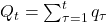 ), derived from the cointegrating relationship
  , establishes its own equilibrium with surface temperature (). Here,
  represents the total cumulative energy imbalance of the climate system—encompassing the oceans (the dominant reservoir), land, ice sheets, and the atmosphere. Following BCS (2020), ocean heat content serves as the empirical proxy for , since the oceans absorb the overwhelming majority of the accumulated imbalance; we acknowledge this is an approximation, as other reservoirs also contribute to the total energy stored.
This stored energy influences surface temperature through processes such as ocean heat uptake and release, spanning time periods far longer than regular weather cycles. Therefore, there may also be a long-run relationship between and . Define

Since and are both processes, if there exists a constant  such that
  is stationary, then by definition, and are cointegrated. In this case, a multicointegrated system is formed with two distinct equilibrium relationships: one between and , and another between their cumulative equilibrium error () and .
The importance of this second layer of cointegration is particularly evident in the climate context. For example, a permanent rise in radiative forcing due to industrial emissions could increase over decades and drive upward while also building up in the deep ocean. Over centuries, this stored oceanic heat is gradually transferred to the atmosphere, amplifying and creating a long-run feedback that multicointegration captures.
BCS (2020) applied the multicointegration framework within a parametric ECM using the MLE method of Johansen9. Such an approach is effective at capturing multiple long-run equilibria. However, it requires explicit parameterization of short-run dynamics. For example, it has to specify how the change in surface temperature this year is related to
  , the heat content flux two years earlier. Furthermore, it imposes Gaussianity on the VAR innovations, which is not plausible in our study, as we show in the empirical section.
Methodology: TAOLS Approach
The TAOLS method is a semiparametric estimator designed to estimate multicointegrating relationships with greater flexibility and reduced computational burden compared to the MLE method of Johansen9. We begin with the foundational cointegrating relationship:
(1) 
where is radiative forcing (in watts per square meter), is surface temperature (in degrees Celsius), is the cointegrating coefficient, and is the stationary error representing heat content flux. Cumulative sums are then defined as

Taking cumulative sums of Equation 1 and substituting  , we obtain the multicointegrating regression:

Here,  reflects the cointegration between cumulative forcing and cumulative temperature,
  represents the multicointegrating feedback from stored heat to current temperature, and represents unobserved random fluctuations.
Incorporating a constant and a linear time trend into the basic multicointegration model, we specify the empirical model as
(2) 
where the constant  and linear trend
  arise naturally from the multicointegration structure: including an intercept in the level equation , or equivalently in the lower-tier relation , generates a linear trend in the cumulative equation upon summation. The linear trend therefore allows for the possibility of a deterministic trend without imposing one—if no such trend is present in the data, the estimated coefficient
  will be indistinguishable from zero. Just as an intercept is routinely included in a regression to avoid misspecification, including the linear trend here is the appropriate default.
Following the framework of SPK (2025), we implement the TAOLS method through a three-stage process. First, we augment the model with the first difference in order to address endogeneity: long-run correlations between and would otherwise bias the estimates of and , since short-term fluctuations—such as a  El Niño spike—would contaminate the long-run estimates. The augmented model is
(3) 
Second, we project all variables onto a set of low-frequency basis functions. Specifically, we use the following sine functions:

Here ![r = t/T \in [0,1]](https://nhsjs.com/wp-content/ql-cache/quicklatex.com-31a3e5fbb0a2185025ea1141a55cc355_l3.png "Rendered by QuickLaTeX.com") is a normalized time index. In principle, any complete orthogonal basis can be used; the key requirement is that the first
is a normalized time index. In principle, any complete orthogonal basis can be used; the key requirement is that the first  basis functions have their energy concentrated at low frequencies, so that the transformation captures the long-run variation of the underlying integrated series. Sine functions, cosine functions, and Fourier (sine–cosine) pairs all satisfy this requirement. Following Phillips and Kheifets21, we adopt the above orthonormal sine basis. The corresponding transformed variables are
(4) 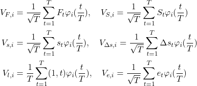
These transformed variables retain the low-frequency components of the time series while filtering out high-frequency variation. The parameter denotes the number of basis functions used in the transformation. Based on the transformed variables, we now have
(5) 
for  and
and  This is our transformed and augmented regression model.
Third, we apply OLS to the transformed regression model (Equation 13) to obtain estimates of ,  , , , and
  . Unlike Johansen’s MLE, which requires a fully specified ECM and assumes normality, TAOLS relies on the asymptotic properties of the transformed series, delivering estimators that are consistent and asymptotically mixed-normal under general conditions (e.g., weak dependence in ). A further advantage of TAOLS is that standard inference methods, such as the t-test, can be readily applied, making statistical inference straightforward. For details on the asymptotic theory, see SPK (2025).
Results
Data Sources
The empirical study uses data from BCS (2020), which was obtained from multiple sources and spans from 1850-2014, as detailed in Appendix A of BCS (2020). Radiative forcing is computed using an established formula for seven components: well-mixed greenhouse gases, solar irradiance, tropospheric sulfate aerosol, black carbon, organic carbon, ozone, and stratospheric aerosol. For example, the radiative forcing of carbon dioxide (CO), a critical greenhouse gas in climate research, is calculated using the logarithmic relationship:
(6) 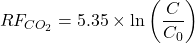
where  is the CO
 concentration in ppm, and
  is the pre-industrial level (1850), approximately 280 ppm. In the above,
  is an empirically derived coefficient from Myhre et al.22 that converts a change in CO concentration into a change in Earth’s radiative energy balance. We consider two versions of aggregate radiative forcing: full-efficacy radiative forcing (hereafter TotalRF) and partial-efficacy radiative forcing (hereafter MarvelRF), the latter adjusting the forcing from ozone, volcanic aerosols, and solar irradiance by a factor of 0.5.
Surface temperature data are sourced from Berkeley Earth23 and the Hadley Centre/Climatic Research Unit (HadCRUT)24. Temperatures, reported in Celsius, are expressed as anomalies relative to the January 1951–December 1980 average.
Figure 1 reproduces Figures 1 and 2 of BCS (2020), to provide a visual overview of the data. Panel (a) plots both radiative forcing series and panel (b) plots both surface temperature series. Radiative forcing and surface temperature display evident co-movement. However, the presence of large spikes induced by volcanic eruptions suggests that radiative forcing is unlikely to conform to a normal distribution. Consequently, applying a VAR system under the normality assumption, as implemented in BCS (2020), may yield unreliable estimates. The differences between the two versions of each series indicate some uncertainty in their measurement. If these differences are of a high-frequency nature, then TAOLS is particularly well-suited, as it does not rely on the high-frequency components of the underlying time series.
Stochastic Trend and Multicointegration Assumptions
The TAOLS framework requires that radiative forcing and surface temperature be each integrated of order one () and that the system is multicointegrated. These properties are supported by formal unit-root tests, physical reasoning, and the system-level rank tests reported by BCS (2020).
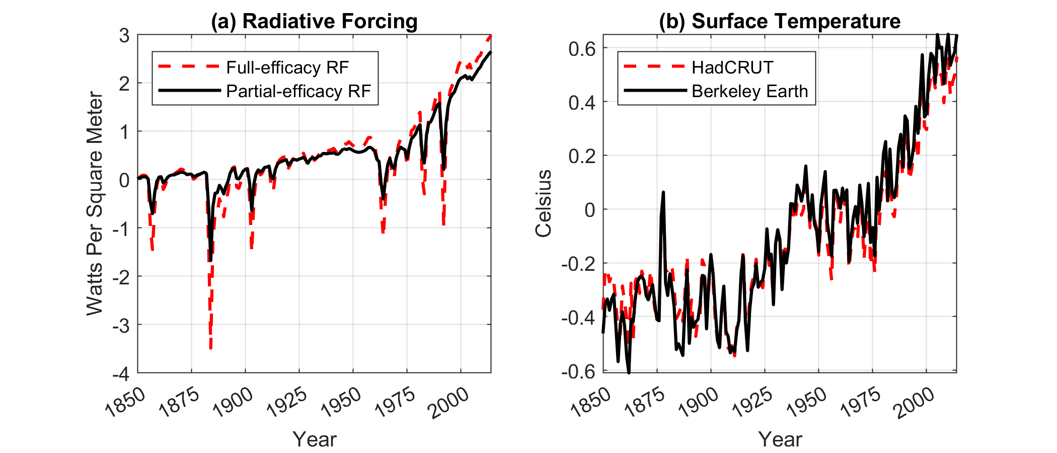
 ). Panel (b): Berkeley Earth and HadCRUT surface temperature anomalies (C, relative to 1951–1980).
Unit-root tests. We apply two complementary unit-root tests to all four series—TotalRF, MarvelRF, Berkeley Earth temperature, and HadCRUT temperature—over the full sample 1850–2014 ( ). The Augmented Dickey–Fuller (ADF) test25 has the null hypothesis of a unit root; failure to reject is evidence of behavior. The KPSS test26 has the null hypothesis of trend stationarity; rejection is evidence of a unit root. A pattern of ADF non-rejection combined with KPSS rejection thus constitutes strong evidence in favor of . For the ADF test, we include a constant (no deterministic trend) and select the lag length by BIC, up to a maximum of three lags. For the KPSS test, we use an automatic bandwidth selection procedure and test the null of trend stationarity. Table 1 reports the results.
| Series | ADF: Constant Stat (lag) p-val | KPSS: Trend Stat p-val |
| TotalRF | -1.653 (2) 0.449 | 0.921 ≤0.010 |
| MarvelRF | -0.1792 (2) 0.938 | 1.667 ≤0.010 |
| Berkeley | -0.073 (3) 0.950 | 1.481 ≤0.010 |
| HadCRUT | -0.098 (3) 0.947 | 1.635 ≤0.010 |
Notes: ADF H0: unit root; lag by BIC (max 3); 5% CV = -2.87. KPSS H0: trend stationary; 5% CV = 0.146, 1% CV = 0.216.
For all four series, the ADF statistic is well above the 5% critical value of  , so the null of a unit root is not rejected at any conventional significance level. Symmetrically, all four KPSS statistics far exceed the 1% critical value of
  , so the null of trend stationarity is strongly rejected. The two tests agree: every series is .
The characterization can also be based on physical reasoning and empirical evidence from the broader econometric literature. Radiative forcing is driven by the slow accumulation of greenhouse gas concentrations from persistent anthropogenic sources; surface temperature adjusts to forcing changes with a multi-decadal lag governed by ocean thermal inertia. As argued by BCS (2020) following Kaufmann et al.27, absent radiative forcing the climate system would be mean-reverting; it is because forcing itself follows a stochastic trend that temperature does likewise. Kaufmann et al.19 directly evaluate conflicting statistical claims about the integration order of surface temperature, including arguments in favor of trend-stationary representations, and conclude that the data cannot reject the unit-root characterization once the analysis is conducted carefully.
Moreover, BCS (2020) note, following Kejriwal et al.28, that a unit-root process is the limiting case of a trend-stationary process with a structural break every period: with enough breakpoints any random walk can be approximated by a piecewise linear trend-stationary process, making the two representations nearly observationally equivalent in samples of this length. BCS (2020) conduct Johansen  rank tests on the identical dataset and sample period, concluding that the two series are cointegrated and the system is multicointegrated. Since our analysis uses the same data and sample, these results carry over directly.
*Normality of innovations.* The Jarque–Bera (JB) test29 examines whether the skewness and excess kurtosis of a series are consistent with the Gaussian distribution. Because the level series are , we fit an AR(3) model,
![\[\Delta y_t = c + \rho_1\Delta y_{t-1} + \rho_2\Delta y_{t-2} + \rho_3\Delta y_{t-3} + \varepsilon_t,\]](https://nhsjs.com/wp-content/ql-cache/quicklatex.com-ce907f8079bfa5f8f8727a3c1e97d674_l3.png "Rendered by QuickLaTeX.com")
to each first-difference series by OLS and apply JB to the residuals. Removing autocorrelation structure before testing the distributional assumption provides a more stringent check of Gaussianity than applying JB directly to the first differences. The JB statistic ![\frac{T}{6}\bigl[S^{2}+\frac{(\kappa-3)^{2}}{4}\bigr]](https://nhsjs.com/wp-content/ql-cache/quicklatex.com-09bdd941f7aab7a786d9a3df354d94a2_l3.png "Rendered by QuickLaTeX.com") is asymptotically
is asymptotically  under the null, where
  and
and  denote sample skewness and kurtosis of the residuals (
 after three-lag alignment). Table 2 reports the results.
| Series | Skewness | Excess Kurtosis | JB Stat | p-value |
| ΔTotalRF | -1.019 | 8.131 | 471.3 | ≤0.001 |
| ΔMarvelRF | -0.893 | 7.870 | 436.9 | ≤0.001 |
| ΔBerkeley | 0.104 | -0.279 | 0.8 | ≥0.500 |
| ΔHadCRUT | 0.129 | -0.452 | 1.8 | 0.341 |
Notes: AR(3) model  , fitted by OLS. T = 161 residuals (1854-2014). H0: normality (). p-values bounded at 0.001/0.500 by MATLAB’s jbtest.
Both radiative forcing series reject normality decisively (JB  ,
,  ), driven by heavy-tailed outliers from major volcanic eruptions (e.g. Krakatoa in 1883, Pinatubo in 1991) that generate large year-on-year swings in forcing not captured by the linear AR(3) dynamics. By contrast, both temperature series are consistent with normality (
 ), reflecting the smoothing effect of ocean thermal inertia. This non-normality of radiative forcing innovations invalidates the Gaussian MLE used by BCS (2020) and provides the key motivation for TAOLS, which does not impose Gaussianity. Histograms and normal Q-Q plots are available upon request.
Multicointegration and ECS
Following BCS (2020), ECS is computed from the estimated cointegrating coefficient via
(7) 
where  is the radiative forcing from a doubling of CO concentrations (equation (RFCO2) with
  ). Although our empirical model uses aggregate radiative forcing, anthropogenic forcing over the instrumental record is dominated by long-lived greenhouse gases whose aggregate forcing is approximately proportional to CO forcing, so the CO-doubling benchmark remains the standard convention.
Our empirical analysis considers three data pairings from BCS (2020): Model I uses full-efficacy radiative forcing with Berkeley Earth surface temperature; Model II uses partial-efficacy radiative forcing with Berkeley Earth surface temperature; and Model III uses partial-efficacy radiative forcing with HadCRUT surface temperature. Strictly speaking, these are three data pairings rather than three separate models, but we use the same terminology for easy comparison.
Figures 2–4 display the TAOLS estimates of and the implied ECS for each data pairing. In Model I, ranges from  to
to  with a mean of
  , yielding ECS estimates in
 ![\left[1.82,2.16\right]^{\circ}](https://nhsjs.com/wp-content/ql-cache/quicklatex.com-ffb0af40f75130c50b94f669ed167ba7_l3.png "Rendered by QuickLaTeX.com") C with a mean of
C with a mean of  C. For Model II, lies in
 ![\left[1.488,1.750\right]](https://nhsjs.com/wp-content/ql-cache/quicklatex.com-d464406d7db3469e83ef21474e602254_l3.png "Rendered by QuickLaTeX.com") with a mean of
with a mean of  , corresponding to ECS in
 ![\left[2.12,2.49\right]^{\circ}](https://nhsjs.com/wp-content/ql-cache/quicklatex.com-ce8587f8d7f5fd9adb0068215050eb24_l3.png "Rendered by QuickLaTeX.com") C with a mean of
C with a mean of  C. In Model III, ranges from
  to
to  with a mean of
  , implying ECS in
 ![\left[1.81,2.05\right]^{\circ}](https://nhsjs.com/wp-content/ql-cache/quicklatex.com-4869bcce735016344b550197e610e6c9_l3.png "Rendered by QuickLaTeX.com") C with a mean of
C with a mean of  C.
C.
These results diverge from those of BCS (2020), who employed MLE within an ECM framework. Their MLE estimates of are ,  , and
, and  for Models I, II, and III respectively, implying ECS of C, C, and
  C. Across all three specifications, the TAOLS estimates of exceed the corresponding MLE values, yielding ECS estimates that range from C to C, all below the corresponding MLE benchmarks. Compared to BCS (2020), the standard errors of
  are generally smaller, producing narrower confidence intervals. In each specification, increases with but stabilizes around
  , beyond which additional basis functions have negligible effect on the estimates, a finding consistent with asymptotic efficiency arguments in SPK (2025).
A few comments on the choice of are in order. At the lower end, has to exceed the number of regressors in the TAOLS multicointegration regression (i.e., 5). Setting  leaves only
  residual degrees of freedom, the minimum we regard as adequate for reliable variance estimation; reducing to
  would exhaust all degrees of freedom (
 ), making the residual variance estimator undefined. The asymptotic standard error of each TAOLS coefficient is proportional to
  ; halving inflates the standard error by a factor of
  , which explains the wide confidence bands visible at
  . At the upper end, is bounded by the effective sample size after first-differencing (i.e.,
  ). Moreover, as
  , the TAOLS estimator converges to OLS, which suffers from an asymptotic bias that the sine transformation is designed to remove, so we stop short of at
  . While a data-driven choice of based on an asymptotic mean-squared-error criterion exists in principle, it cannot be estimated reliably at sample sizes of this magnitude. More importantly, quantitatively consistent estimates across the entire feasible range of —as we document here—provide stronger evidence of robustness than any single- result, which could reflect the particular frequency composition at that specific value of .
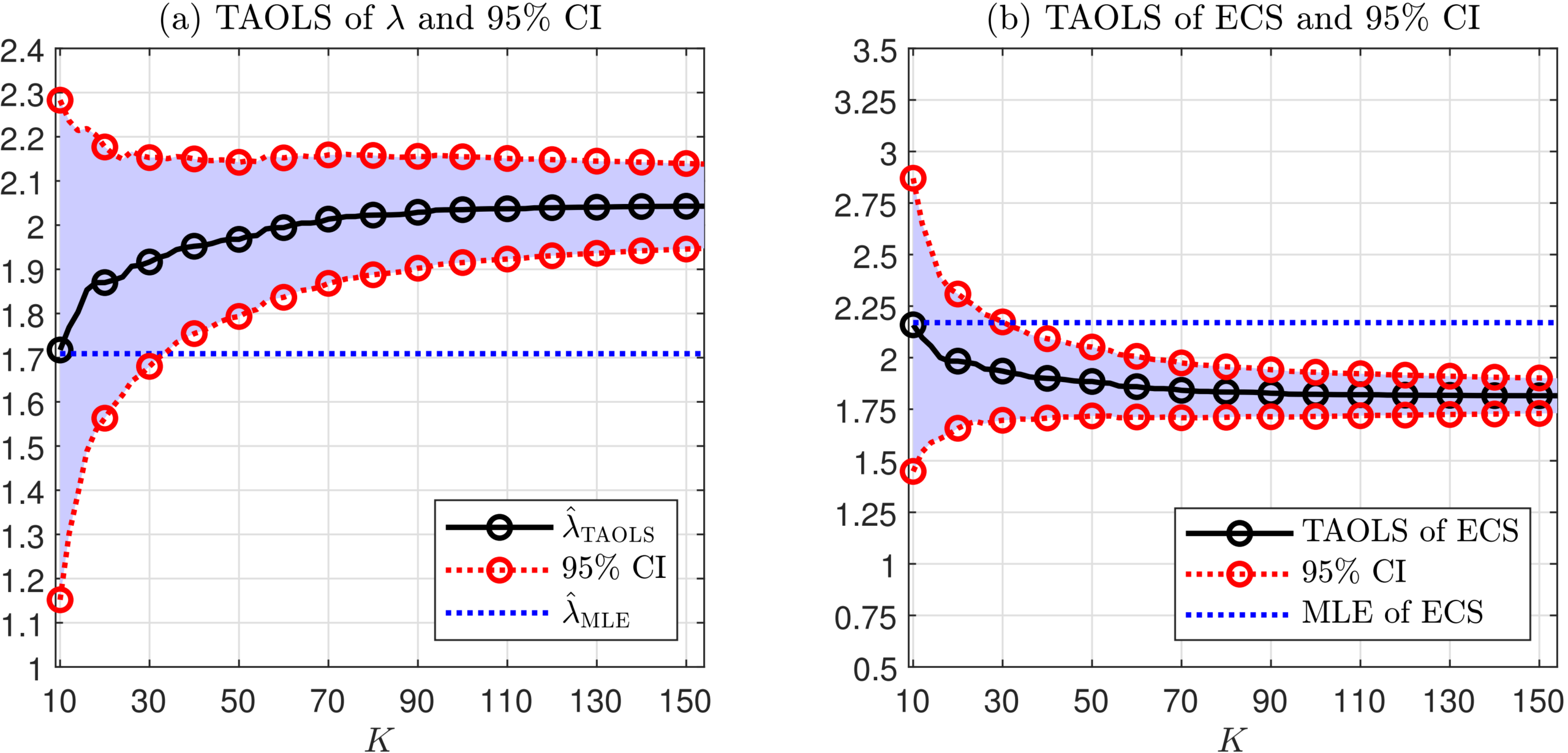 and the implied ECS in the presence of multicointegration for different values of using full-efficacy radiative forcing and surface temperature from Berkeley Earth (Model I). The shaded region represents the 95% confidence interval.
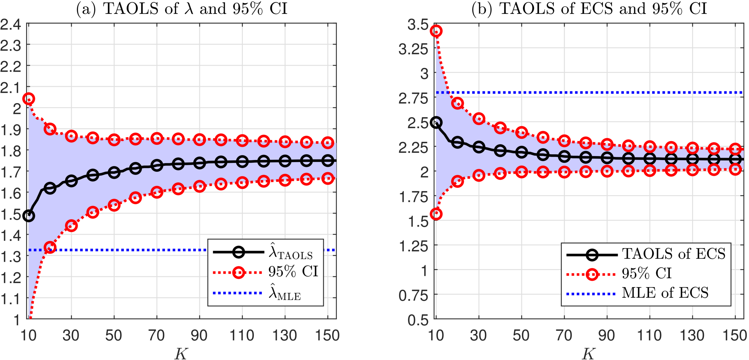 and the implied ECS in the presence of multicointegration for different values of using partial-efficacy radiative forcing and surface temperature from Berkeley Earth (Model II). The shaded region represents the 95% confidence interval.
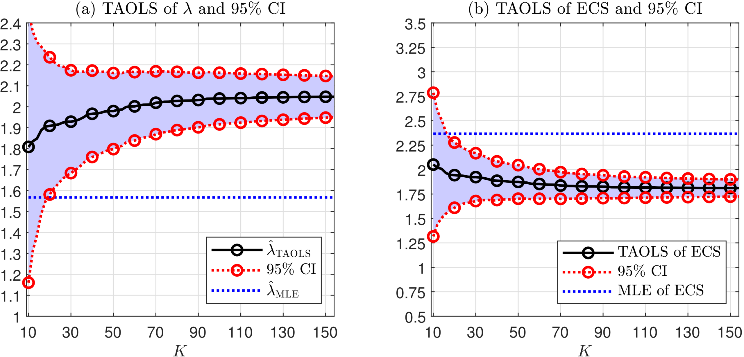 and the implied ECS in the presence of multicointegration for different values of using partial-efficacy radiative forcing and surface temperature from HadCRUT (Model III). The shaded region represents the 95% confidence interval.
Multicointegration and Heat Feedback
We now examine the estimate of in the model specified in (2). Note that measures the long-run relationship between the heat content of the system and surface temperature. At equilibrium, for a given value of , a rise in surface temperature by  C corresponds to an increase in the system’s heat content of approximately watt-years per square meter (W-yr/m
 ). For reference, according to (Oerlemans and van der Veen, 1984), increasing the atmospheric temperature by C requires approximately
  joules of energy, which translates to 0.31 W-yr/m. Thus, every 0.31 W-yr/m of additional heat absorbed by the atmosphere corresponds to W-yr/m of the total heat content of the entire system, including the atmosphere, oceans, and other components. This suggests that approximately
  percent of the total heat content contributes to warming the atmosphere.
For Model II, Figure 5 shows that the multicointegration parameter ranges from  to
to  across the values. To interpret this physically, consider
  : a
: a  increase in surface temperature corresponds to an additional
  W-yr/m of stored heat, predominantly in the oceans. This implies that
  percent of the total heat content contributes to atmospheric warming, with the remainder residing in oceanic or terrestrial reservoirs. By comparison, BCS (2020) reported values of 31 to 41, suggesting an air warming fraction of 1% or less.
Across all models, the estimated atmospheric share ranges from approximately 0.95% to 2.98%. This range closely matches the empirical estimate of roughly 1% for 1971–2018 reported in2. The agreement supports the conclusion that most excess heat is stored in the oceans rather than the atmosphere. Note that percent provides an underestimate of the fraction of ocean heat content directed toward surface warming, since the denominator reflects total system heat content rather than the ocean component alone; the difference is small given that the oceans dominate total system heat content.
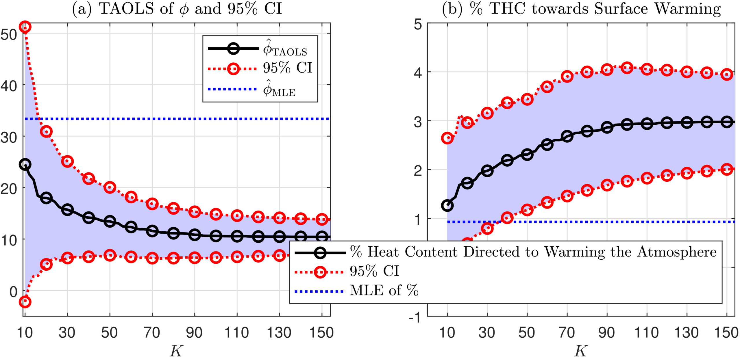 and the implied percentage of total heat content directed toward surface warming in the presence of multicointegration for different values of (Model II). The shaded region represents the 95% confidence interval.
To illustrate, suppose a sustained radiative forcing increase of  W,m over 10 years accumulates
  W-yr/m in . With , this heat storage corresponds to a surface temperature increase of approximately
  , illustrating the slow feedback from oceanic reservoirs to atmospheric conditions. This feedback mechanism illustrates why multicointegration is appropriate, as it captures dynamics beyond those described by cointegration alone.
For Models I and III, the estimates of are of comparable magnitude to those of Model II. In Model I (full-efficacy RF, Berkeley Earth), ranges from  to
to  W-yr/m, implying that approximately
  to
to  of the total heat content contributes to warming the atmosphere. In Model III (partial-efficacy RF, HadCRUT), ranges from
  to
to  W-yr/m, implying approximately
  to
to  . These ranges are broadly consistent with those of Model II and reinforce the conclusion that only a small fraction of accumulated heat content drives surface warming, with the remainder residing predominantly in oceanic reservoirs.
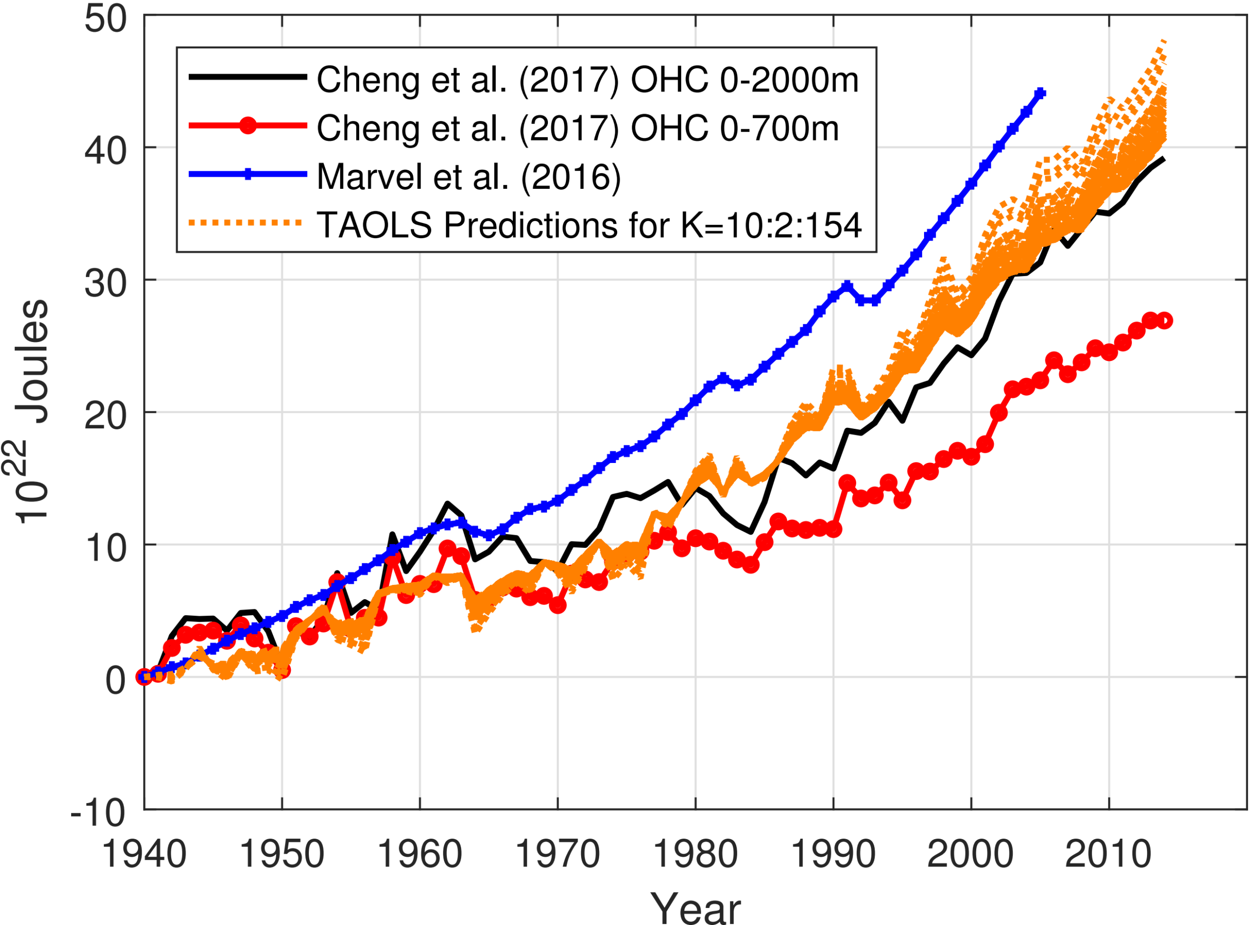
Following BCS (2020), Figure 6 plots the TAOLS-predicted system heat content against available ocean heat content observations for Model II (partial-efficacy radiative forcing with Berkeley Earth temperature). The model-implied cumulative Earth system heat content is converted to units of  Joules and scaled to the heat content of the top 2000,m of the ocean by multiplying by 0.81, following BCS (2020). The predicted sequence is compared with two observational benchmarks: observed ocean heat content in the top 0–2000,m and 0–700,m from Cheng et al.30 and the simulated series of Marvel et al.31, scaled to the top 2000,m by multiplying by 0.88. The TAOLS-predicted OHC series falls between the 0–700,m series of Cheng et al.30 and the series of Marvel et al.31, tracking the broad upward trend in ocean heat uptake since 1940. Results for Models I and III are quantitatively similar to those shown here.
Conclusions and Discussion
This paper applies the TAOLS estimator of SPK (2025) to the climate dataset of BCS (2020), providing the first application of TAOLS to climate data and a direct comparison of the TAOLS and MLE estimates of ECS. TAOLS is more robust than MLE because it does not impose Gaussianity on the model innovations and does not require precise specification of the short-run VAR dynamics—both assumptions that are difficult to maintain in climate time series that exhibit large non-Gaussian spikes from volcanic forcing.
Our ECS estimates from TAOLS, which range from  to
to  across all three data pairings, stand in contrast to higher estimates, such as those above
  from Bjordal et al. [14], which emphasize strong positive feedbacks (e.g., cloud dynamics). Our results also contrast with lower estimates, such as those below
  from Lewis and Curry [13], which some argue reflect the transient rather than equilibrium response. Compared to the MLE from BCS (2020), the TAOLS estimates are consistently lower across all three data pairings. We interpret this gap as evidence that the Gaussian VAR model underlying the MLE may be misspecified: when the innovations are non-Gaussian—as they are in climate data with large volcanic spikes—the MLE-based confidence intervals and point estimates can be unreliable, whereas TAOLS remains theoretically valid under weaker distributional assumptions.
The study has several limitations. The multicointegrating structure is maintained as an assumption, with supporting rank tests drawn directly from BCS (2020). All relationships are modeled as linear, abstracting from potentially nonlinear climate feedbacks14. The analysis uses global-mean data, setting aside regional heterogeneity, and the 165-year observational record is short relative to the multi-century equilibration time of the climate system BCS (2020). As a reduced-form econometric study, the estimates reflect the statistical properties of the data rather than the output of a mechanistic simulation.
This study suggests that the equilibrium temperature response to a doubling of CO is moderate and remains below
  , although this conclusion should be interpreted in light of the study’s limitations. If supported by future work, this result could have implications for climate policy. The analysis also shows that TAOLS can be applied successfully to climate time series. In this application, it produced credible estimates of climate sensitivity with narrower confidence intervals than MLE while avoiding Gaussian distributional assumptions and parametric VAR restrictions. These findings suggest that robust econometric methods may provide a useful alternative for empirical climate research.
Acknowledgments
The author expresses gratitude to Professor Jingjing Yang at the University of Nevada, Reno and Nie Jiawang at the University of California, San Diego for their guidance and encouragement throughout this project. The author also thanks an anonymous referee for detailed comments and suggestions.
References
- Karina von Schuckmann, Audrey Minière, Flora Gues, Francisco José Cuesta-Valero, Gottfried Kirchengast, Susheel Adusumilli, Fiamma Straneo, Michaël Ablain, Richard P. Allan, Paul M. Barker, et al. Heat stored in the Earth system 1960–2020: Where does the energy go? Earth System Science Data. Vol. 15, pg. 1675–1709, 2023, https://doi.org/10.5194/essd-15-1675-2023 [↩]
- IPCC. Climate Change 2021: The Physical Science Basis. Cambridge University Press, Cambridge, UK and New York, NY, USA, 2021. doi: 10.1017/9781009157896. URL https://www.ipcc.ch/report/ar6/wg1/. [↩] [↩] [↩] [↩]
- National Oceanic and Atmospheric Administration. Climate change: Atmospheric carbon dioxide. 2026. https://www.climate.gov/news-features/understanding-climate/climate-change-atmospheric-carbon-dioxide. Accessed: 2026-02-07. [↩]
- R. F. Engle, C. W. J. Granger. Cointegration and error correction: Representation, estimation, and testing. Econometrica. Vol. 55, pg. 251–276, 1987. [↩]
- C. W. J. Granger, T. Lee. Investigation of production, sales and inventory relationships using multicointegration and non-symmetric error correction models. Journal of Applied Econometrics. Vol. 4, pg. S145–S159, 1989. [↩]
- C. W. J. Granger, T. Lee. Multicointegration. In G. F. Rhodes, T. B. Fomby (eds.). Advances in Econometrics. Vol. 8, pg. 71–84. JAI Press. Greenwich, CT, 1990. [↩]
- Felix Pretis. Econometric modelling of climate systems: The equivalence of energy balance models and cointegrated vector autoregressions. Journal of Econometrics, 214(1):256–273, 2020. doi: 10.1016/j.jeconom.2019.05.013. [↩] [↩]
- Enrique Hillebrand, Felix Pretis, and Tommaso Proietti. Econometric models of climate change: Introduction by the guest editors. Journal of Econometrics, 214(1):1–5, 2020. doi: 10.1016/j.jeconom.2019.09.001. [↩]
- Søren Johansen. A representation of vector autoregressive processes integrated of order 2. Econometric Theory, 8:188–202, 1992. [↩] [↩] [↩]
- Stephan B. Bruns, Zsuzsanna Csereklyei, and David I. Stern. A multicointegration model of global climate change. Journal of Econometrics, 214(1):175–197, 2020. doi: 10.1016/j.jeconom.2019.05.010. [↩]
- Y. Sun, Peter C. B. Phillips, and Igor L. Kheifets. Estimation and inference in a possibly multicointegrated system with a fixed number of instruments. Economics Letters, 250:112297, 2025. doi: 10.1016/j.econlet.2025.112297. [↩]
- Gerard H. Roe and Marcia B. Baker. Why is climate sensitivity so unpredictable? Science, 318(5850):629–632, 2007. doi: 10.1126/science.1144735. URL https://www.science.org/doi/abs/10.1126/science.1144735. [↩]
- Lewis and Curry Nicholas Lewis and Judith A. Curry. The implications for climate sensitivity of AR5 forcing and heat uptake estimates. Climate Dynamics, 45(5):1009–1023, 2015. doi: 10.1007/s00382-014-2342-y. [↩] [↩]
- Jenny Bjordal, Trude Storelvmo, Kari Alterskjær, and Timo Carlsen. Equilibrium climate sensitivity above
 C plausible due to state-dependent cloud feedback. Nature Geoscience, 13(11):718–721, 2020. doi: 10.1038/s41561-020-00649-1. [↩] [↩] [↩]
 - Mikhail I. Budyko. The effect of solar radiation variations on the climate of the Earth. Tellus, 21(5):611–619, 1969. doi: 10.3402/tellusa.v21i5.10109. [↩]
- William D. Sellers. A global climatic model based on the energy balance of the earth-atmosphere system. Journal of Applied Meteorology, 8(3):392–400, 1969. doi: 10.1175/1520-0450(1969)008<0392:AGCMBO>2.0.CO;2. [↩]
- Jonathan M. Gregory, Ronald J. Stouffer, Sarah C. B. Raper, Peter A. Stott, and Nick A. Rayner. An observationally based estimate of the climate sensitivity. Journal of Climate, 15(22):3117–3121, 2002. doi: 10.1175/1520-0442(2002)015<3117:AOBEOT>2.0.CO;2. [↩]
- Robert K. Kaufmann and David I. Stern. Evidence for human influence on climate from hemispheric temperature relations. Nature, 388:39–44, 1997. doi: 10.1038/40332. [↩]
- Robert K. Kaufmann, Heikki Kauppi, Michael L. Mann, and James H. Stock. Does temperature contain a stochastic trend? Linking statistical results to physical mechanisms. Climatic Change, 118:729–743, 2013. doi: 10.1007/s10584-012-0683-2. [↩] [↩]
- Peter C. B. Phillips, Thomas Leirvik, and Trude Storelvmo. Econometric estimates of Earth’s transient climate sensitivity. Journal of Econometrics, 214(1):6–32, 2020. doi: 10.1016/j.jeconom.2019.05.001. [↩]
- Peter C. B. Phillips and Igor L. Kheifets. High-dimensional IV cointegration estimation and inference. Journal of Econometrics, 238(2):105622, 2024. doi: 10.1016/j.jeconom.2023.105622. URL https://www.sciencedirect.com/science/article/pii/S030440762300338X. [↩]
- Gunnar Myhre, Eleanor J. Highwood, Keith P. Shine, and Frode Stordal. New estimates of radiative forcing due to well mixed greenhouse gases. Geophysical Research Letters, 25(14):2715–2718, 1998. doi: 10.1029/98GL01908. [↩]
- Berkeley Earth. Berkeley Earth data: Global temperature and climate data. 2025. URL https://berkeleyearth.org/data/. Accessed: 2026-02-07 [↩]
- Met Office Hadley Centre and Climatic Research Unit. HadCRUT4 global surface temperature data, version 4.4.0.0. 2017. URL https://www.metoffice.gov.uk/hadobs/hadcrut4/data/4.4.0.0/download.html. Accessed: 2026. [↩]
- David A. Dickey and Wayne A. Fuller. Distribution of the estimators for autoregressive time series with a unit root. Journal of the American Statistical Association, 74(366):427–431, 1979. doi: 10.2307/2286348 [↩]
- Denis Kwiatkowski, Peter C. B. Phillips, Peter Schmidt, and Yongcheol Shin. Testing the null hypothesis of stationarity against the alternative of a unit root. Journal of Econometrics, 54(1–3):159–178, 1992. doi: 10.1016/0304-4076(92)90104-Y [↩]
- Robert K. Kaufmann, Heikki Kauppi, and James H. Stock. Does temperature contain a stochastic trend? Evaluating conflicting statistical results. Climatic Change, 101:395–405, 2010. doi: 10.1007/s10584-009-9711-2. [↩]
- Mohitosh Kejriwal and Carlos Lopez. Unit roots, level shifts, and trend breaks in per capita output: A robust evaluation. Econometric Reviews, 32(8):892–927, 2013. doi: 10.1080/07474938.2012.741063. [↩]
- Carlos M. Jarque and Anil K. Bera. Efficient tests for normality, homoscedasticity and serial independence of regression residuals. Economics Letters, 6(3):255–259, 1980. doi: 10.1016/0165-1765(80)90024-5. [↩]
- Lijing Cheng, Kevin E. Trenberth, John Fasullo, Tim Boyer, John Abraham, and Jiang Zhu. Improved estimates of ocean heat content from 1960 to 2015. Science Advances, 3(3):e1601545, 2017. doi: 10.1126/sciadv.1601545. [↩] [↩] [↩] [↩]
- Kate Marvel, Gavin A. Schmidt, Ron L. Miller, and Larissa S. Nazarenko. Implications for climate sensitivity from the response to individual forcings. Nature Climate Change, 6(4):386–389, 2016. doi: 10.1038/nclimate2888. [↩] [↩] [↩]