Abstract
As charging infrastructure, policy, and economic conditions change, electric vehicle (EV) adoption in the United States has been rapidly changing. However, the economy and infrastructure vary across states. This study utilizes past patterns to investigate and project future EV adoption throughout the US. The data are compiled manually from research and government sources. We then modeled the rates of EV adoption using a variety of different factors such as fuel and electricity prices, income, policies, and urbanization of different states. This research consists of a 2023 snapshot analysis, a spatial-temporal panel analysis of adoption from 2016 to 2023 over different states, and a growth prediction model for California using sigmoidal functions and Bass diffusion models. We found that higher income, greater gasoline prices, more incentives, higher vehicle use, and greater urban road ratios are positively associated with the adoption of EVs; on the other hand, higher electricity costs are negatively correlated with EV adoption. The results of spatial-temporal analysis show the effects of regional clustering. EV adoption has a tendency to spread from states that are closer together and have adopted EVs early. Using a logistic growth model, we forecast that California will reach ~50% EV adoption by 2035 before the rate of adoption flattens out. The logistic growth forecast is complemented by the Bass diffusion model, which shows that imitation dominates innovation for California data. Over the course of all of these findings, economic conditions and other factors are shown to be necessary in order for adequate future planning to continue EV adoption growth.
Keywords: electric vehicles, adoption, snapshot analysis, spatial-temporal panel analysis, growth prediction model
Introduction
Though the transition to electric vehicles (EVs) is often discussed as a technical and policy success, adoption is yet uneven across U.S. states. This raises a conceptual problem: given similar technological and national goals, why is adoption more concentrated in some places and lagging in others? This study treats EV adoption as a regional outcome shaped by differences in policy, infrastructure, prices, and demographics. This paper has three theoretical objectives. First, it tests which specific economic and policy factors, at the state level, are associated with adoption differences in 2023. Then, it evaluates whether adoption patterns from 2016 to 2023 are consistent with diffusion processes, which includes persistence over time, along with regional clustering across space. Third, the paper forecasts when California EV adoption will reach 50%.
Infrastructure access has been known as one main factor driving the adoption of EVs in many states. As of late 2023, the U.S. had a total of over 168,000 public EVSE charging ports, including more than 43,000 DC fast chargers1. However, access is unevenly distributed in many regions within the country. A study from the Pew Research Center has reported that 60% of urban residents live within two miles of a public charger; as a comparison, only 17% of rural residents have convenient access2. This urban-rural divide in access suggests possible barriers to usage among different groups of individuals.
The U.S. Department of Energy’s “eGallon” metric shows that, on average, fueling an EV remains less costly and less price-volatile than fueling a gasoline vehicle during current times3. Maintenance savings further strengthen the cost advantages of EVs. Despite this, overall transportation changes can show EV adoption as a transition in what consumers want. This shows how adoption of EVs is affected by more than just the cost of the vehicle. Factors such as changing infrastructure, policies, and the habits of consumers all affect the rate of EV adoption. We can also look at this from the perspective of social innovation. This is when growing familiarity and the growing use of a form of technology in people’s communities result in the growth of innovation. Through all of this, it is possible to help explain why adoption of EVs is different across states even though the economic conditions of these states may be similar. This research asks the following questions in order to further these objectives:
- Across U.S. states in the few years past (2023), what key factors are influencing EV adoption rates?
- From 2016 to 2023, how has EV adoption spread across different states? Can we predict EV adoption in the future using these patterns?
This study looks at three concepts: a 2023 snapshot analysis, a 2016-2023 spatial-temporal panel analysis, and a forecasting model for California. Through taking a variety of approaches, this study seeks to address both the current state of EV adoption and its projected trajectory for future implementation of policies and infrastructure.
The 2023 snapshot analysis provides an up-to-date picture of current U.S. EV conditions at the most recent point of complete data availability. Examining cross-sectional data allows us to evaluate how EV adoption is associated with potential factors. In addition to the six factors studied by Soltani-Sobh et al. (2017), we also include charging station density as a key measure of infrastructure availability4. Therefore, our cross-sectional snapshot analysis covers the following major economic, policy factors, and infrastructure variables: household income, fuel and electricity prices, financial incentives, and urban charging infrastructure density, miles per car, and urban road ratio. These indicators are selected based on established technology-adoption theory, which emphasizes the roles of affordability, relative cost advantages, and institutional support in shaping consumer adoption decisions.
The 2016-2023 panel analysis allows us to examine the diffusion of EV adoption over a period of time and across a variety of regions. By looking at multiple years, we can investigate patterns of growth as a result of time and regional clustering5. Finally, the California forecasting component projects future adoption in a state that is currently an EV leader in the U.S. California’s future trajectory can provide information about how an EV market may develop that may be applicable to other states as they continue with EV adoption.
Literature Review
Over the course of the past decade, new technology has been adopted at greater rates than ever before. For example, the number of EVs have been growing rapidly. A main part of this growth can be attributed to incentives for consumers such as environmental benefits and new policies. Furthermore, the response that consumers have to energy prices is asymmetric. In a study published by Xing et al. (2021), it is shown that EV sales are much more sensitive to gasoline prices than to electricity prices. What this means is that EV demand can be changed much more by cycles of oil prices than changes in electricity prices6.
Another reason for the changes in EV demand is due to growing availability and reliability of these vehicles. The number of non-home chargers (public + publicly accessible workplace) has reached approximately 204,000 on the national level by the end of the year 2024. Since 2019, this was considered approximately a 25% growth. This growth in the number of EV chargers provides families with a feeling of assurance for traveling long distances. Moreover, this also provides an incentive for purchase for households that currently do not have a garage where they can install EV chargers. Yet, it is also important to consider that a reduction in EV adoption can also result from the decreased reliability and uptimes of chargers in certain areas7.
Policies also encourage people to purchase EVs. For example, California’s Zero-Emission Vehicle mandate has encouraged manufacturers to invest in EV technologies and bring a wider range of electric vehicle models to the market8. Incentives such as HOV lane access can also significantly affect the number of registrations, especially for people who are living in areas that are much more busy9. Reductions in EV prices and faster ways to get more EVs on the road have also been incentivized by the Inflation Reduction Act passed on the federal level. By effectively reducing the upfront price of these vehicles, these programs are highly effective for increasing the number of EVs on the road.
However, there are still areas for further study in this growing amount of research. First, various studies use cross-sectional analysis or time series that cover the national level. Very few of these studies use spatial, temporal, and diffusion analysis together. Second, current research mostly focuses on sales rather than registration ratios in a region. By focusing on registration ratios, adoption in the long term can be better shown. Third, exponential and sigmoidal growth models are rarely compared using model selection criteria such as AIC. For these three reasons, this research looks at adoption and long-term growth of EVs through the use of diffusion models and analysis of regressions.
Methods
We compiled our own data by researching and compiling information from government and research institutes. This ensured that the data that were reputable and had accurate information that is relevant to our research question. We utilized datasets that met the following three criteria:
- Public availability and documentation
- Covers relevant years and information
- Data were complete
We then used Python to compile the data into a spreadsheet.
| Name of Source | Variable & Years Covered | Link to Source |
| U.S. Department of Energy Alternative Fuels Data Center | Electric Vehicle Count; 2016-2023 | 1 |
| Charging Station Count; 2023 | 10 | |
| Incentives Count; 2023 | 11 | |
| U.S. Energy Information Administration | Average Electricity Price; 2023 | 12 |
| Average Gas Price; 2023 | 13 | |
| U.S. Department of Transportation | Total Vehicle Count; 2015-2023 | 14,15 |
| Vehicle Miles Traveled, 2023 | 16 | |
| Urban Road Ratio, 2023 | 17 | |
| U.S. Census Bureau | Median Household Income; 2023 | 18,19 |
| Michigan State University Institute for Public Policy & Social Research | State-State Network Data: Policy Diffusion Tie (PDT), Border | 20 |
| Units | Mean | Median | Min | Max | |
| ElectricVehicles | vehicles | 70947.58 | 25833 | 959 | 1256646 |
| TotalVehicles | vehicles | 5685403.6 | 4536977 | 445240 | 31057329 |
| ElectricVehiclesRatio | proportion (0-1) | 0.008811 | 0.006396 | 0.000904 | 0.040462 |
| Income (median household) | 10000 USD | 76.9765 | 74.6315 | 54.203 | 99.858 |
| NumberofChargingStations | stations | 3720.58 | 1839.5 | 125 | 51097 |
| StateArea | sq. miles | 75933.52 | 57093.5 | 1545 | 665384 |
| ChargingStationDensity | stations/sq. mile | 0.100815 | 0.036778 | 0.000188 | 0.671025 |
| ElectricityCost | USD/kWh | 0.167002 | 0.1428 | 0.1098 | 0.4239 |
| GasCost | USD/gallon | 3.46362 | 3.374 | 3.086 | 4.907 |
| Incentives | count | 18.04 | 14.5 | 4 | 98 |
| TotalVehicleMilesTravelled | million miles | 64866.74 | 51823.5 | 5617 | 316612 |
| VehicleMilesTravelledPerCar | 10,000 miles per car | 1.1358 | 1.0984 | 0.5812 | 2.1826 |
| UrbanRoadRatio | proportion (0-1) | 0.318891 | 0.298434 | 0.033195 | 0.861813 |
Three new variables were derived from the compiled datasets: Electric Vehicles Ratio, Charging Station Density, and Vehicle Miles Traveled Per Car. Their definitions are shown in Table 3.
| Variable Created | Years Covered | Definition |
| Electric Vehicles Ratio | 2016-2023 | Divided number of electric vehicles by the number of total vehicles |
| Charging Station Density | 2023 | Divided number of charging stations by total state area |
| Vehicle Miles Traveled Per Car | 2023 | Divided total vehicle miles travelled by number of registered vehicles |
2023 Snapshot Analysis
Using data from 2023, we performed cross-sectional analysis to examine how factors affect EV adoption across the U.S. For this analysis, we define EV adoption rate as the proportion of EVs among all registered vehicles.
We worked on this analysis in different steps. In our first step, we tried to understand individual variables at the exploratory level. Next, we looked at relationships in pairs between adoption rate and various socioeconomic factors. Median household income, density of charging stations, price of gasoline, vehicle miles traveled per capita, urban road ratio, and whether incentives were present at the state level were examined. Then, we looked at and visualized the Pearson correlation coefficients.
Finally, we fit a multiple linear regression model to estimate the effects of each factor after adjusting other ones. In order to reduce redundancy in our model, we used Lasso regression and stepwise feature selection.
2016-2023 Spatial-Temporal Panel Analysis
This analysis examined both the spatial and temporal effects on adoption across states. To do so, we expanded our analysis to a 2016 to 2023 panel dataset. We utilized heatmaps and line plots to visualize EV adoption over the years for each state. We also decided to apply a log transformation to EV adoption rates because the log-transformed data shows a linear increasing trend over time.
Our spatial-temporal model is specified as follows. For state i at time t, the log-transformed adoption level is a function of (1) a state-specific effect, (2) a linear time trend, (3) a temporal lag (the previous adoption rate), and (4) two spatial lags: a lag for policy diffusion, and a lag for spillover effects from neighboring states that share a border.
![\[y_{(i,t)}=\alpha_i+\beta_1y_{(i,t-1)}+\beta_2t+\beta_3\sum_{j\neq i}w_{ij}^{Bor}y_{(j,t-1)}+\beta_4\sum_{j\neq i}w_{ij}^{PDT}y_{(j,t-1)}+\varepsilon_{(i,t)}\]](https://nhsjs.com/wp-content/ql-cache/quicklatex.com-ddab9a7fff1d6f22c2f58cf9ade66433_l3.png "Rendered by QuickLaTeX.com")
where
 : adoption level (after log-transformation) in state
  at time
 : state-specific fixed effect looking at unobserved heterogeneity across states
 : temporal effect, measuring the effect of a state’s own adoption in the previous year on its current adoption
 : linear time trend
 : spatial effect for states that share the same border, showing spillover effects from neighboring states’ past adoption,
  is proportional to the average adoption of neighboring states
 : policy diffusion tie effect, showing how adoption levels in states with policy diffusion ties to state ;
  is higher if policy network is more similar. The policy diffusion tie network information is part of the State-State Network Data, with information provided in Table 1.
 : error term
However, between the variables, there was high multicollinearity As a result, we also individually investigated how temporal effects, border sharing between states, policy diffusion ties, and trends in time affect adoption rates and compared the models.
Prediction for California
Among all the states, California stood out for our analysis. In California, there are very distinctive EV policies and infrastructure compared to other states. Furthermore, California was one of the earliest states to start the adoption of EVs. By modeling the adoption rate of EVs over time, we examined its pattern of EV adoption over time. We used three commonly used growth models to do this.
Exponential growth. California’s EV adoption rate was approximately linear after a log transformation. This shows how the exponential growth model may be suitable for showing EV adoption in the early stage, which is also the stage during which data are available. The following form shows the exponential growth function:
![\[f(t)=A\cdot e^{rt}\]](https://nhsjs.com/wp-content/ql-cache/quicklatex.com-e88180e2039971f1a78f72ed29628c14_l3.png "Rendered by QuickLaTeX.com")
where A is the initial adoption rate, r is the growth rate, and t is the time.
Sigmoidal growth. However, there are limitations to the exponential growth model. The main downside of the exponential growth model is that the model assumes EV adoption increases continuously at a constant rate. Furthermore, the exponential growth model assumes unlimited growth of EV adoption. However, in the real world, EV adoption rates are bounded between 0 and 1, so the exponential growth model is limited here. Therefore, sigmoidal models might be a better choice for this scenario. Through the use of sigmoidal models, we were able to predict what will happen many years later in terms of EV adoption. Sigmoidal functions all have the typical S-shaped trajectory of growth that starts slowly. Then, the curve steepens during the expansion phase and flattens out at the end to show that the market has been saturated. In this study, we utilized three commonly used sigmoidal functions:
- Logistic Growth Model:
where![\[f(t)=\frac{K}{1+e^{-r(t-t_0)}}\]](https://nhsjs.com/wp-content/ql-cache/quicklatex.com-4f475f9d682a83bc45b04dee4464a1a3_l3.png "Rendered by QuickLaTeX.com")
 is the carrying capacity,
  is the growth rate, and
  is the inflection point.
 - Gompertz Growth Model:
![\[f(t)=K\exp\left(-e^{-r(t-t_0)}\right)\]](https://nhsjs.com/wp-content/ql-cache/quicklatex.com-7bef0ece25c95379a946cd89eb616440_l3.png "Rendered by QuickLaTeX.com")
where, , are as above. Inflection occurs earlier than in the logistic model. - Richards Growth Model:
![\[f(t)=\frac{K}{\left(1+e^{-r(t-t_0)}\right)^{1/\nu}}\]](https://nhsjs.com/wp-content/ql-cache/quicklatex.com-b4e76f69d534f8295e7ffa33d098678d_l3.png "Rendered by QuickLaTeX.com")
where affects the asymmetry of the curve. This model generalizes the logistic model.
After this, we used the Akaike information criterion (AIC). By using AIC, we were able to compare the sigmoidal models that were described above to find out which model should be used for California’s EV adoption data. The reason that we did this is because AIC balances the complexity of the model along with the fit of the model. As a result of the Richards model having one more parameter than the other two models, this is better than relying purely on the model fit (such as likelihood).
Furthermore, we also utilized the Bass Diffusion Model on top of the growth functions. The Bass Diffusion Model uses behavioral factors that change adoption. Specifically, the model separates the adoption of EVs into two different mechanisms. These two mechanisms are the innovation effect and the imitation effect. The innovation effect shows how adoption of EVs early on was as a result of factors such as incentives of technology. The imitation effect shows how adoption is influenced by social contagion. Along with the S-shaped adoption curve, this model also shows us parameters with p for innovation and q for imitation. Moreover, the Bass model has also been used in other EV adoption studies21. By using the Bass model, we were able to find out what stage of EV adoption California is in.
Results
Cross-Sectional Determinants of EV Adoption (2023)
Figure 1 is a heatmap showing how EV adoption is most strongly correlated with incentives at the state level and income. Through this, we can see how higher income and better policies can allow for more EV adoption. We also found a moderately strong positive correlation in gasoline cost. Urban road ratio also has a moderate positive correlation. On the other hand, there is a weak correlation for charging station density with EV adoption. This suggests that infrastructure by itself may not increase adoption of EVs. Vehicle miles traveled per capita is negatively correlated with EV adoption.
We fit a simple linear regression for each feature in order to look at whether it is significantly correlated with EV adoption rate. All features, except charging station density, are significant at the 0.05 level.
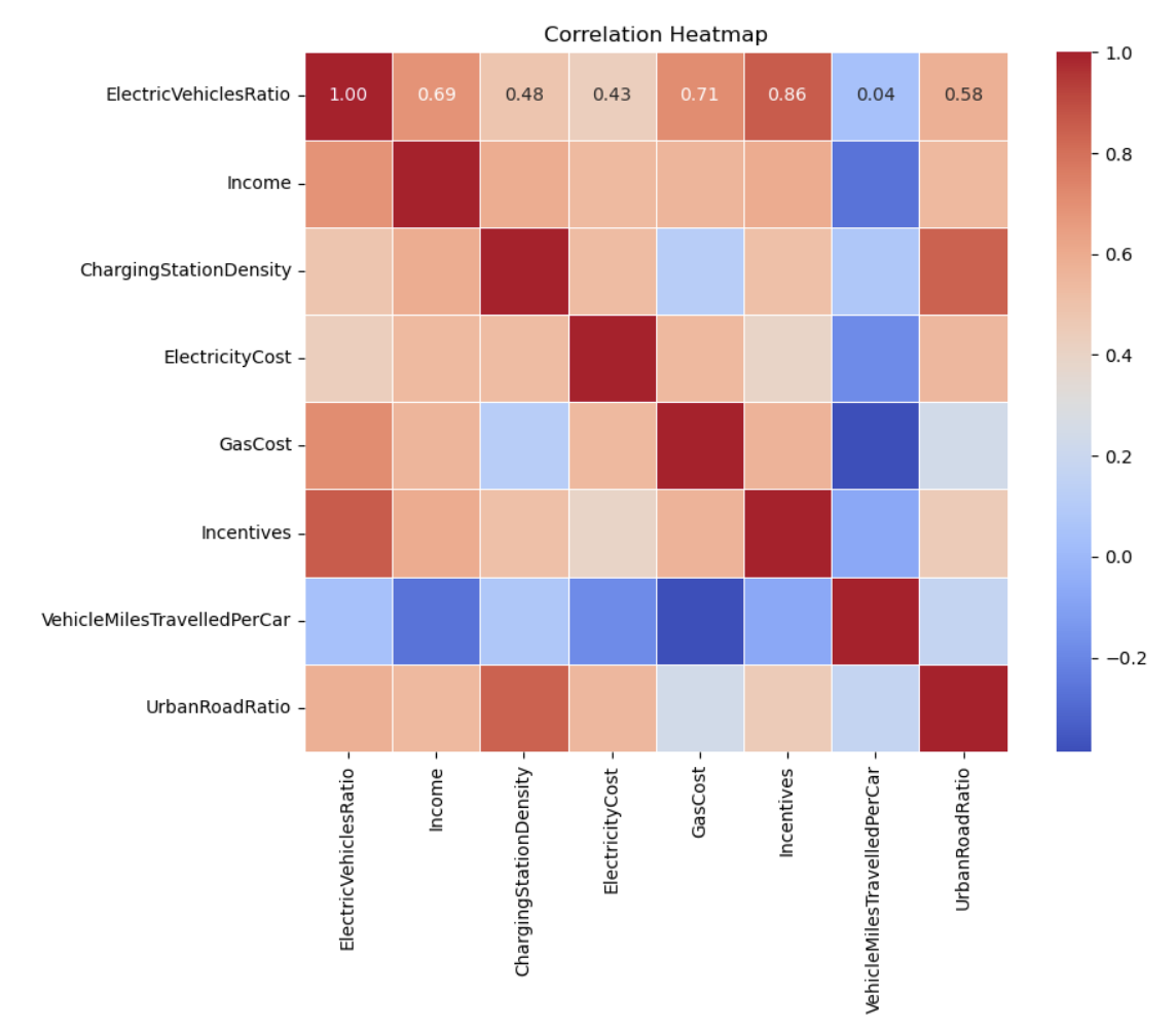
We conducted model selection by Lasso Regression, and forward and backwards selection in order to select features that help explain differing EV adoption across different states. Charging Station Density was dropped by both model selection methods We then analyzed the residual plot for the model and found no obvious outliers in our analysis. California originally seemed like an outlier individually but excluding it did not significantly affect the model that we were using.
| Estimated Coefficient | 95% CI | p-value | |
| Incentives | 0.02 | (0.017, 0.028) | 2.18x 10⁻¹⁰ |
| Gas Cost (dollar per gallon) | 1.02 | (0.76, 1.27) | 4.60x 10⁻¹⁰ |
| Miles per Car (10k miles) | 0.68 | (0.41, 0.96) | 1.04x 10⁻⁵ |
| Income (10k dollars) | 1.18 | (0.42, 1.94) | 3.14x 10⁻³ |
| Urban Road Ratio | 0.74 | (0.32, 1.16) | 9.51x 10⁻⁴ |
| Electricity Cost (dollar per kwh) | -2.12 | (-3.43, -0.80) | 2.29x 10⁻³ |
Table 4 shows the estimated effects of the six chosen variables: Gas Cost, Miles per Car, Income, Urban Road Ratio, Electricity Cost and Incentives. Incentives have a significant positive effect: each additional incentive is associated with a 0.02% increase in EV adoption (95% CI: 0.017% – 0.028%). This suggests that stronger policies at the state level are associated with higher EV adoption.
As expected, gas prices and electricity prices show opposite effects. Specifically, a one-dollar (per gallon) increase in gasoline price corresponds to about a 1.02% increase in EV adoption (95% CI: 0.76% – 1.27%), but a one-dollar per kWh increase in electricity cost corresponds to about a 2.12% decrease in EV adoption (95% CI: 0.80% – 3.43%). Together, these results show that the relative operating cost advantage of EVs compared with gasoline vehicles plays an important role in decisions of adoption in consumers.
The estimated effects show the importance of transportation behavior and built environment in EV adoption. Vehicle miles traveled per car and urban road ratio are both positively associated with EV adoption. A 100k-mile increase in annual miles traveled per vehicle is associated with about a 0.68% increase in EV adoption (95% CI: 0.41% – 0.96%), suggesting that higher driving intensity increases the potential cost savings from switching to EVs. Similarly, a higher urban road ratio is associated with greater EV adoption, indicating that more urbanized transportation increases EV adoption.
Lastly, median household income shows a positive association with EV adoption. An increase of $10,000 in median household income is associated with approximately a 1.18% increase in EV adoption (95% CI: 0.42% – 1.94%). Thus, higher-income states tend to have greater adoption. This is likely as a result of EVs involving a higher upfront cost despite lower operating expenses over time.
Overall, these results indicate that policy incentives, relative energy costs, driving intensity, socioeconomic conditions, and urban infrastructure all contribute to EV adoption. Among the factors examined, charging station density had a weaker effect with adoption. These results suggest that economic and policy variables explain a meaningful portion of variation across different states, while infrastructure at the state level may not fully show the same.
2016-2023 Spatial-Temporal Panel Analysis
For this part of the study, we first created a heatmap to visualize the change in EV adoption from 2016 to 2023 (Figure 2). We can see that adoption rates were fairly low nationwide in 2016. Only a few states such as California had early adoption that was noticeable. As time went on from 2017 to 2019, EV adoption expanded. The growth first occurred along the West Coast and a small region in the Northeast. By 2020 and 2021, EV adoption dramatically grew. In the heatmap, California and its neighbors have much darker shading, meaning higher EV adoption. By 2022 and 2023, the map shows that EV adoption has increased across the entire U.S. However, there were still major differences between regions with high adoption and regions with lower adoption. In 2023, California still had the highest adoption rate. On the other hand, states that are in the Mountain West or Southern region still have low levels of EV adoption. Examining the spatial and temporal trends, Figure 2 suggests that (1) EV adoption has become more nationwide and is no longer just for states that have started EV adoption early on, and (2) there are still drastic differences in EV adoption across different geographic areas.
This can also be understood through an idea known as energy justice. Energy justice is the concept that shows who benefits from transitioning to a different energy source and who is left behind. Higher-income states tend to have more policies encouraging EV adoption and more charging station access. This results in higher-income states receiving more of the benefits of transitioning from gasoline to electricity. However, on the other hand, lower-income and rural states tend to face challenges in this transition of energy. Furthermore, differences in social environment between states can also affect EV adoption. In some states, using an EV instead of a gasoline vehicle may be shown as a sign of environmental commitment in communities. In other states, however, environmental commitment may not be as socially rewarded. This results in slower EV adoption due to less incentives socially.
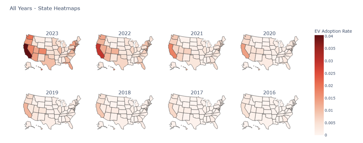
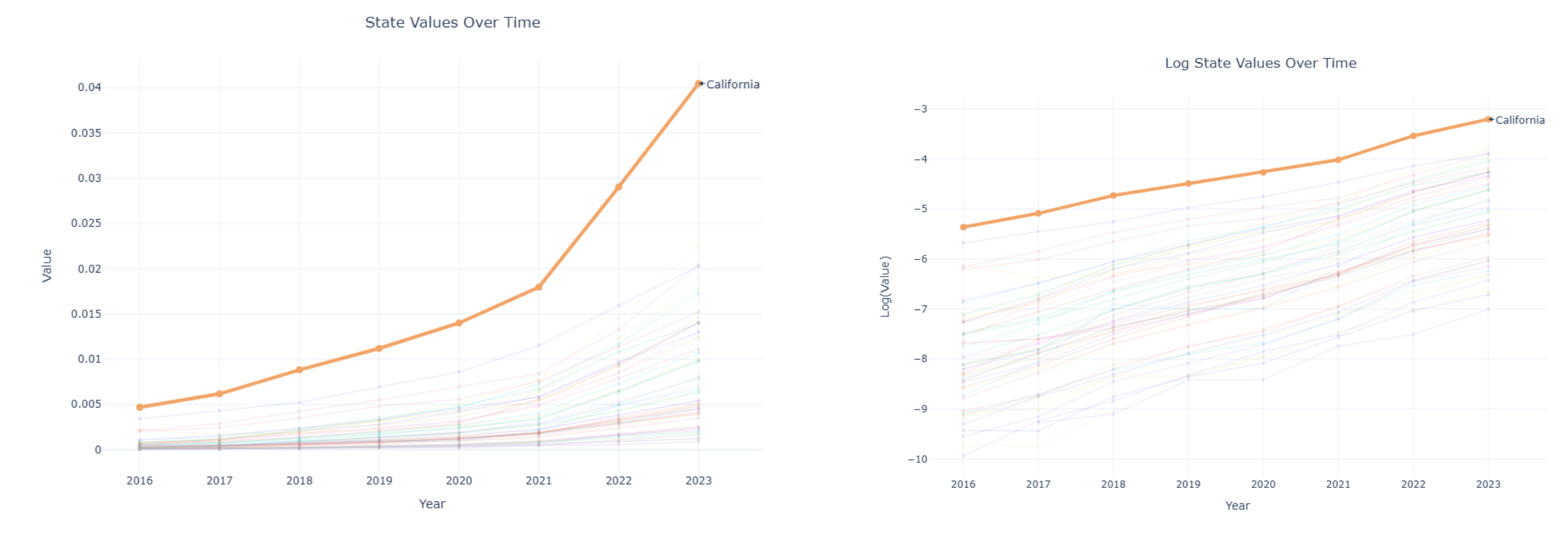
After this, we plotted lines over time to see how the values changed for each state. As shown in Figure 2, taking the log transformation for the lines After this, we plotted lines over time to see how the values changed for each state. As shown in Figure~2, taking the log transformation for the lines results in them appearing linear.
Initially, we wanted to include temporal lag, spatial lag, policy diffusion ties, and time in one model, as described in Methods. However, we found out that each of these four features is highly correlated. As a result, we decided to fit and compare the individual models:
| Model | Estimate (95% CL) | p-value | R2 | |
| EV_prev | EV_prev | 0.978 (0.956, 1.001) | <0.0001 | 0.959 |
| Time | Time | 0.414 (0.405, 0.423) | <0.0001 | 0.959 |
| EV_border | EV_border | 1.009 (0.985, 1.033) | <0.0001 | 0.958 |
| EV_PDT | EV_PDT | 1.038 (1.013, 1.063) | <0.0001 | 0.957 |
In Table 5, we can see that all four variables are significant at the 0.0001 level. Furthermore, each variable significantly affects EV adoption across states (R2 ≈ 0.96). After this, we also were able to find that these variables are highly correlated with each other. However, it would not be best to distinguish the contribution of each variable as a result of the strong collinearity. Nevertheless, we decided to fit a multiple regression model with all four of the variables. From this, we found that all variables are still significant. However, EV_border is only weakly significant (p=0.057) after adjusting for the other three factors. From the multiple regression, R2 was only increased very slightly (R2=0.978 and adjusted R2=0.974). This suggests that there may be an overlap in information shown by the variables.
We believe that the high collinearity is most likely as a result of the almost perfect linear growth trends after log transformation. This is shown in Figure 3. From the period of 2016 to 2023, EV adoption seemed to increase at similar rates nationwide. From this, we can infer that EV adoption in states can be predicted quite well no matter whether we use its own previous data or data from other states. As a result of this, we are not able to distinguish their effects from each other from the data alone. Spatial and policy variables only provide a slight improvement in the fit of the model. As a result of this, the results of the analysis should not be interpreted as causal effects of border effects. High collinearity does not allow us to separate time and effects from spatial variables.
Forecasting Adoption Trajectories: California Case Study
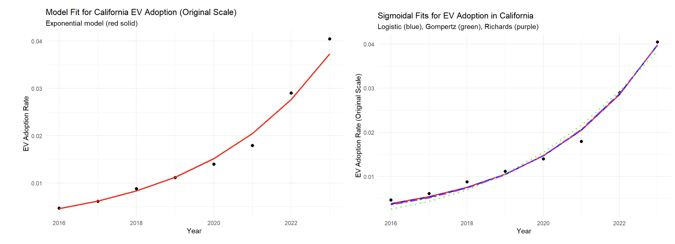
In this part of the study, we looked at California and the model’s predictions over time. We specifically wanted to focus on the year that EV adoption rate is predicted to be 50%. In Figure 4, the fitted growth curve using the exponential function and the three sigmoidal functions are shown.
In Figure 5, we can see that the exponential model on the left exceeds 100% at 2033, which is unrealistic in the real world.
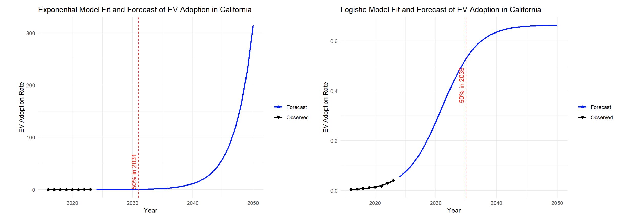
In Figure 5, the black dots near the bottom left of each graph show the EV adoption rates that were observed from 2016-2023. The blue curves are predicted values for the years 2024 to 2050. Unlike the exponential graph on the left showing unlimited growth, the logistic model (right) shows that adoption will eventually slow down and the graph flattens out. This occurs as a result of the market approaching saturation. This is what results in an S-shaped curve in the sigmoidal function. The vertical dashed red line shows the year that is predicted that California will reach approximately 50% EV adoption. In Figure 5, the exponential model predicts the year 2031 and the logistic model predicts the year 2035.
As a result of this, we decided to switch to sigmoidal models for our analysis. In our analysis, we preferred a smaller AIC value. Using AIC values, we decided that a logistic model is the best choice among the three sigmoidal models. In a logistic model, there is a carrying capacity that results in the flattening of the S-shaped curve. This carrying capacity shows how EV adoption rates will also flatten out as time goes on. By looking at the logistic growth model, half of California’s registered vehicles will be an EV by 2035.
We also compared EV adoption in other states similar to California. By doing so, we wanted to see how much time would pass before those states would appear like California in terms of EV adoption. To do this, we aligned the adoption rate of each state with that of California’s. Then, we compared how many years it would take for the 2016 value to reach that of California’s 2016 value.
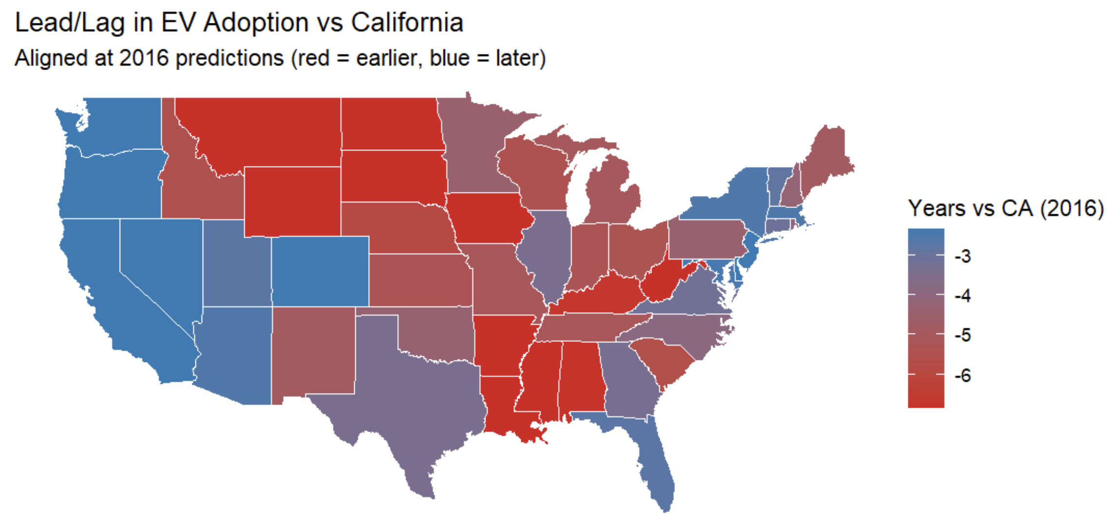
In Figure 6, the number of years each state lags behind California is represented in different colors, with red indicating larger lags while blue indicating smaller lags.
Finally, we ran a Bass diffusion model to evaluate the relative contributions of innovation and imitation to EV adoption. Although we were unable to get interpretable results with our 8 data points when we initially ran the Bass diffusion model, we were ultimately able to obtain data from California’s Energy website. This data ranged from 2010 to 202422.
| Variable Created | Estimate | Standard Error | t-value | Pr(>|t|) |
| p (innovation) | 0.0001357 | 0.0004456 | 0.304 | 0.766 |
| q (imitation) | 0.3219212 | 0.0337866 | 9.528 | 6.02e-07 |
| m | 1.0000000 | 3.5025890 | 0.286 | 0.780 |
From the Bass model, the estimation was a near-zero innovation coefficient. In California, this small value shows that adoption in California early on was affected by factors acting together rather than factors acting independently. The Bass model also produced a strong coefficient of imitation (q=0.3219, highly significant at p<0.0001). This shows the effect of contagion in EV adoption. In California, EV adoption is increasing because people in California see other people adopting EVs. When people see their neighbors, friends, and coworkers purchasing EVs, this incentivizes them to also purchase an EV for themselves. This trend can be similarly seen at a statewide level. When one state has policies and incentives affecting EV adoption, another state may be affected as well. From our findings, we found that in California, EV adoption rate will increase to 50% by 2035.
Discussion
Overview
This study focuses on a 2023 cross-sectional snapshot, a 2016-2023 spatial-temporal panel, and a California-focused forecast to explain why EV adoption differs across states and how EV adoption spreads over time. Together, our results were able to show patterns within states and across neighboring states. We were also able to consider how policies affect EV adoption.
This study relies on quantitative modeling. However, it is important to consider a variety of different factors when interpreting our results. Among such factors are sociology of innovation and the geographic distribution of economic policy. The concept of sociology of innovation suggests that the adoption of new technology is affected by social factors on top of changes in pricing of new technology. These social factors include the social networks that consumers are in as well as the norm of society in a specific region. The distribution of economic policy can show how states can be influenced to introduce new policy as a result of certain states being clustered together. This can affect how states introduce new incentives, resulting in changes in consumer behavior. By considering these concepts in our research, we were able to produce better regression and diffusion estimates. Not only did this allow our study to be more applicable for the broader context of society, considering these social factors also reduced the risk of interpreting economic factors as the only factors affecting EV adoption.
Factors Associated with EV Adoption
Economic capacity and policy support: In 2023, adoption was found to be most strongly tied to both state incentives and household incomes, as higher gasoline prices could encourage people to switch to EVs. When EVs are more affordable upfront, and fuel savings are more meaningful, adoption rates tend to rise.
Operating costs: Higher residential electricity prices are associated with lower EV adoption, since running costs of electric vehicles are more affected than those regarding gasoline vehicles.
Infrastructure and urban form: At the state level, charging-station density exhibits only a weak association and is no longer significant after accounting for incentives. This suggests that infrastructure availability might not operate as an independent driver of adoption at this scale. Instead, it might be closely intertwined with broader policy and institutional environments. Because charging-station density is correlated with income and incentives, infrastructure may function less as a direct causal factor and more as part of a state’s commitment to promoting EVs.
Travel intensity: Vehicle miles traveled per capita shows a negative correlation with adoption in our analysis. This suggests that more rural, long-distance driving makes EVs less favorable to some people.
Diffusion Across States
Adoption follows a diffusion pattern of starting on the West Coast and slowly moving eastward over time. This pattern suggests that adoption is influenced by more than prices alone. Regional clustering and spillover effects are consistent with the idea that EV adoption spreads through social and policy networks, as states learn from and respond to nearby early adopters. Log-transformed trends are close to linear, which shows how many states are still accelerating in terms of EV adoption. Persistence within states, neighbor effects, policy diffusion, and nationwide trends all impact EV adoption rates.
California as a Case Study
Model comparison favors a sigmoidal model. The logistic model projects that about 50% of registered vehicles in California will be electric around 2035, showing the acceleration of EV adoption while avoiding the over-prediction that comes with an exponential model. A Bass diffusion fit on a longer series shows a very small innovation effect and a large imitation effect. This shows how social contagion (adopting after peers) is very important to EV adoption rates.
Limitations
In our study, there are several limitations that must be considered. These limitations come from our data, modeling, and assumptions when forecasting.
Our study was conducted at the state level. As a result of this, we did not conduct analysis between the differences of individual states. Although our study researched differences between broader areas, we did not focus on the access of charging infrastructure at a specific local level. Past research has shown that EV adoption can be affected by different factors when smaller regions are considered. These smaller regions may be countries, ZIP codes, and neighborhood23. As a result of this, what changes EV adoption may vary within states. When we consider qualitative research, results show that the information available at a local level can be extremely important in changing EV adoption24,25,26.
When considering our forecasting results, it is important to consider these as projections rather than a precise prediction of EV adoption in the future. The reason for this is that diffusion models based on time trends may rely on certain assumptions that are oversimplified. When we analyzed the data using logistic and Bass models, the resulting graph was a smooth and continuous growth line. However, in the real world, there may be sudden changes in policy or consumer behavior. This results in EV adoption fluctuating rather than assuming the form of a smooth curve. As a result of not being able to model these factors, our model results are descriptive rather than causal.
Similarly, in our study, the spatial-temporal model only described patterns at a statistical level. The model that we used in this study cannot be used to prove causality for how EV adoption spreads. Lagged dependent variables and spatially lagged adoption numbers were used in our model. The result of this is that these two factors may be affected by each other or the results may be affected by external factors such as time trends.
The results of this study do not connect quantitative and qualitative factors together. Throughout our analysis, we used regression and diffusion models. It is vital to consider that these models are only for relationships statistically and the results of these models cannot be used to infer how consumers perceive the development and risk of new EV technology. From past research, we can see that decisions in terms of transportation are affected by a variety of different factors. Among such factors are social norms and the perception of convenience on top of economic incentives. Although mathematical patterns are informative, it is difficult to connect these results to personal experiences due to the lack of surveys and interviews. In order to understand how social factors influence EV adoption, it would be crucial for qualitative data to be collected as well.
For incentive policies, while our analysis focuses on the association between the number of incentives and EV adoption rates, it is also important to recognize that the adoption of these policies is driven by broader institutional and economic forces. Recent work shows that different types of policies exhibit heterogeneous effects and the quality and context of policies can matter as much as the number of policies27. Similarly, systematic reviews reported not all incentives are equal and EV adoption is driven by a complex interaction of institutional policy design and legal frameworks that go beyond mere monetary subsidies28. These findings suggest that interpreting correlations between incentive counts and adoption should account for underlying policy environments and economic interests that drive both policy choices and market outcomes.
Finally, the relatively short time (2016-2023) of the panel limits the feasibility of applying more advanced dynamic spatial panel estimators or instrumental-variable approaches. As a result, the estimated coefficients should be interpreted with caution. Future research using longer time series and advanced models would be needed to identify causal diffusion mechanisms more rigorously.
Policy Implications and Critical Synthesis
When people are incentivized financially, consumers are more likely to adopt EVs. However, this also depends on a state’s ability to pass new legislation and which consumers can realistically use EVs for everyday transport. Although implementing new incentives can reduce the cost upfront, these new incentives may also result in a new problem. When new incentives are introduced, they may increase the gap between those who are already able to adopt EVs and those who are not in a position to adopt yet.
It is also important to recognize that electricity prices affect the appeal of owning an EV for consumers. Although states can implement higher pricing during peak times or encourage consumers to use home chargers, it is vital to recognize that not all households can change the way they use their EVs or install chargers at home.
When considering how charging access can be expanded, especially in rural areas, it is crucial for urban planners to consider which regions receive this type of investment first. The chargers that are installed should be reliable, easy to access for consumers, and easy to maintain for the companies who installed these chargers.
From our analysis, we found that EV adoption appears to be clustered in regions. This suggests that if neighboring states coordinate with each other, EV adoption can increase at a greater rate. When states coordinate with each other, it is also important to recognize that different states may have different development goals and commitments.
International Context
This research focused only on the United States. However, the diffusion of EVs can also be affected at an international level. For example, in Norway, the government introduced large purchase incentives and charging access policies that differ from the U.S. but allowed Norway to reach a high proportion of EVs. This case can also be seen in China. Through industrial policy and supporting the large-scale manufacture of EVs, China was able to drastically expand EV adoption. These international examples show that EV adoption depends on the context of each individual nation and EV findings of one nation should not be used to generalize to other countries.
Summary
Not only are there economic considerations for EV adoption, but there are also various social factors. EV adoption tends to be drastically different between rural and urban areas as well as between wealthy areas and regions struggling with poverty. When states have higher income levels and better infrastructure, EV adoption tends to be higher. On the other hand, areas with less charging infrastructure and that are more rural tend to have greater barriers for EV adoption. Some of these obstacles that rural areas face include a lack of support from local governments and a long travel distance to charging stations.
Many individuals believe that EV adoption will increase through a reduction of consumer cost. Although this is true to some extent, the introduction of new EV public policy is what will truly increase EV adoption. Well-designed public policy can affect technological progress by decreasing the inequality of access between less-developed areas and wealthier regions, allowing access to new and exciting technology for everyone.
Acknowledgements
The authors thank the UCI ICS Summer Academy 2024, where they first met and discovered a shared interest in studying energy efficiency. MJ also appreciates the opportunity to learn data science through UCI COSMOS. They are grateful to their mentors, Professor Tingting Nian UCI, for her very helpful comments such as the suggestion of Bass diffusion models.
References
- Alternative Fuels Data Center: Vehicle Registration Counts by State. (2023). Energy.gov. https://afdc.energy.gov/vehicle-registration?year=2023. [↩] [↩]
- Bestvater, S., Shah, S. (2024). Electric Vehicle Charging Stations Across the US. Pew Research Center. https://www.pewresearch.org/data-labs/2024/05/23/electric-vehicle-charging-infrastructure-in-the-u-s/. [↩]
- US Department of Energy. (2013, 6). eGallon. https://www.energy.gov/sites/prod/files/2013/06/f1/eGallon-methodology-final.pdf. [↩]
- Soltani-Sobh, A., Heaslip, K., Stevanovic, A., Bosworth, R., & Radivojevic, D. (2017). Analysis of the Electric Vehicles Adoption over the United States. Transportation Research Procedia, 22. https://www.sciencedirect.com/science/article/pii/S235214651730162X. [↩]
- Soltani-Sobh, A., Heaslip, K., Stevanovic, A., Bosworth, R., & Radivojevic, D. (2017). Analysis of the Electric Vehicles Adoption over the United States. https://www.sciencedirect.com/science/article/pii/S235214651730162X. [↩]
- Xing, J., Leard, B., & Li, S. (2021). What does an electric vehicle replace? Journal of Environmental Economics and Management, 107(102432). https://doi.org/10.1016/j.jeem.2021.102432. [↩]
- Powell, B., & Johnson, C. (2025). Impact of Electric Vehicle Charging Station Reliability, Resilience, and Location on Electric Vehicle Adoption. Publications. https://docs.nrel.gov/docs/fy24osti/89896.pdf. [↩]
- Mcconnell, V., Leard, B., & Kardos, F. (2019). California’s Evolving Zero Emission Vehicle Program: Pulling New Technology into the Market. rff.org. https://media.rff.org/documents/RFF_WP_Californias_Evolving_Zero_Emission_Vehicle_Program.pdf. [↩]
- Sheldon, T. L., & DeShazo, J. R. (2017). How does the presence of HOV lanes affect plug-in electric vehicle adoption in California? A generalized propensity score approach. Journal of Environmental Economics and Management, 85(146-170). https://doi.org/10.1016/j.jeem.2017.05.002. [↩]
- Energy.gov. (2025). Historical Station Counts. Energy.gov. https://afdc.energy.gov/files/docs/historical-station-counts.xlsx?year=2023. [↩]
- Alternative Fuels Data Center: Maps and Data – Electric Vehicle Laws and Incentives by State. (n.d.). Afdc.energy.gov. https://afdc.energy.gov/data/10373. [↩]
- EIA. (n.d.). Average Electricity Price. Eia.gov. https://www.eia.gov/electricity/annual/xls/epa_02_10.xlsx. [↩]
- EIA. (2023). Average Gas Price. Eia.gov. https://www.eia.gov/state/seds/sep_sum/html/xls/pr_ex_mg.xlsx. [↩]
- Federal Highway Administration. (2023). Table MV-1 – Highway Statistics 2023 – Policy. Federal Highway Administration. https://www.fhwa.dot.gov/policyinformation/statistics/2023/mv1.cfm. [↩]
- Transportation.gov. (2023). Motor Vehicle Registrations, 2000 – 2023 (MV-1). Transportation.gov. https://data.transportation.gov/Roadways-and-Bridges/Motor-Vehicle-Registrations-2000-2023-MV-1-/4dra-vxq7/about_data. [↩]
- Federal Highway Administration. (2023). Table VM-2 – Highway Statistics 2023 – Policy. Federal Highway Administration. https://www.fhwa.dot.gov/policyinformation/statistics/2023/vm2.cfm. [↩]
- Federal Highway Administration. (2023). Table HM-20 – Highway Statistics 2023 – Policy. https://www.fhwa.dot.gov/policyinformation/statistics/2023/hm20.cfm. [↩]
- Engel, K., & Posey, K. G. (2024). Household Income in States and Metropolitan Areas: 2023. Census.gov. https://www2.census.gov/library/publications/2024/demo/acsbr-023.pdf. [↩]
- United States Census Bureau. (2023). Income in the Past 12 Months. <a href="https://data.census.gov/table/ACSST1Y2023.S1901?q=S1901&g=010XX00US
 0400000. [↩]
 - Institute of Public Policy and Social Research. (2020). State Networks. https://ippsr.msu.edu/public-policy/state-networks. [↩]
- Lee, J., Hardman, S., & Tal, G. (n.d.). Who is buying electric vehicles in California? Characterising early adopter heterogeneity and forecasting market diffusion. Energy Research & Social Science, 55. https://www.sciencedirect.com/science/article/abs/pii/S2214629618312258. [↩]
- New ZEV Sales in California. (n.d.). California Energy Commission. http://www.energy.ca.gov/data-reports/energy-almanac/zero-emission-vehicle-and-infrastructure-statistics-collection/new-zev. [↩]
- Cervini, G., Jung, J., & Gkritza, K. (2024). Temperature and electric vehicle adoption: A ZIP code-level analysis in the US. Transportation Research Part D: Transport and Environment, 136(104435). https://www.sciencedirect.com/science/article/abs/pii/S1361920924003924 [↩]
- Krishna, G. (2021). Understanding and identifying barriers to electric vehicle adoption through thematic analysis. Transportation Research Interdisciplinary Perspectives, 10(100364). https://www.sciencedirect.com/science/article/pii/S2590198221000713. [↩]
- Tomkins, S., Yin, S., Vaishnav, P. et al. Quantifying real and perceived barriers to EV adoption in rural Michigan. Sci Rep 16, 2742 (2026). https://doi.org/10.1038/s41598-025-32478-w. [↩]
- Palinkas, L., Liff, M., Campos, A., Martinez, A., Eckel, S., Chen, F., Johnston, J., Franco, W., & Garcia, E. (2025). A co-created, community-informed model for electric vehicle adoption in disadvantaged communities. Transportation Research Part D: Transport and Environment, 146(104853). https://www.sciencedirect.com/science/article/pii/S1361920925002639. [↩]
- Mekky, M., & Collins, A. (2024). The Impact of state policies on electric vehicle adoption -A panel data analysis. Renewable and Sustainable Energy Reviews, 191(114014). [↩]
- Anastasiadou, K., & Gavanas, N. (2022). State-of-the-Art Review of the Key Factors Affecting Electric Vehicle Adoption by Consumers. MDPI. https://www.mdpi.com/1996-1073/15/24/9409. [↩]