Developing and Evaluating AI Models for Classifying Bone Tumors Using X-ray Imaging

Abstract

As the core algorithms and underlying infrastructure for artificial intelligence (AI) have become mature, it is critical to integrate state-of-the-art AI capabilities across various science and engineering disciplines to solve societal problems, particularly those involving labor-intensive, repetitive tasks with learnable outcomes. One emerging area for AI integration is radiology. X-ray imaging is a primary tool used in classifying a bone tumor, but the volume and complexity of images can make human diagnosis inefficient and inaccurate. Even experienced musculoskeletal radiologists achieve only about 83-84% accuracy when classifying primary bone tumors as benign or malignant on radiographs, making it an ideal use case for AI assistance. In this paper, we obtained a set of X-ray images of primary bone tumors released in 2025, and developed three AI models to classify tumors as benign or malignant. In particular, this work developed a multi-layered perceptron (MLP), a convolutional neural network (CNN), and ConvNext, an enhanced version of CNN developed by Meta. We conducted comprehensive performance evaluations on Google Colab and studied the impact of various hyperparameters across all three models. Our results show that AI models can achieve up to 89% accuracy, demonstrating strong potential to support radiologists in a diagnostic task known to suffer from substantial inter- and intra-observer variability, and to accelerate and improve bone tumor classification.

Keywords: AI, image classification

Introduction

As the core algorithms and underlying infrastructure for artificial intelligence (AI) have become increasingly mature, it is critical to integrate state-of-the-art AI capabilities across various science and engineering disciplines to solve societal problems, particularly those involving labor-intensive, repetitive tasks with learnable outcomes. This is particularly true for medicine, where the diagnosis of certain diseases is heavily dependent on local features (e.g., the shape and size of a tumor), which AI models can be trained with. By identifying these features in the data and using AI models to make inferences, medical facilities can now use high-performance computers to rapidly pre-screen patients and recommend potential diagnoses to physicians, thereby greatly improving the efficiency and quality of healthcare. Particularly in radiology, X-ray imaging is a primary tool to detect and stage many types of cancer, including bone, breast, and lung cancer. However, the volume and complexity of X-ray images in a large medical facility can make human diagnosis inefficient and error-prone, especially during a pandemic such as COVID-19. Although AI models have inherent uncertainties and may not fully replace radiologists in the near future, AI recommendations can greatly accelerate diagnosis and prioritize treatment for the most critical patients.

There has been extensive research interest in applying AI models to interpret X-ray images with mixed clinical results to date. AI-assisted interpretation has shown diagnostic performance comparable to a radiology resident in emergency department chest radiographs^1,2. However, bone cancer has far more varieties and higher complexity due to a wide range of locations where the bone tumor can occur, from the upper limb to the lower limb, and the pelvis. Bone cancer is usually suspected through symptoms, such as pain and swelling, and primarily diagnosed through imaging, such as X-ray or MRI scans. Bone cancer diagnosis through imaging by radiologists is not always accurate. X-ray is a very labor-intensive process, and interpretation of bone tumor radiographs is subject to substantial variability even amongst trained specialists. A 2025 study found poor agreement amongst orthopedic residents and oncologists when classifying radiolucent bone lesions using standard radiographic grading systems³. As such, there has been strong interest from the radiology community in leveraging new AI capabilities to assist physicians, not only to accelerate the diagnostic process but also to increase diagnostic accuracy.

Contributions. The primary objective of this study is to evaluate and compare the effectiveness of three deep learning architectures: multi-layer perceptron (MLP), convolutional neural network (CNN), and ConvNext, for classifying primary bone tumors as benign or malignant using the recently released BTXRD X-ray dataset. The contributions of this paper are as follows:

1. This paper uses state-of-the-art neural networks to automatically classify bone tumors from a large volume of tumor images. In particular, we developed a simple MLP, various CNN architectures, and the recently developed ConvNext, which has been shown to outperform vision transformer architectures on medical image classification tasks⁴.
2. We conduct comprehensive hyperparameter tuning and performance evaluations on Google Colab to understand the effectiveness of the AI models. The results show that the AI models can achieve up to 89% accuracy, demonstrating the potential of using AI to assist physicians by automatically classifying tumors as benign or malignant.
3. We evaluate model performance using a comprehensive set of metrics beyond overall accuracy, including per-class precision, recall, F1-score, sensitivity, specificity, ROC-AUC, and AUPRC, together with repeated stratified k-fold cross-validation and 95% confidence intervals, to account for the class imbalance in the dataset.
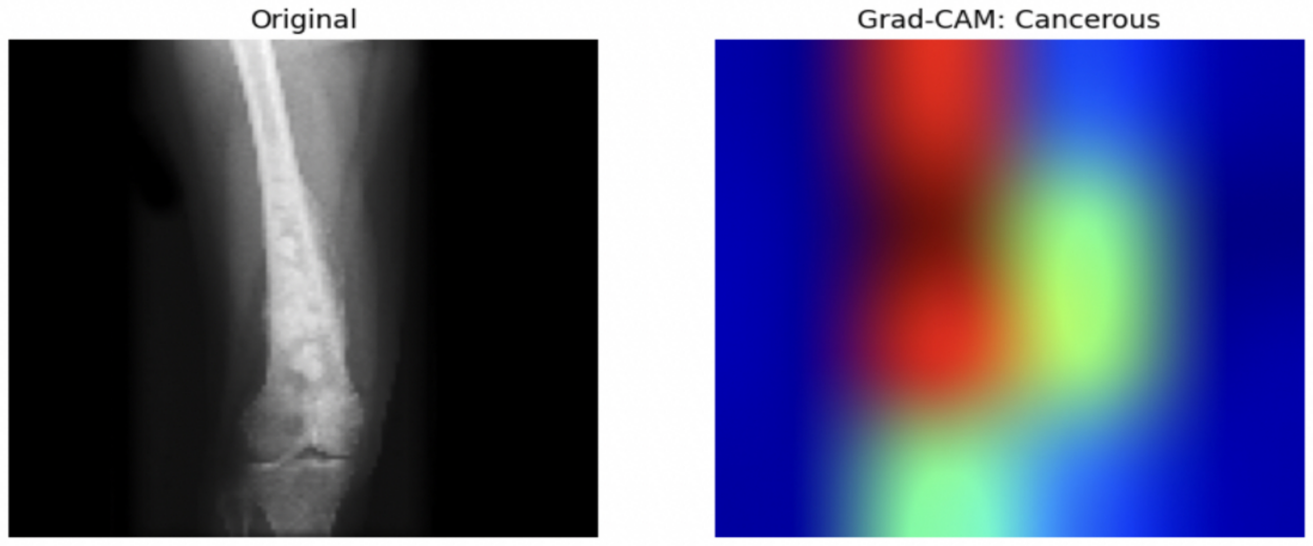
4. We provide explainability analysis using Grad-CAM to verify that model predictions are driven by tumor-relevant image regions, rather than irrelevant artifacts, which supports the clinical plausibility of the models.

Literature Review

Beyond the work previously discussed, a growing amount of research has applied deep learning specifically to primary bone tumor imaging. Several groups have targeted radiograph-based classification: Long et al. developed a model that improved classification of primary bone tumors even when X-ray, CT, and MRI inputs are incomplete for a given patient⁵. Von Schacky et al. proposed a multitask network that segments and classifies primary bone tumors on plain radiographs⁶. Dalai et al. built an automated bone cancer detection pipeline trained on X-ray images⁷. Wang et al. trained deep learning models to classify primary bone tumors and distinguish them from bone infections, which is a related but unique diagnostic task⁸. Other works have extended beyond radiographs to histopathology and CT: Borji et al. proposed a hybrid deep learning model for evaluating osteosarcoma histopathology images⁹. Walid et al. developed a voting classifier that combines deep learning models for osteosarcoma classification¹⁰. Li et al. introduced EENet, a CNN-based framework for bone tumor pathological diagnosis¹¹. Sampath et al. compared several CNN architectures for early bone cancer diagnosis using CT images¹². Aziz et al. combined deep feature extraction with a multilayer perceptron classifier for osteosarcoma classification, an architectural pairing related to the MLP and CNN models we will evaluate¹³. More recently, Song et al. developed an interpretable machine learning and radiomics model to distinguish osteosarcoma from chondrosarcoma in a multicenter retrospective study¹⁴, while Anisuzzaman et al. presented an earlier deep learning approach for detecting osteosarcoma from histological images¹⁵. A 2025 narrative review surveys this broader work on AI in primary malignant bone tumor imaging¹⁶. Taken together, this literature shows that bone tumor classification has been approached through a range of methods (CNN, MLP, hybrid models), but remains constrained by small, single-institution, and imbalanced datasets, which motivates the present study’s use of a larger, recently released radiograph dataset^17,18.

Parallel work in other cancer types offers useful architectural context for the models compared in this paper. For breast cancer, Setiawan et al. applied the classification¹⁹, and Yuan et al. compared CNN and transformer-based architectures on breast cancer histopathology images⁴. Lu et al. combined multimodal imaging with deep learning radiomics to distinguish benign from malignant breast tumors²⁰, a binary classification task structurally similar to the benign/malignant classification task we will be addressing for bone tumors. A 2025 study combined CNNs with generative adversarial networks to classify ovarian tumors as benign, malignant, or borderline²¹, and Liu et al. applied a multilayer perceptron-based model to classify histological subtypes of lung adenocarcinoma²². A multibranch CNN combined with an MLP-Mixer module has also been proposed for disease diagnosis more broadly²³. Collectively, these studies indicate that CNN, MLP, and hybrid CNN-MLP designs are actively used across cancer imaging tasks, with no single architecture established as objectively superior. Our paper aims to address this directly for bone tumors by benchmarking MLP, CNN, and ConvNext under matched conditions.

A separate line of research has evaluated how AI performs when benchmarked against or alongside radiologists in practice. Guo et al. compared radiologist performance on chest X-ray diagnosis with and without AI assistance¹¹. Kumar et al. conducted a service evaluation of an AI diagnostic tool’s ability to recognize normal chest radiographs in a live clinical workflow²⁴. A 2025 systematic review synthesized agnostic accuracy data from multiple AI-assisted cancer radiology studies²⁵. These studies display how the growing use of AI-assisted screening is being actively evaluated as a complement rather than a replacement to radiologist judgment.

Because the BTXRD dataset used in this study is imbalanced (1,525 benign to 342 malignant tumor cases), the literature on class imbalance in medical image classification is directly relevant to the limitations of this study. Walsh and Tardy compared several techniques for addressing class imbalance in deep learning-based breast cancer classification²⁶. Yoshitsugu et al. proposed a random upsampling method for numerical features to improve classification sensitivity on imbalanced medical datasets²⁷. A 2024 study examined how class imbalance affects deep learning performance across medical imaging tasks more generally²⁸. A related line of work proposed a one-class classification approach for handling imbalanced medical image data²⁹. This body of work suggests that resampling, cost-sensitive training, or one-class classification are promising directions for future extensions of this study, given the underrepresentation of malignant cases in the current dataset.

Finally, methodological parallels can be drawn from existing COVID-19 imaging literature, which similarly involved rapidly assembled, often imbalanced datasets. Enhanced CNN and transfer learning approaches have been applied to COVID-19 detection from chest X-rays³⁰, and a large empirical study benchmarked deep transfer learning methods for COVID-19 classification across both CT and X-ray methods³¹. These studies illustrate how pretrained, transfer learning-based architectures, the same strategy used for the ConvNext model in this paper, have been applied under similarly constrained data conditions in other disease domains. Table 1 provides a comprehensive comparison between this study and previous works.

Study	Dataset/Sample Size	Imaging Modality	Framework/Model	Validation Strategy	Performance Metrics
Song et al. 20245	1,305 patients (internal n=1043; external n=262), 2 centers, 2010-2022	X-Ray, CT, MRI (incomplete multimodal)	PBTC- TransNet (transformer based multimodal fusion)	Internal test set + independent external test set (retrospective, 2-center)	Micro-avg AUC 0.847 (internal), 0.782 (external); accuracy 84.3% (X-ray only subgroup, internal)
Von Schacky 20216	934 patients internal (667 benign, 267 malignant); 111 patients external test	Radiographs (X-ray)	Multi Task deep learning CNN (joint detection + segmentation + classification)	654 train/ 140 val/ 140 internal test + 111-patient external test	Accuracy 80.2% sensitivity 62.9% specificity 88.2%
Dalai  et al. 20257	Not specified in accessible abstract (healthy vs cancerous X-rays)	X-ray	SqueezeNet feature extraction + Golden Search + improved cuckoo + LSTM	Train/test split (proportions not specified in accessible abstract)	Accuracy 95.52% (training), 94.79% (testing)
Wang  et al. 20258	Internal: 1044 train/ 354 test/ 171 val; External: 423 patients; multicenter	Radiographs + clinical features	Ensemble of EfficientNet-B3, EfficientNet-B4, ViT, Swin Transformer + ML fusion layer	Two step 5 fold cross validation (imaging models + clinical feature fusion) + independent external test set	AUC 0.948 (internal), 0.963 (external); accuracy 88.1% (external); comparable to radiologist (83.6%)
Borji  et al. 20259	TCIA public osteosarcoma histopathology dataset	Histopathology	Hybrid CNN + Vision Transformer (ViT)	Train/test split on public dataset (first 4-class classification reported on dataset)	Accuracy 99.08% precision 99.1%, recall 99.28%, F1-score 99.23%
Walid  et al. 202310.	Public osteosarcoma H&E histology dataset , rebalanced via augmentation	Histopathology	Custom CNN + heterogeneous ensemble voting classifier	70%/30% train test split with data augmentation for class balance	Kappa score 93.09% (proposed CNN alone); 96.5% (voting ensemble, best)
Li et al. 202411	N/A	N/A	EENet (CNN-based)	N/A	N/A
Sampath  et al. 202412	Small CT dataset of 3 bone cancer subtypes	Histopathology	Multiple pre trained CNNs compared	N/A	Accuracy 95.52% (training), 94.79% (testing)
Aziz  et al. 202313	Public osteosarcoma WSI (whole-slide image) dataset (TCIA)	Histopathology	Hybrid: pretrained CNN deep feature extraction + MLP classifier	Train/test split; feature selection ,method chosen by execution time and accuracy	Accuracy 95.2% (3-class: non tumor/necrosis/viable), 99.4% (binary classification)
Song et al. 202414	76 patients, 2 centers (Guizhou Medical University), Jan 2018-Jan 2024	CT (radiomics: 788 shape/texture/first order features)	Random Forest, Extra Trees, AdaBoost, Gradient Boosting, LDA, XGBoost	Multicenter retrospective train/validation with SHAP based interpretability	Best model (Random Forest): AUC around 1.00; Extra Trees AUC 0.98; AdaBoost AUC 0.93
Anisuzzaman  et al. 202115	Public TCIA osteosarcoma histology dataset (UT Southwestern/ UT Dallas)	Histopathology	Transfer learning with pre trained CNNs (VGG19 best, among others compared)	Binary and multiclass (non-tumor/necrotic/viable) classification tasks, train/ test split	Best model (VGG19): 96% accuracy (binary and multiclass classification)
Our study	BTXRD:1525 benign, 342 malignant (80/20 train test split)	X-ray	MLP, CNN, and ConvNext	Single held out 80/20 train test split	Accuracy up to 89% (ConvNext, best performing model)

In what follows, we further discuss related computational models, including Vision Transformer (ViT), Swin Transformer, EfficientNetV2, ConvNext-V2, ConvNext-V2, Hybrid CNN-Transformer Models.

ViT applies pure self-attention over image patches and achieves strong results, but it lacks the inductive biases, e.g. locality and translation equivariance, that CNNs have built in. This means ViT typically needs very large pretraining datasets or heavy augmentation/regularization to match CNN performance on smaller datasets. ConvNext was explicitly designed to test whether an advanced CNN – incorporating design choices from transformers (larger kernels, layer norm, GeLU, inverted bottlenecks, fewer activation functions) – could match ViT/Swin performance without abandoning convolutional inductive bias.

Swin introduced hierarchical feature maps and shifted window attention to make transformers more CNN-like (multiscale, locality via windows), specifically to support dense prediction tasks (detection, segmentation). ConvNext was designed as a direct counterpoint: it shows that a hierarchical convolutional network can match Swin’s accuracy on classification, detection, and segmentation benchmarks, without the computational overhead of windowed attention or the complexity of shifted window masking.

EfficientNetV2 optimizes for training speed and parameter efficiency via neural architecture search combined with progressive learning. However, it can be less flexible to adapt/modify for downstream tasks and is optimized against a specific search objective, which doesn’t always transfer cleanly across hardware or tasks. ConvNext is designed via a systematic ablation from ResNet, making its design choices more interpretable and its scaling behavior more transferable across tasks.

ConvNext-V2 is the direct successor to the original architecture, integrating a fully convolutional masked autoencoder pretraining framework and a Global Response Normalization layer to address feature collapse in the network’s channels. It shows consistent gains over ConvNext-V1 across model sizes, particularly when self-supervised pretraining is available. Hybrid architectures aim to combine early stage convolutional inductive bias with later stage global attention, often achieving strong accuracy and efficiency trade offs. Their drawback is architectural complexity. Mixing operation types complicates deployment, quantization, and hardware optimization, and often requires more careful hyperparameter tuning to balance the two paradigms. ConvNext’s contribution shows that hybridization may be unnecessary, since most of the performance gains attributed to attention mechanisms can be recovered with pure convolutions if modernized appropriately.

Methods

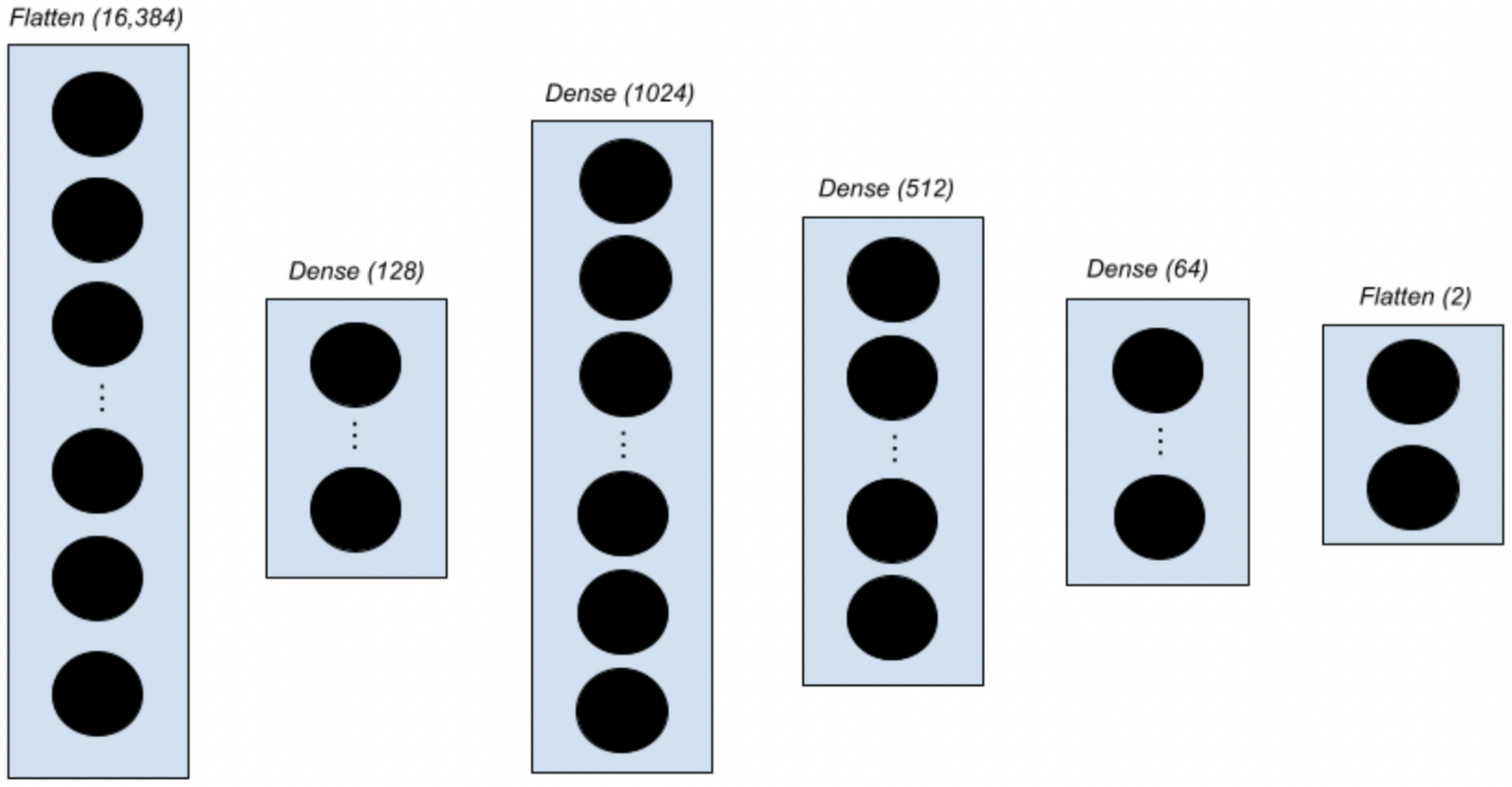
Multi-layer Perception. First, we develop an MLP network with four hidden layers (Figure 1). MLP is a feedforward neural network consisting of fully connected layers, in which each neuron is connected to all neurons in the next layer. In our default MLP model, we have four hidden layers, each with 128, 1024, 512, and 64 neurons, respectively. For each layer, we use ReLU as the activation function. In particular, the input layer takes a 128×128 image and flattens it into 1D, and the final layer has two neurons with softmax activation.

CNN. Given the wide adoption of CNNs in image classification, this work also develops a CNN model for bone tumor classification. In general, a CNN model consists of the following four layers: a convolutional layer, an activation layer, a pooling layer, and a fully connected layer for classification. They are described next:

• The convolutional layer utilizes trainable filters (also known as kernels) to produce feature maps that detect specific patterns in an image, such as edges, shapes, and colors. Deep convolutional layers learn more sophisticated patterns, such as combinations of features (e.g., corners).
• The activation layer further allows the model to learn nonlinear relationships between patterns.
• The pooling layer downscales the dimensions of feature maps by summarizing local regions, thereby reducing computational cost and parameter count.
• The fully-connected layer serves as the model classifier by connecting all neurons in a given layer to every neuron from the previous layer, and captures complex and global relationships among features.

By default, our CNN is configured to have 11 layers. The first layer has 32 trainable 3×3 filters, and the activation function is ReLU. This layer is followed by a max pooling layer with a window size of 2×2. Other downstream convolutional layers have 64, 128, and 256 filters, respectively. These layers are then followed by two dense layers with 128 and 2 neurons, respectively, with the latter using softmax as the activation function.

ConvNext. ConvNext is a modern convolutional neural network architecture built on the traditional CNN model, incorporating design improvements from state-of-the-art deep learning models. Similar to traditional CNNs, ConvNext retains the core components of convolutional layers for feature extraction, activation functions to capture non-linear patterns, and fully connected layers for classification. However, ConvNext has several enhancements that improve inference performance and efficiency. First, it uses larger filters to capture more complex patterns within images. Second, ConvNext uses layer normalization, instead of the batch normalization often used in CNNs, to improve training stability, especially with varying batch sizes. Batch normalization works by normalizing the input across the entire batch, meaning the output depends on other samples in the batch, which can often lead to instability when batch sizes are small or inconsistent. To address this problem, ConvNext adopts layer normalization, which normalizes features within a single sample, making it independent of batch size and more stable during training. Third, ConvNext adopts depthwise separable convolutions, which improve computational efficiency by reducing the number of parameters while still capturing features. Finally, ConvNext simplifies the overall network architecture by using strided convolutions instead of traditional pooling layers for downsampling. Strided convolutions downsample feature maps using learnable filters that preserve important spatial patterns, whereas traditional pooling layers use static downsampling, which can lead to loss of information.

List 1 shows the Python code that uses ConvNext for image classification. By default, the ConvNext model used in the paper is configured using a pretrained ConvNextBase architecture with ImageNet weights, with the classification layer removed. By default, all layers of the base model are unfrozen to allow for model fine-tuning. The backbone is followed by a global average pooling layer to reduce feature maps, then a dense layer with 128 neurons using ReLU activation. A dropout layer with a rate of 0.5 is applied for regularization. The final layer is a dense layer with 2 neurons using soft activation for classification. A reduced learning rate of 0.00001 is used during fine-tuning and is implemented with the Adam optimizer, to allow the pretrained weights to be updated gradually without disrupting previously learned features.

Listing 1: Python code for using ConvNextBase model for classification

# 1. Load the ConvNeXtBase model

base_model = ConvNeXtBase(include_top=False, weights=’imagenet’, input_shape=(image_size[0], image_size[1], 3))

# 2. Unfreeze all layers of the base model for fine-tuning

base_model.trainable = True

# Create a new sequential model

model = tf.keras.Sequential([

   base_model,

   GlobalAveragePooling2D(),

   Dense(128, activation=’relu’),

   Dropout(0.5),

   Dense(num_classes, activation=’softmax’)])

Experimental Setup

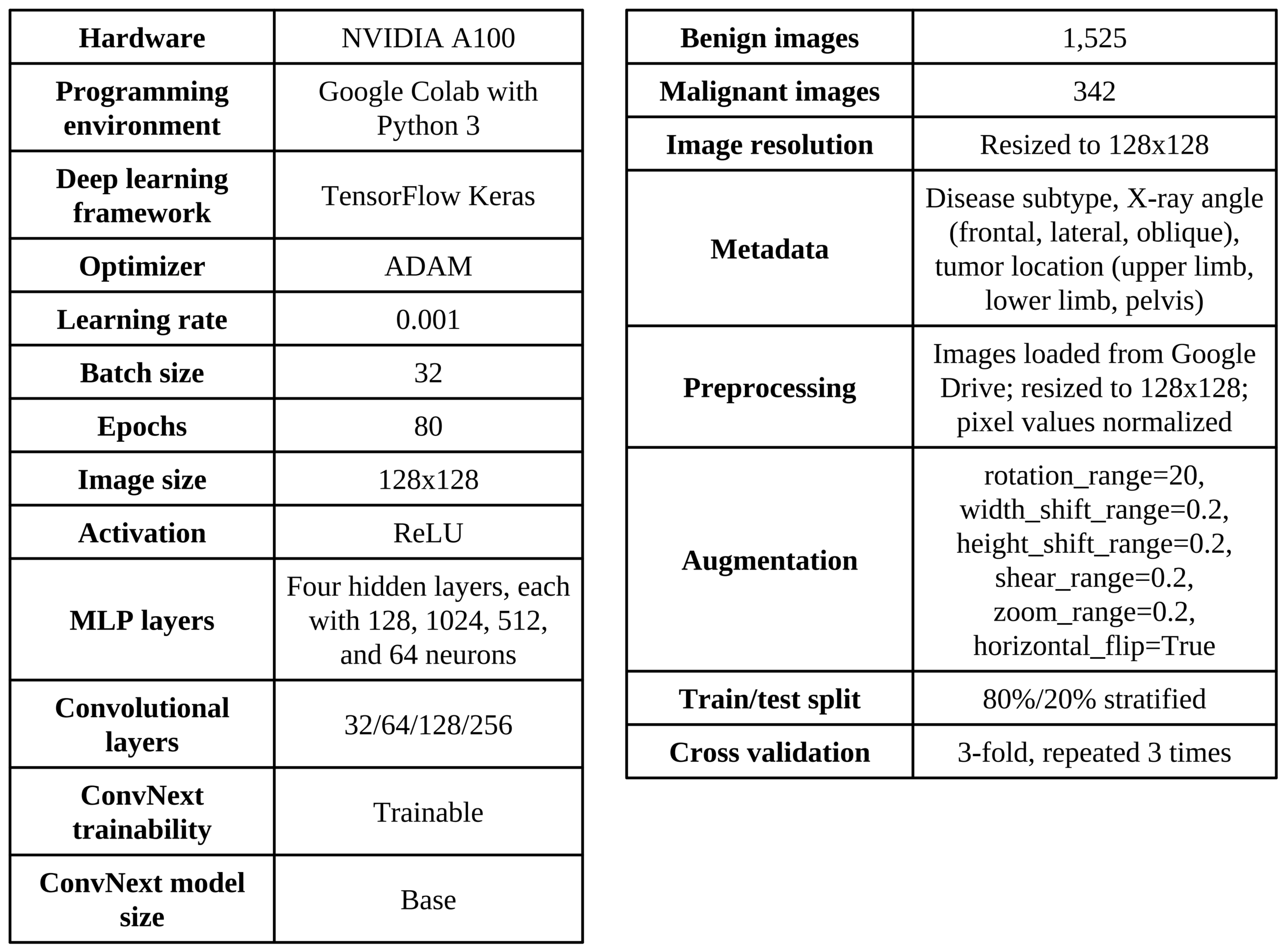
We tested all three models on Google Colab and used Python 3 as the runtime environment. For the hardware accelerator, we chose either CPU or A100 GPU. The dataset used for testing bone tumor classification is called BTXRD^17,18. It comprises 3,746 bone images, of which 1,879 are normal and 1,867 are tumor images. Not all images have tumors. Therefore, we wrote a Python script to train our AI models exclusively on images with tumors, including 1,525 benign and 342 malignant cases. The BTXRD dataset additionally provides a metadata spreadsheet that provides training labels in addition to other information, including the type of disease (e.g., osteosarcoma, osteochondroma, multiple osteochondromas, etc.), the angle of the X-ray (frontal, lateral, oblique), and the location of the tumor (upper limb, lower limb, pelvis). We stored all of the tumor images from the BTXRD dataset on Google Drive, and used Tensorflow with Keras and Scikit-learn packages to build the AI models. Unless otherwise specified, the default setting of our training are as follows: The number of epochs is set to 80, and the resolution of images is 128×128. The batch size is 32. We use 80% and 20% of the data for training and testing. Unless otherwise mentioned, each run is repeated three times and the average is reported. In Table 2, we list the default experimental configuration for three models.

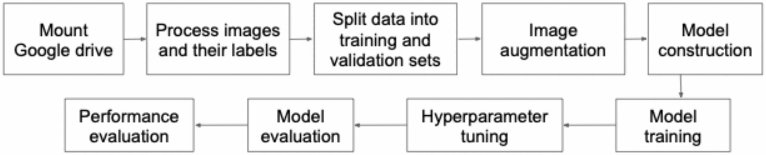
Figure 2 shows our experimental pipeline that consists of 1) mounting Google Drive for data loading, 2) processing all images as well as their labels, 3) splitting data into training and validation sets, 4) augmenting images since the number of malignant cases is low, 5) model construction, 6) model training, 7) hyperparameter tuning, 8) model evaluation, and 9) final performance evaluation. For the best outcomes of each model, hyperparameter tuning and evaluation will be repeatedly conducted.

We put the implementation (Google Colab Python code), which includes preprocessing and hyperparameters, on GitHub (https://github.com/KeithShi/bonetumor.git). The model weights are uploaded to HuggingFace (https://huggingface.co/Keithshi/mlp-bone).

Results

Figure 3 shows the test accuracy of MLP. In particular, in Figure 3(a), we vary the total number of training epochs to assess the convergence behavior of the model. Overall, the accuracy is relatively insensitive to the training time after 10 epochs. The reason for the fast convergence is that MLP, unlike CNN or ConvNext which both use sophisticated filters to extract features, has a relatively simple architecture with fewer model parameters. As a result, MLP can be trained and converge to the maximum accuracy quickly. Compared with CNN and ConvNext, MLP is expected to be less effective at extracting cancer-related features. In Figure 3(b), we further test different MLP network architectures and assess their impact on the overall accuracy. In particular, we test the following four designs: 1) a single layer with 128 neurons; 2) the same 128-neuron layer with an addition of a 1024-neuron layer (i.e., the “128/1024” case); 3) the same two layers with an addition of another 512-neuron layer (i.e., the “128/1024/512” case); and 4) the same three layers with an addition of another 64-neuron layer (i.e., the “128/1024/512/64” case). As shown in Figure 3(b), the number of layers does not significantly affect the overall accuracy. This behavior is attributed to the structure of MLP, which uses fully connected layers that treat the input as a flat set of numbers rather than 2D images. As a result, MLP learns most of its information in the first layer, so simply adding more layers does not significantly improve accuracy. Overall, despite its relatively lower accuracy, MLP remains a solid choice among the AI models we tested due to its low training cost (as shown in Figure 5(g)).

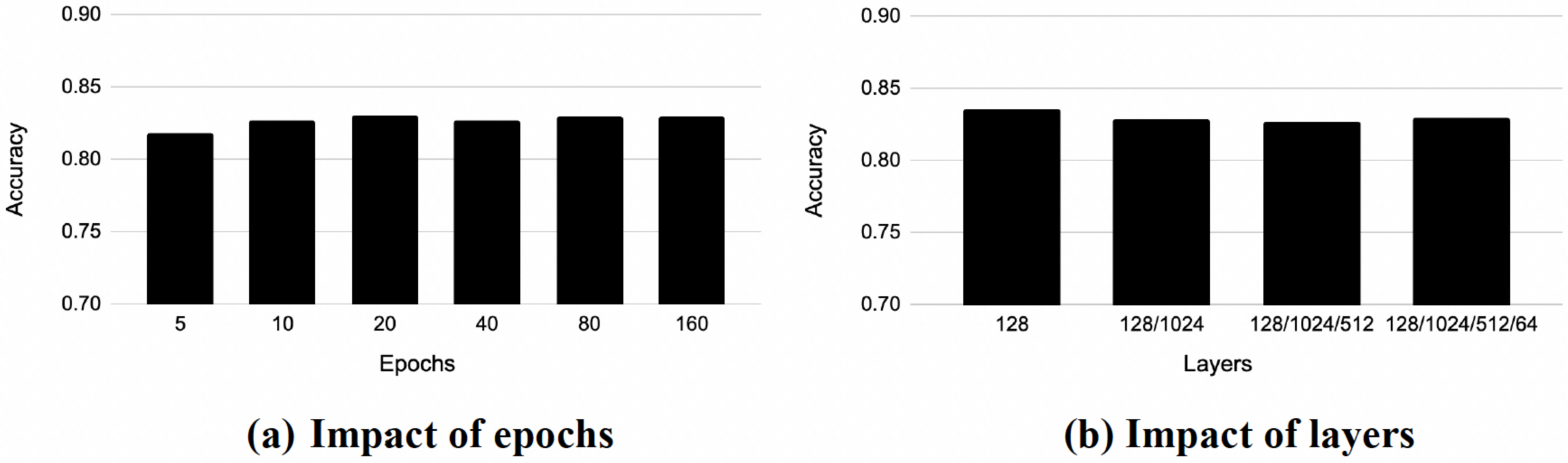
Figure 4 evaluates the accuracy of the CNN. In Figure 4(a), we again vary the number of epochs from 10 to 160. In contrast to MLP, CNN shows a steady improvement in accuracy till 40 epochs, and the trend flattens afterward. The more pronounced improvement in accuracy versus epochs is due to the higher complexity of CNNs (e.g., the use of filters) in capturing features, and therefore, longer epochs are needed to train a larger parameter space. In Figure 4(b), we test different configurations of convolution layers: 1) a single 2D convolutional layer with 32 filters, with each filter being 3×3 (i.e., the “32” case); 2) two layers, with an added layer of 64 filters (i.e., the “32/64” case); 3) three layers, with an added layer of 128 filters (i.e., the “32/64/128” case); 4) four layers, with an added layer of 256 filters (i.e., the “32/64/128/256” case); 5) five layers, with an added layer of 512 filters (i.e., the “32/64/128/256/512” case). Overall, as the complexity of CNN increases, a steady improvement in accuracy is observed.

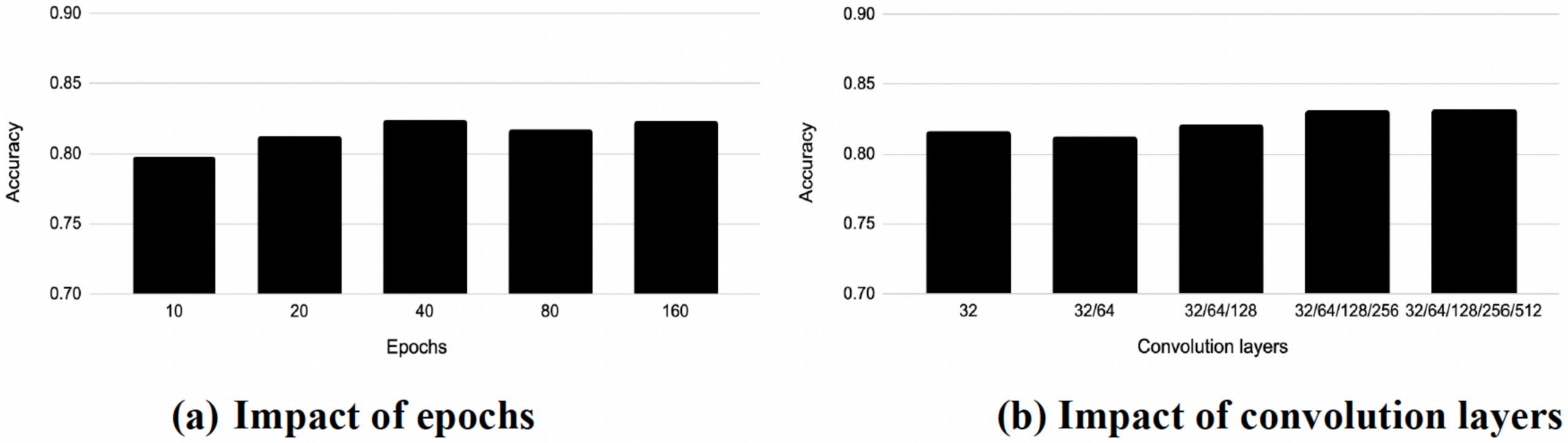
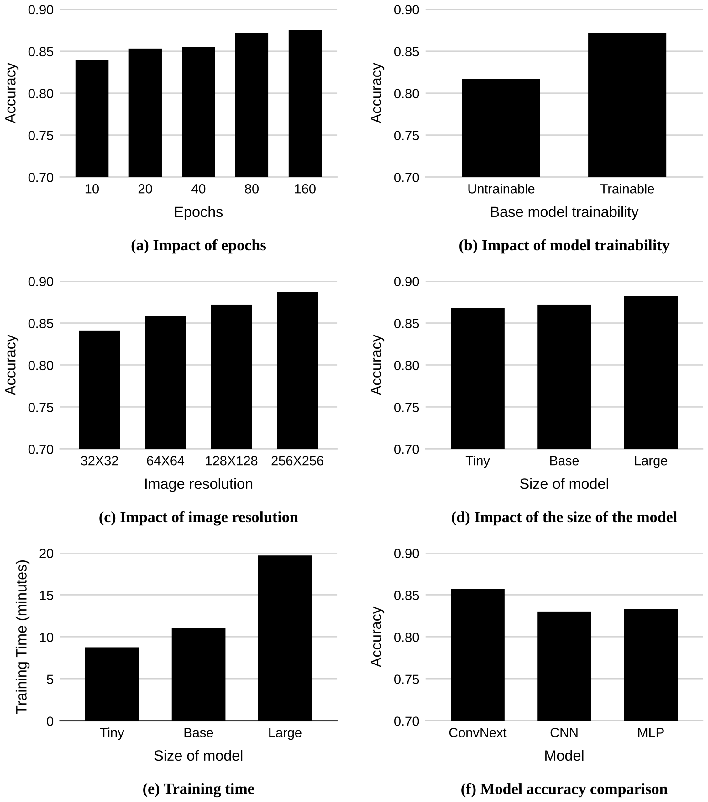
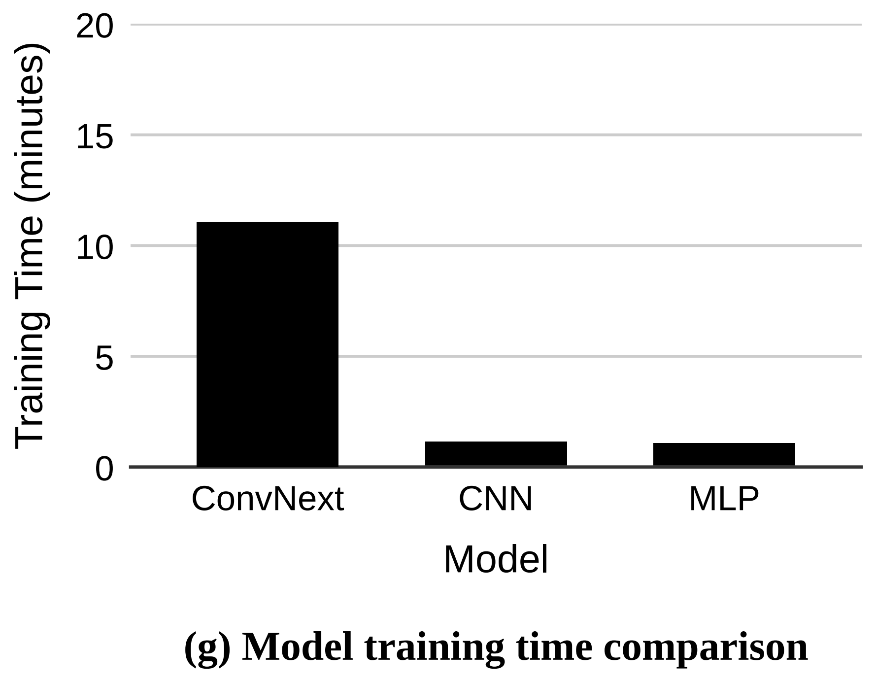
Figure 5 evaluates the performance of ConvNext under different configurations. In particular, Figure 5(a) tests the effect the epoch has on accuracy. Compared to the earlier results of MLP and CNN, a more pronounced effect of epoch on accuracy is observed. This is because ConvNext is a highly complex, fine-tuned model and can therefore better capture local features in the data. With more training epochs, the large parameter space can be better adjusted to minimize the cost function. Figure 5(b) compares the two training scenarios in which the base model parameter is frozen (here referred to as “untrainable”) and unfrozen (“trainable”). When the base model parameter is untrainable, only the two dense layers after the convolutional base are trainable. In contrast, when the base model parameter is trainable, the parameters of all layers are trainable. The results show that the trainable configuration achieves much higher accuracy than the untrainable one. Figure 5(c) studies the impact of the image resolution. In the experiment, we vary the image size from 32×32 to 256×256. It is shown that the accuracy increases with model resolution, albeit at a higher training cost. In Figure 5(d), we vary the size of the ConvNext model, i.e., tiny, base, and large. These variants share a similar architecture but differ in scale and size. The tiny model is the smallest and most shallow, with approximately 28 million parameters. The base model adds more layers, bringing the parameter count to approximately 89 million, while the large model makes the network wider with more channels at each stage, reaching approximately 198 million parameters. It is observed that as the model size increases, so does its accuracy, with the largest model achieving the highest accuracy. Furthermore, in Figure 5(e), we compare the training times of the three ConvNeXt variants. As expected, the tiny model has the shortest training time, and the large model has the longest training time. When comparing Figure 5(d) and Figure 5(e), we can see that the tiny model has lower accuracy but takes significantly less time to train. More importantly, because it has fewer parameters, it consumes less memory, making it a good choice for resource-constrained computer systems for training or inference. In Figure 5(f), we compare the test accuracy of ConvNext, CNN, and MLP; because ConvNext is a highly optimized architecture, it achieves the highest accuracy. In Figure 5(g), we further compare the training of all these models. Clearly, the base ConvNext has an order-of-magnitude higher training cost than the other two models. With regard to the model complexity, we further describe the model size and memory consumption below.

• MLP: 2.2 Million parameters with 8.8 MB memory consumption
• CNN: 1 to 2 Million parameters with 4 to 8 MB memory consumption
• ConvNeXt (Tiny): 28 Million parameters with 112 MB memory consumption
• ConvNeXt (Base): 89 Million parameters with 356 MB memory consumption
• ConvNeXt (Large): 198 Million parameters with 792 MB memory consumption

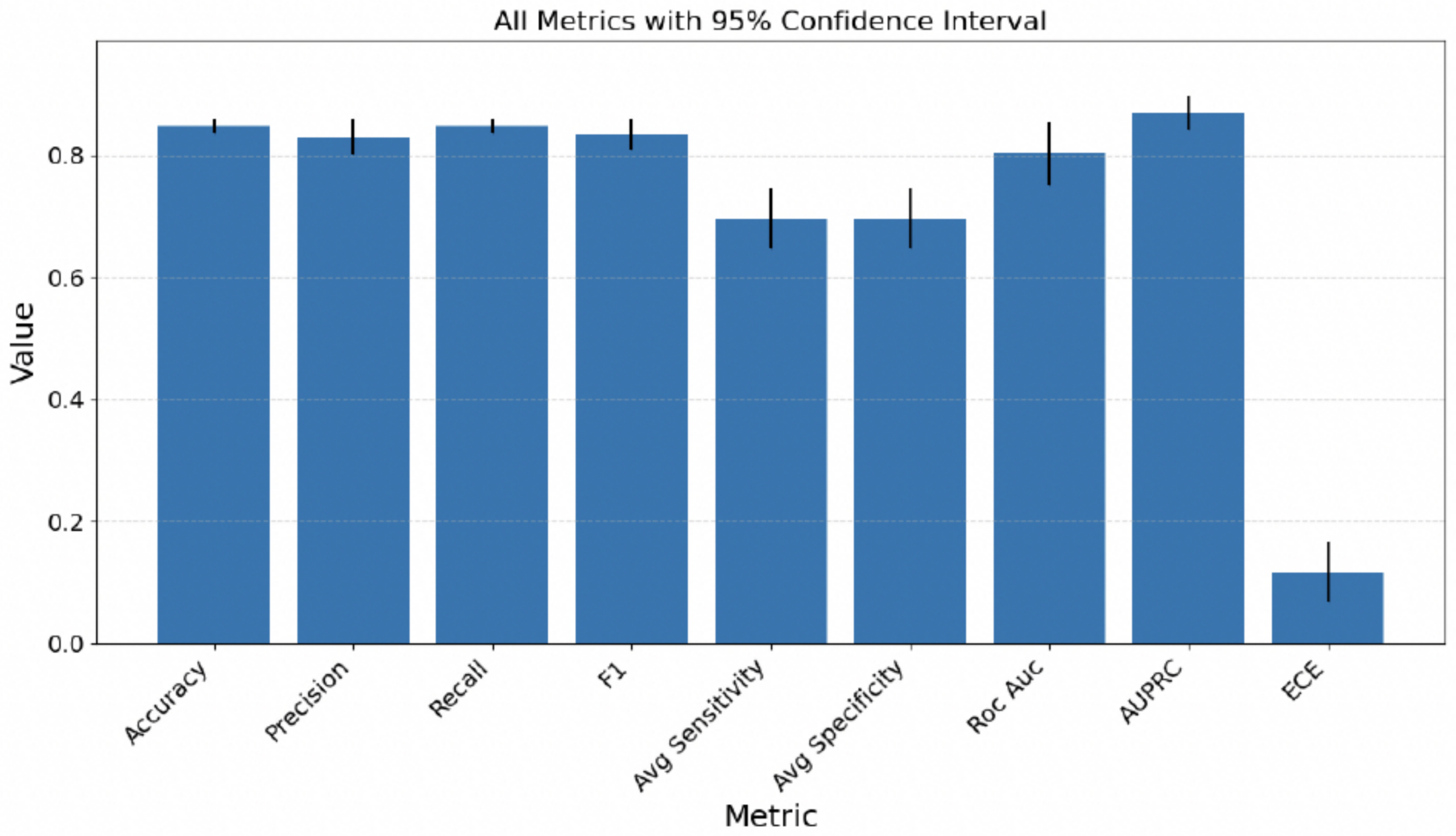
Given the small number of images that are labeled as cancerous, we further perform repeated stratified k-fold cross-validation in Figure 6, where both the number of folds and the number of times to repeat the experiment are set to 3. Higher values of these parameters would yield more robust results but require significantly longer training times, which would not allow us to complete this work within a realistic time frame and monetary cost. In Figure 6, we show the 95% confidence interval for all metrics for ConvNext.

Model	Accuracy	Precision	Recall	F1	Sensitivity	Specificity	Roc Auc
MLP	0.82	0.73	0.82	0.77	0.54	0.54	0.60
CNN	0.81	0.80	0.80	0.80	0.66	0.66	0.75
ConvNext	0.85	0.84	0.85	0.84	0.70	0.70	0.82

Model	Confusion matrix
MLP	[300  6] [ 58 10]
CNN	[274 32]  [37   31]
ConvNext	[289 17]  [37   31]

To address potential evaluation bias caused by class imbalance in BTXRD, all three architectures were evaluated across a comprehensive set of performance metrics, including sensitivity, specificity, precision, recall, F1-score, ROC-AUC, and confusion matrices. Table 3 summarizes the performance across models, while Table 4 details the corresponding confusion matrices.

Evaluating models solely on overall accuracy can create a false impression of diagnostic effectiveness. Although the MLP achieved an overall accuracy of 82%, its confusion matrix shows a severe bias toward the majority class: it correctly identified only 10 out of 68 malignant tumors (a true positive rate of only 14.7%), misclassifying the remaining 58 malignant cases as benign. Both spatial feature extraction architectures demonstrated significantly improved class balance. The custom CNN achieved an accuracy of 81%, an F1-score of 0.80, and an ROC-AUC of 0.75, correctly classifying 31 malignant cases. ConvNeXt achieved the strongest overall performance, with an accuracy of 85%, an F1-score of 0.84, and an ROC-AUC of 0.82. ConvNeXt matched the CNN’s malignant classification capacity (31 true positives) while reducing false positives by nearly half (17 vs. 32), illustrating the benefit of modern vision architectures when handling imbalanced medical datasets. From Tables 5 to 7, we further break down the performance of all three models into benign and cancerous classes due to the imbalanced nature of the dataset. It is clear that ConvNext can perform better than the other two models for the cancerous class.

Class	Precision	Recall	F1	Sensitivity	Specificity	Roc Auc	AUPRC	Calibration
Benign	0.86	0.92	0.89	0.92	0.31	0.65	0.87	0.14
Cancerous	0.47	0.31	0.37	0.31	0.92	0.65	0.37	0.14

Class	Precision	Recall	F1	Sensitivity	Specificity	Roc Auc	AUPRC	Calibration
Benign	0.86	0.94	0.90	0.94	0.34	0.74	0.92	0.14
Cancerous	0.56	0.34	0.42	0.34	0.94	0.74	0.47	0.14

Class	Precision	Recall	F1	Sensitivity	Specificity	Roc Auc	AUPRC	Calibration
Benign	0.88	0.96	0.91	0.96	0.40	0.80	0.94	0.1093
Cancerous	0.67	0.40	0.50	0.40	0.96	0.80	0.58	0.1093

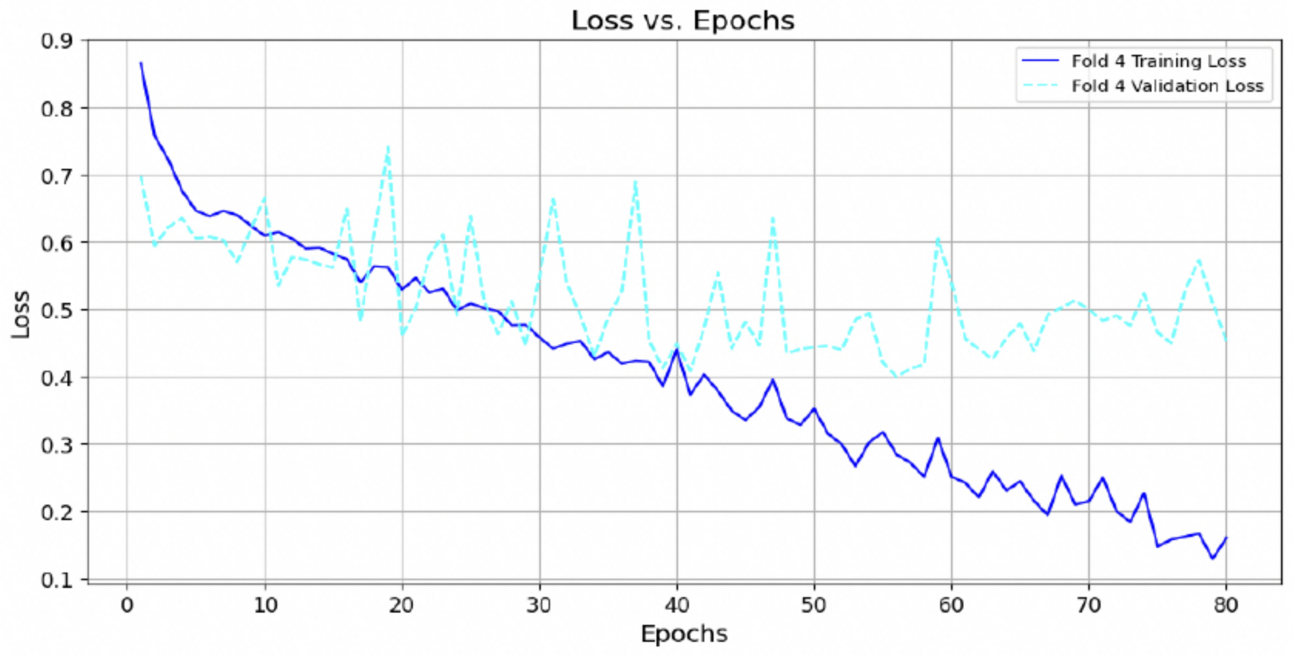
In Figure 7, we evaluate the training and validation loss across time for fold 4 for ConvNext. It is illustrated the validation loss improves as the training loss is reduced by the model till 40 epochs. After that, the validation loss stabilizes, showing that the model is neither overfit or underfit. In Figure 8, we generate the heatmap for a malignant image using Grad-CAM,and verify that our trained model can focus on the region that potentially has a malignant tumor. In particular, regions with warm colors indicate high-importance regions, while regions with cool colors indicate low-importance regions.

Discussion. This work is envisioned to help assist radiologists by classifying tumors as benign or malignant, rather than completely replace human diagnosis. With AI capabilities, each X-ray image must still be examined by a radiologist manually. With this work, we can rapidly pre-screen patients so that those who are classified as malignant can be expedited for human verification/treatment as compared to those who are classified as benign. Thus, those false positive cases can be eliminated by human verification later. For those that are false negatives, unfortunately, they will not be prioritized but will be verified by radiologists later, thus consuming the same amount of time as the current practice where only radiologists are involved.

Our base ConvNext model achieved 85.5% accuracy and ROC-AUC of 82.2% on BTXRD. Wang et al. achieved 88.1% (internal) and 89.5% (external) accuracy using an ensemble of EfficientNet,ViT, and Swin Transformer fused with clinical features across a larger multicenter cohort⁸. Von Schacky et al. reported 80.2% accuracy on an external test set using a multitask CNN⁶. Song et al.’s multimodal transformer achieved AUC of 0.847 (internal) and 0.782 (external) combining X-ray, CT, and MRI⁵; our AUC of 0.822 falls within this range using X-ray alone, suggesting a well-tuned single-modality CNN can be competitive with more complex multimodal pipeline, though this comparison should be read cautiously given differences in dataset and validation strategy.

By contrast, histopathology-based studies report substantially higher accuracies, generally above 95%^9,10,13, likely reflecting task difficulty rather than model quality: histopathology captures direct cellular-level malignancy evidence, while radiographs capture only more relevant to early, non-invasive pre-screening, even with a lower achievable accuracy.

Methodologically, the strongest prior radiograph studies used multicenter data with external validation and ensembles of multiple backbones^5,8 whereas we evaluate a single architecture on a single-center dataset with only internal cross-validation. Some of the residual performance gap may therefore reflect these methodological differences rather than architecture choice alone, reinforcing the external validation limitation discussed in Conclusions and Future Work.

Conclusions and Future Work

The three AI models – MLP, CNN, and ConvNext- used in this study achieved accuracy rates as high as 89% for the BTXRD dataset, displaying the potential for using AI in bone tumor classification. These findings show that each AI model has their own pros and cons. MLP is the least sensitive to hyperparameter changes, with the lowest accuracy. Despite this, MLP achieves the fastest and most efficient training time. CNN showed more sensitivity to hyperparameters and achieved slightly higher accuracy. Overall, ConvNext achieves the highest accuracy among the three models, albeit at the cost of significantly longer training time.

However, this study is limited in scope, as it evaluates only three AI models and focuses exclusively on bone tumor classification using BTXRD only. In addition, the BTXRD dataset used to train the three models is considerably imbalanced, with fewer malignant cases than benign. This, in turn, means that the models have not been fully tested across a wide and representative range of cases, which may, in some cases, reduce accuracy. Future research should explore larger, more balanced datasets, a broader range of AI architectures, and the application of these models to other types of X-ray diagnoses beyond bone cancer.

We would note, however, that our study was designed and presented as a small prototype for method comparison among MLP, CNN, and ConvNext architectures using BTXRD. It is not intended for developing a clinically validated diagnostic tool, which requires significant engineering efforts that are beyond the scope of a high-school student research project. In addition, a full investigation of scanner variability, multi-site generalizability, demographic diversity, and clinical integration would require access to significantly more imaging data and clinical infrastructure, which were both not available at this time. We believe such analyses are better suited to an independent, follow-up study that specifically focuses on the practical aspects of using AI models for bone tumor classification.

Since our dataset is small and imbalanced with only 342 malignant cases, further splitting the data into validation and test may result in fluctuating results. On the other hand, how to choose the test data remains a question for us–an inappropriate choice of test data may artificially boost/degrade the results of the model significantly, due to the small scale of the malignant data and some of the images can be from the same patients. Given these limitations, the three-way train/validation/test split is left for future study.

All performance metrics come from a single held-out 80/20 train-test split drawn from the same dataset and source institution. No independent external set from a different hospital, population, or imaging system was evaluated. This contrasts with recent bone tumor classification studies that report both internal and external test performance^5,8, now considered a stronger standard for demonstrating generalizability. Without external validation, the reported 89% accuracy may partly reflect dataset-specific characteristics rather than generalizable performance.

This study does not assess performance on X-ray images acquired with different scanner manufacturers, protocols, or resolutions than those in BTXRD. Acquisition variability across clinical sites is a well-documented source of performance degradation for learning models in radiology. ConvNext’s strong performance here, achieved by fine-tuning pretrained weights, does not by itself establish that learned features transfer robustly to X-ray images acquired under different clinical conditions.

Future work, building on these limitations, should identify the following concrete steps: evaluating these models on larger, more balanced datasets, potentially through multi-institutional data sharing or targeted augmentation of the malignant class; external validation on at least one independent dataset from a different institution and/or imaging system; systematic testing of robustness to scanner and protocol variability; and prospective multi-centre clinical validation, comparing model predictions against radiologist interpretation and histopathological ground truth in real workflows, following the design of recent randomized and multi-reader radiology AI studies^1,32. Such a trial would establish not only diagnostic accuracy but clinical utility, a distinction that has produced mixed results even for more mature applications, such as chest X-ray triage.

References

1. Woznitza, N., Smith, L., Rawlinson, J. et al. AI-based chest X-ray prioritization in the lung cancer diagnostic pathway: the LungIMPACT randomized controlled trial. Nat Med (2026 [↩] [↩]
2. López Alcolea J, et al.. Diagnostic Performance of Artificial Intelligence in Chest Radiographs Referred from the Emergency Department. Diagnostics (Basel). 2024 Nov 18;14(22):2592. doi: 10.3390/diagnostics14222592. PMID: 39594258; PMCID: PMC11592727 [↩]
3. Willenbring TJ, Papa SM, Mann KA, Cavallaro SM, Damron TA. Classifications for radiographic evaluation of radiolucent bone lesions have poor inter- and intra-observer agreement. BMC Musculoskelet Disord. 2025;26(1):649. doi:10.1186/s12891-025-08815-5 [↩]
4. Yuan B, Hu Y, Liang Y, Zhu Y, Zhang L, Cai S, Peng R, Wang X, Yang Z, Hu J. Comparative analysis of convolutional neural networks and transformer architectures for breast cancer histopathological image classification. Front Med. 2025;12:1606336 [↩] [↩]
5. Song L, Li C, Tan L, Wang M, Chen X, Ye Q, Li S, Zhang R, Zeng Q, Xie Z, Yang W, Zhao Y. A deep learning model to enhance the classification of primary bone tumors based on incomplete multimodal images in X-ray, CT, and MRI. Cancer Imaging. 2024;24(1):135 [↩] [↩] [↩] [↩] [↩]
6. Von Schacky CE, Wilhelm NJ, Schäfer VS, Leonhardt Y, Gassert FG, Foreman SC, Gassert FT, Jung M, Jungmann PM, Russe MF, et al. Multitask deep learning for segmentation and classification of primary bone tumors on radiographs. Radiology. 2021;301(2):398-406 [↩] [↩] [↩]
7. Dalai SS, Ranjan Sahu BJ, Rautaray J, Khan MI, Jabr BA, Ali YA. Automated Bone Cancer Detection Using Deep Learning on X-Ray Images. Surg Innov. 2025;32(2):94-108 [↩] [↩]
8. Wang H, He Y, Wan L, Li C, Li Z, Li Z, Xu H, Tu C. Deep learning models in classifying primary bone tumors and bone infections based on radiographs. npj Precis Oncol. 2025;9:72 [↩] [↩] [↩] [↩] [↩]
9. Borji A, Kronreif G, Angermayr B, Hatamikia S. Advanced hybrid deep learning model for enhanced evaluation of osteosarcoma histopathology images. Front Med. 2025;12:1555907 [↩] [↩] [↩]
10. Walid MAA, Mollick S, Shill PC, Baowaly MK, Islam MR, Ahamad MM, Othman MA, Samad MA. Adapted Deep Ensemble Learning-Based Voting Classifier for Osteosarcoma Cancer Classification. Diagnostics. 2023;13(19):3155. doi:10.3390/diagnostics13193155 [↩] [↩] [↩]
11. Li X, Ding R, Wang Q, Yang Z, Duan X, Sun Y, Liu A. EENet: Application of convolutional neural network-based deep learning methods in bone tumor pathological diagnosis. Int J Imaging Syst Technol. 2024;34(3):e23082 [↩] [↩] [↩]
12. Sampath K, Rajagopal S, Chintanpalli A. A comparative analysis of CNN-based deep learning architectures for early diagnosis of bone cancer using CT images. 2024 [↩] [↩]
13. Aziz MT, Mahmud SMH, Elahe MF, Jahan H, Rahman MH, Nandi D, et al. A novel hybrid approach for classifying osteosarcoma using deep feature extraction and multilayer perceptron. Diagnostics. 2023;13(12):2106. doi:10.3390/diagnostics13122106 [↩] [↩] [↩]
14. Song L, et al. Development of the interpretable typing prediction model for osteosarcoma and chondrosarcoma based on machine learning and radiomics: a multicenter retrospective study. Front Med. 2024;11. doi:10.3389/fmed.2024.1497309 [↩] [↩]
15. Anisuzzaman DM, Barzekar H, Tong L, Luo J, Yu Z. A deep learning study on osteosarcoma detection from histological images. Biomed Signal Process Control. 2021;69:102931. doi:10.1016/j.bspc.2021.102931 [↩] [↩]
16. Papageorgiou PS, et al. Artificial Intelligence in Primary Malignant Bone Tumor Imaging: A Narrative Review. Diagnostics (Basel). 2025 Jul 4;15(13):1714. doi: 10.3390/diagnostics15131714. PMID: 40647712; PMCID: PMC12248882 [↩]
17. Yao S, Huang Y, Wang X, Zhang Y, Paixao IC, Wang Z, Chai CL, Wang H, Lu D, Webb GI, Li S, Guo Y, Chen Q, Song J. A Radiograph Dataset for the Classification, Localization, and Segmentation of Primary Bone Tumors. Sci Data. 2025 Jan 16;12(1):88 [↩] [↩]
18. BTXRD dataset, 10.6084/m9.figshare.27865398 [↩] [↩]
19. Setiawan D, Karnyoto AS, Intan I, Pardamean B. ConvNeXt Model for Breast Cancer Image Classification. In: 2024 6th International Conference on Cybernetics and Intelligent System (ICORIS). 2024. doi:10.1109/ICORIS63540.2024.10903832 [↩]
20. Lu G, Tian R, Yang W, Liu R, Liu D, Xiang Z, Zhang G. Deep learning radiomics based on multimodal imaging for distinguishing benign and malignant breast tumours. Front Med. 2024 [↩]
21. Giourga M, Petropoulos I, Stavros S, et al. A Deep Learning Approach for Classifying Benign, Malignant, and Borderline Ovarian Tumors Using Convolutional Neural Networks and Generative Adversarial Networks. Med Sci (Basel). 2026;14(1):89. doi:10.3390/medsci14010089 [↩]
22. Liu M, et al. A multilayer perceptron-based model applied to histopathology image classification of lung adenocarcinoma subtypes. Front Oncol. 2023;13:1172234 [↩]
23. Zhou Z, Islam MT, Xing L. Multibranch CNN With MLP-Mixer-Based Feature Exploration for High-Performance Disease Diagnosis. IEEE Trans Neural Netw Learn Syst. 2024 Jun;35(6):7351-7362. doi: 10.1109/TNNLS.2023.3250490. Epub 2024 Jun 3. PMID: 37028335; PMCID: PMC11779602 [↩]
24. Kumar A, Patel P, Robert D, Kumar S, Khetani A, Reddy B, Srivastava A. Accuracy of an artificial intelligence-enabled diagnostic assistance device in recognizing normal chest radiographs: a service evaluation. BJR Open. 2024. doi:10.1093/bjro/tzae029 [↩]
25. Zhao D, et al. A. Diagnostic accuracy of artificial intelligence-assisted radiology assessment of cancer: a systematic review. BJR Artif Intell. 2025;2(1):ubaf016. doi:10.1093/bjrai/ubaf016 [↩]
26. Walsh R, Tardy M. A Comparison of Techniques for Class Imbalance in Deep Learning Classification of Breast Cancer. Diagnostics. 2023;13(1):67. doi:10.3390/diagnostics13010067 [↩]
27. Yoshitsugu K, Kishimoto K, Takemura T. Improving the Sensitivity of Unbalanced Medical Image Classification by Random Up-sampling Numerical Features. In: Proc. 2024 6th Int. Conf. on Intelligent Medicine and Image Processing (IMIP 2024). 2024 [↩]
28. Hellín CJ, Olmedo AA, Valledor A, Gómez J, López-Benítez M, Tayebi A. Unraveling the Impact of Class Imbalance on Deep-Learning Models for Medical Image Classification. Applied Sciences. 2024; 14(8):3419. https://doi.org/10.3390/app14083419 [↩]
29. Gao L, Zhang L, Liu C, Wu S. Handling imbalanced medical image data: A deep-learning-based one-class classification approach. Artif Intell Med. 2020 Aug;108:101935. doi: 10.1016/j.artmed.2020.101935. Epub 2020 Aug 7 [↩]
30. Bani Baker Q, Hammad M, Al-Smadi M, Al-Jarrah H, Al-Hamouri R, Al-Zboon SA. Enhanced COVID-19 Detection from X-ray Images with Convolutional Neural Network and Transfer Learning. J Imaging. 2024 Oct 13;10(10):250 [↩]
31. Almutaani M, Turki T, Taguchi YH. Novel large empirical study of deep transfer learning for COVID-19 classification based on CT and X-ray images. Sci Rep. 2024 Nov 3;14(1):26520 [↩]
32. Guo L, et al. Deep Learning for Chest X-ray Diagnosis: Competition Between Radiologists with or Without Artificial Intelligence Assistance. J Digit Imaging Inform Med. 2024;37:922-934. doi:10.1007/s10278-024-00990-6 [↩]