Controlled Evaluation of Transfer Learning for Brain Tumor MRI Classification and Detection

Abstract

Background/Objective: Transfer learning is widely used in medical imaging, but many studies compare models that also differ in architecture or training procedure. This makes it difficult to determine how much of the performance difference comes from pretraining itself. This study tested if pretraining improves brain tumor MRI classification and detection when architecture, data split, and evaluation are held constant.
Methods: A public brain MRI dataset containing glioma, meningioma, pituitary tumor, and no-tumor images was screened before training, validation, and test sets were created. Identical ResNet-50 classifiers started from either ImageNet-pretrained or random weights and were trained on the same MRI images. A third classifier kept the pretrained ResNet-50 backbone fixed and trained only the final layer. Detection used matched Faster R-CNN ResNet-50-FPN models with pretrained or reinitialized weights. Final comparisons used three seeds.
Results: ImageNet fine-tuning achieved a macro-F1 of 0.99, compared with 0.96 for random training and 0.93 for the frozen-feature model. With 10% of the training data, macro-F1 was 0.89 for pretrained models and 0.59 for random models. Pretrained detection achieved an mAP of 0.69 versus 0.31 after random initialization.
Conclusions: Pretraining improved both tasks in this dataset, with the largest classification benefit when labeled data were limited. Full fine-tuning outperformed both random training and fixed ImageNet features. Missing patient identifiers, differences in image sources, and the lack of an independent external test set limit conclusions about clinical performance.

Keywords: brain tumor MRI; transfer learning; ResNet-50; Faster R-CNN; data leakage; RadImageNet; limited training data; robustness

Introduction

Magnetic resonance imaging (MRI) is widely used to examine brain tumors because it produces detailed images of soft tissue without using X-rays. Brain tumors can differ in type, location, appearance, and behavior, so diagnosis cannot rely on a single visual feature.¹ Computer models have therefore been studied for tasks such as identifying tumor type, locating tumors, and marking the tumor area in an image.^2,3 One common approach is transfer learning, where a model first learns from a large image dataset and is then trained further on a smaller medical dataset. This is useful because medical datasets are often much smaller than the image collections used to train modern neural networks. Several studies have reported strong brain tumor MRI classification results using CNN-based approaches, including transfer learning and ensemble deep features.^4,5,6,7,8 Other studies have examined active learning, data augmentation, transfer learning, and ensemble CNN approaches for brain tumor MRI classification.^{9,10,11,12,13} More recent studies have also reported high accuracy for classification problems that separate glioma, meningioma, pituitary tumor, and no-tumor images.^14,15,16,17 

However, these studies do not always show how much of the improvement comes from pretraining itself. In some comparisons, the pretrained model and the model trained from random weights also differ in architecture, training schedule, or data split. This makes it difficult to know if pretraining is the main reason for the performance difference. Studies in medical imaging have found that pretrained models can outperform randomly initialized models, especially when training data are limited, but the size of this benefit varies across tasks.^18,19,20,21 Pretraining on medical images has also been explored. RadImageNet, for example, was built from more than one million radiology images and was designed to provide features that may transfer well to medical imaging tasks.²² Other work has examined medical-image pretraining and learning methods that do not depend on standard ImageNet labels.^23,24,25

The same question also applies to tumor detection. Classification asks what type of tumor is present in an image, while detection asks the model to identify the tumor and locate it with a bounding box. Previous studies have used deep learning for brain tumor detection and for marking tumor regions in MRI.^26,27 Because detection requires both identification and location, pretrained and randomly initialized models should be compared using the same detector structure and evaluation method. ResNet-50 and Faster R-CNN are widely used for image classification and object detection and provide a clear way to make this comparison.^28,29,30,31

This study asks a simple question: when model architecture, data split, and evaluation are kept the same, does pretraining improve brain tumor MRI classification and detection? For classification, identical ResNet-50 models were trained on the same MRI images starting from either ImageNet-pretrained or random weights. A third model kept the pretrained ResNet-50 features fixed and trained only the final classification layer. This tested if fixed pretrained features were useful on their own and how much further training on MRI images improved performance. For detection, identical Faster R-CNN ResNet-50-FPN models were trained from either pretrained or random weights.

The study also examined when pretraining was most useful. Classification was repeated with smaller training sets, ImageNet pretraining was compared with RadImageNet pretraining, and model performance was tested after changes in blur, contrast, and image noise. The dataset was also checked for labeling problems and duplicate images before the final training, validation, and test sets were created. Because patient identifiers and complete image-source information were not available, the study is intended as a controlled comparison of training methods on a public dataset rather than a test of clinical performance.

Methods

Research design

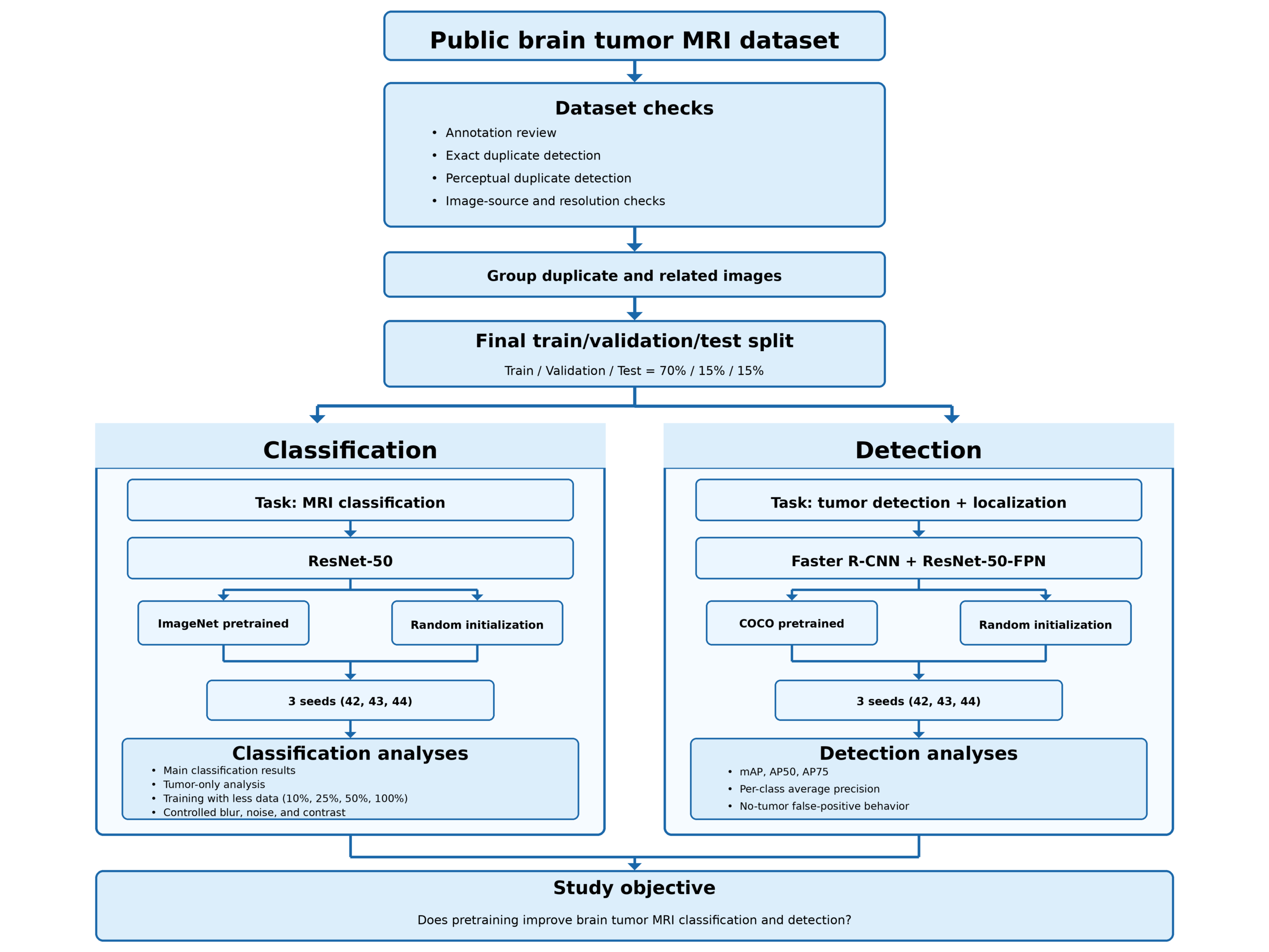
This study used the public MRI for Brain Tumor with Bounding Boxes dataset.³² Before training, the dataset was checked for labeling errors, duplicate images, and other image differences that could affect the results.

The final dataset was divided into training, validation, and test sets. The training set was used to train the models, the validation set was used to choose model settings, and the test set was used only for the final evaluation.

For classification, both main models used the same ResNet-50 architecture. One started from ImageNet-pretrained weights, while the other started from random weights. Both were trained on the same MRI training set. A third ResNet-50 model kept the pretrained image features fixed and trained only the final classification layer.

For detection, both models used the same Faster R-CNN ResNet-50-FPN architecture. One started from COCO-pretrained weights, while the other started from random weights.

Final comparisons were repeated with three random seeds: 42, 43, and 44. The overall study design and data preparation process are shown in Figure 1.

Dataset preparation

The downloaded dataset listed 5,249 images labeled as glioma, meningioma, pituitary tumor, or no tumor. Two images were missing, leaving 5,247 available images.

The labels and tumor boxes were checked before training. Of the available images, 4,976 had consistent labels, 257 contained mixed class labels, 15 contained an incorrect class label, and one tumor image had no tumor box. Images with mixed or incorrect labels were removed. The tumor image without a box was kept for classification but removed from detection.

Exact duplicate images were identified using SHA-256 file hashes. This found 1,228 duplicate groups containing 2,564 images, including 213 groups that appeared in both the original training and validation folders.

Because exact file matching cannot identify images that were resaved, compressed differently, or slightly changed, near-duplicate images were also checked using perceptual hashing, grayscale image comparisons, and pixel-correlation checks. Identical or nearly identical images were placed in the same group so they could not appear in different training, validation, or test sets.

After these checks, 3,710 images remained for classification and 3,573 for detection. The final sample sizes for each split are provided in Table 1.

Task / split	Glioma	Meningioma	No tumor	Pituitary	Total
Classification: train	732	727	419	718	2,596
Classification: validation	157	156	90	154	557
Classification: test	157	156	90	154	557
Tumor-only classification: train	732	727	–	718	2,177
Tumor-only classification: validation	157	156	–	154	467
Tumor-only classification: test	157	156	–	154	467
Detection: train	723	697	419	656	2,495
Detection: validation	152	149	90	149	540
Detection: test	155	150	90	143	538

Image-source checks

The dataset did not provide reliable patient identifiers, complete MRI scanning information, or patient demographics. Images from the same patient therefore could not be guaranteed to remain in the same data split. The duplicate checks reduced image-level overlap but could not replace a true patient-level split.

The dataset also contained axial, coronal, and sagittal MRI views. These views were kept because complete view labels were not available.

Image size was strongly related to class. All glioma images examined in this analysis were 512 × 512 pixels, compared with 88.2% of meningioma images, 97.2% of pituitary images, and only 2.1% of no-tumor images. A simple model using image width, height, aspect ratio, and a 512-pixel-width indicator reached about 0.41 accuracy. This suggests that image properties unrelated to the tumor may provide information about the class.

A second public MRI dataset containing 5,941 images was considered for external testing. However, 2,113 images also appeared in the main dataset. Of the 889 images in its test set, 313 matched images in the main dataset, including 212 that matched main-dataset training images. Because the two datasets were not independent, the second dataset was not used for external testing.

Classification models and training

The two main classification models used identical ResNet-50 architectures.²⁸ The only starting difference was the model weights. One started from ImageNet-pretrained weights, while the other started from random weights. Both models were then fully trained on the same MRI training set.

Images were resized to 224 × 224 pixels. During training, images were horizontally flipped with a probability of 0.5. Validation and test images were not randomly flipped. All images used the same ImageNet normalization.

The classifiers were trained using cross-entropy loss, which penalizes the model when it assigns a low probability to the correct class:

Here, 𝑁 is the number of images, C is the number of classes, 𝑦𝑖𝑐 indicates the correct class, and 𝑝𝑖𝑐 is the predicted probability.

A third model tested the usefulness of pretrained ImageNet features without updating the feature extractor. The pretrained ResNet-50 was kept fixed, and only the final classification layer was trained. This model had 8,196 trainable parameters, compared with 23,516,228 in each fully trained ResNet-50.

Full training settings for the classification and detection models are provided in Table 2.

Setting	ImageNet fine-tuning	Random training	Frozen ImageNet	Detection pretrained	Detection random
Model	ResNet-50	ResNet-50	ResNet-50	Faster R-CNN ResNet-50-FPN	Faster R-CNN ResNet-50-FPN
Starting weights	ImageNet	Random	ImageNet	COCO	Random
Layers trained	All	All	Final layer only	All	All
Optimizer	AdamW	AdamW	AdamW	SGD	SGD
Batch Size	64	64	32	4	4
Weight decay	10⁻⁴	10⁻⁴	10⁻⁴	5 × 10⁻⁴	5 × 10⁻⁴
Selected learning rate	3 × 10⁻⁴	10⁻³	10⁻²	5 × 10⁻³	3 × 10⁻³
Maximum epochs	40	40	40	80	80
Early stopping patience	5	5	5	5	5
Final seeds	42, 43, 44	42, 43, 44	42, 43, 44	42, 43, 44	42, 43, 44

For the two main classifiers, learning rates of 10⁻⁴, 3 × 10⁻⁴, and 10⁻³ were tested. The best learning rate was chosen using validation macro-F1, giving 3 × 10⁻⁴ for the pretrained model and 10⁻³ for the random model.

For the frozen model, learning rates from 10⁻⁴ to 10⁻² were tested, with 10⁻² giving the highest validation macro-F1.

Both main classifiers used a ReduceLROnPlateau learning-rate scheduler with a factor of 0.3, patience of 2 epochs, and a minimum learning rate of 10⁻⁶.

Detection models and training 

Tumor detection used Faster R-CNN with a ResNet-50-FPN backbone.^29,30 Unlike classification, detection requires the model to identify the tumor type and draw a box around its location. 

No-tumor images were treated as images containing no tumor objects. They therefore contained no target boxes rather than an artificial “no tumor” box.

The two detector models used the same architecture and number of trainable parameters. Both detectors used the same FrozenBatchNorm configuration. The pretrained detector started from COCO-trained Faster R-CNN weights.³³ For the random detector, learned weights and stored normalization values were reset while the model architecture remained unchanged.

Both models were trained using stochastic gradient descent (SGD) with momentum 0.9 and weight decay 5 × 10⁻⁴. Learning rates of 10⁻³, 3 × 10⁻³, and 5 × 10⁻³ were tested using validation mAP. The selected learning rates were 5 × 10⁻³ for the pretrained detector and 3 × 10⁻³ for the random detector. Full training settings are provided in Table 2.

Faster R-CNN combines four losses that measure tumor classification, box location, object presence, and the quality of proposed tumor regions:

Additional classification experiments

Several additional experiments tested when pretraining was most useful.

First, classification was repeated after removing the no-tumor class. This tumor-only analysis tested if the main result remained when only glioma, meningioma, and pituitary tumors were included.

Second, the models were trained using approximately 10%, 25%, 50%, and 100% of the available training data. The same validation and test sets were used for every comparison.

Third, a ResNet-50 pretrained on RadImageNet was tested.²² RadImageNet contains medical images rather than the natural images used by ImageNet. Because the RadImageNet model used its own recommended image normalization, this comparison tested complete pretraining approaches rather than changing only the starting weights.

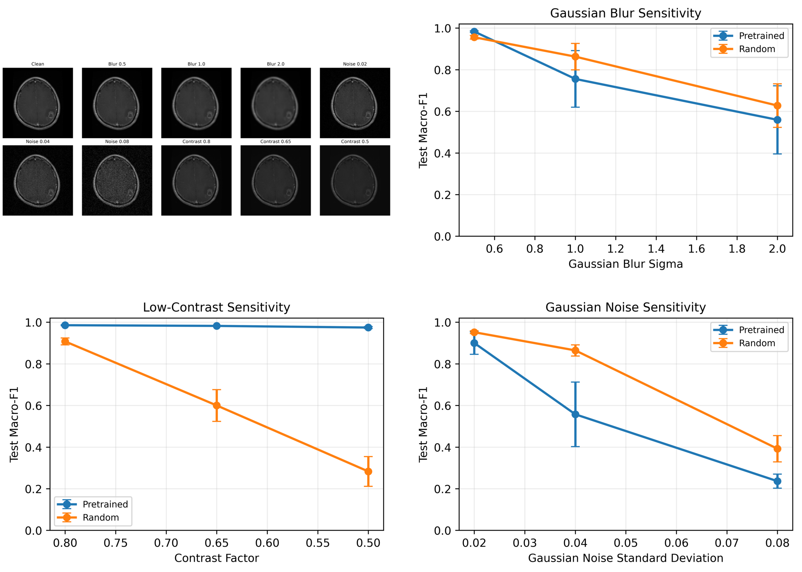
Finally, the test images were changed in controlled ways to examine how model performance responded to lower image quality. Gaussian blur was tested at σ = 0.5, 1.0, and 2.0. Contrast was reduced using factors of 0.8, 0.65, and 0.5. Gaussian noise was added at standard deviations of 0.02, 0.04, and 0.08. These tests measured responses to specific image changes and were not intended to represent real MRI scanner differences.

Evaluation 

Classification performance was measured using accuracy, precision, recall, macro-F1, and ROC-AUC.

Macro-F1 calculates F1 separately for each class and then averages the results, giving each class equal importance:

ROC-AUC measures how well the model separates each class from the others across different prediction thresholds.

Detection was mainly evaluated using mean average precision (mAP), a standard metric for object detection. mAP measures correct tumor classification and how closely the predicted box overlaps the true tumor box.

The overlap between a predicted box and the true box was measured using intersection over union (IoU):

A value of 1 represents perfect overlap between the predicted and true boxes. 

Mean average precision was calculated across tumor classes and IoU thresholds from 0.50 to 0.95:

AP50 and AP75 used overlap requirements of 50% and 75%, respectively.

At a fixed prediction threshold of 0.50, detection precision, recall, missed tumors, and false tumor detections on no-tumor images were also measured. A predicted box counted as correct only if both its tumor class and location matched the true tumor.

Results from seeds 42, 43, and 44 are reported as mean ± standard deviation. Because only three seeds were used, these values describe variation between runs rather than formal statistical significance. Model settings were selected using validation results, not test results.

Ethical considerations

The study used publicly available, de-identified MRI images. No patients were recruited, and no identifiable medical records were accessed.

Because patient identifiers, demographic information, and complete MRI scanning information were unavailable, performance could not be evaluated across individual patients, hospitals, scanners, or demographic groups. The models were developed for research and were not evaluated for clinical decision-making.

Results

Dataset checks

Dataset screening substantially changed the final sample. Among the 5,247 available images, 1,228 groups of exact duplicates were found, including 213 groups that appeared in both the original training and validation folders. Visually similar images were also grouped so related images could not appear in different training, validation, or test sets.

After these checks, 3,710 images remained for classification and 3,573 for detection. No identified duplicate or near-duplicate group appeared in more than one final data split.

Image size was also related to class. In particular, no-tumor images had a different size distribution from the tumor images. A simple model using only image-size information reached about 0.41 accuracy, compared with 0.30 from always predicting the largest class. This suggests that image properties unrelated to the tumor could provide information about the class.

A second public MRI dataset was considered for external testing, but 313 of its 889 test images also appeared in the main dataset. Because the datasets were not independent, it was not used for external testing.

Classification performance

The ImageNet-pretrained ResNet-50 performed better than the same ResNet-50 trained from random weights. Across three seeds, the pretrained model achieved a mean accuracy of 0.9838 and macro-F1 of 0.9855, compared with 0.9611 accuracy and 0.9604 macro-F1 for the random model. The macro-F1 difference was 0.0251.

A third model kept the ImageNet-pretrained ResNet-50 features fixed and trained only the final classification layer. This frozen model achieved a macro-F1 of 0.9262 ± 0.0080, lower than both the fully trained random model and the fully fine-tuned ImageNet model. This indicates that pretrained features were useful, but further training on the MRI images improved performance. Overall classification results are shown in Table 3.

Metric	ImageNet fine-tuning	Random training
Accuracy	0.9838 ± 0.0018	0.9611 ± 0.0063
Macro precision	0.9857 ± 0.0015	0.9636 ± 0.0071
Macro recall	0.9855 ± 0.0016	0.9578 ± 0.0065
Macro-F1	0.9855 ± 0.0016	0.9604 ± 0.0066
Macro ROC-AUC	0.9995 ± 0.0004	0.9967 ± 0.0008

The pretrained model also performed well across all individual classes. Its mean F1 was 0.9821 for glioma, 0.9806 for meningioma, 1.0000 for no tumor, and 0.9794 for pituitary tumor. The random model showed its largest decreases for meningioma and no tumor. Full class-specific precision, recall, and F1 values are provided in Table 4, and the confusion matrices are shown in Figure 2.

Class	Initialization	Precision	Recall	F1
Glioma	ImageNet pretrained	0.9750 ± 0.0104	0.9894 ± 0.0074	0.9821 ± 0.0048
Glioma	Random	0.9683 ± 0.0058	0.9724 ± 0.0133	0.9703 ± 0.0051
Meningioma	ImageNet pretrained	0.9871 ± 0.0063	0.9744 ± 0.0111	0.9806 ± 0.0033
Meningioma	Random	0.9292 ± 0.0144	0.9509 ± 0.0185	0.9398 ± 0.0116
No tumor	ImageNet pretrained	1.0000 ± 0.0000	1.0000 ± 0.0000	1.0000 ± 0.0000
No tumor	Random	0.9806 ± 0.0131	0.9296 ± 0.0170	0.9543 ± 0.0100
Pituitary	ImageNet pretrained	0.9805 ± 0.0062	0.9784 ± 0.0075	0.9794 ± 0.0019
Pituitary	Random	0.9764 ± 0.0129	0.9784 ± 0.0099	0.9773 ± 0.0031

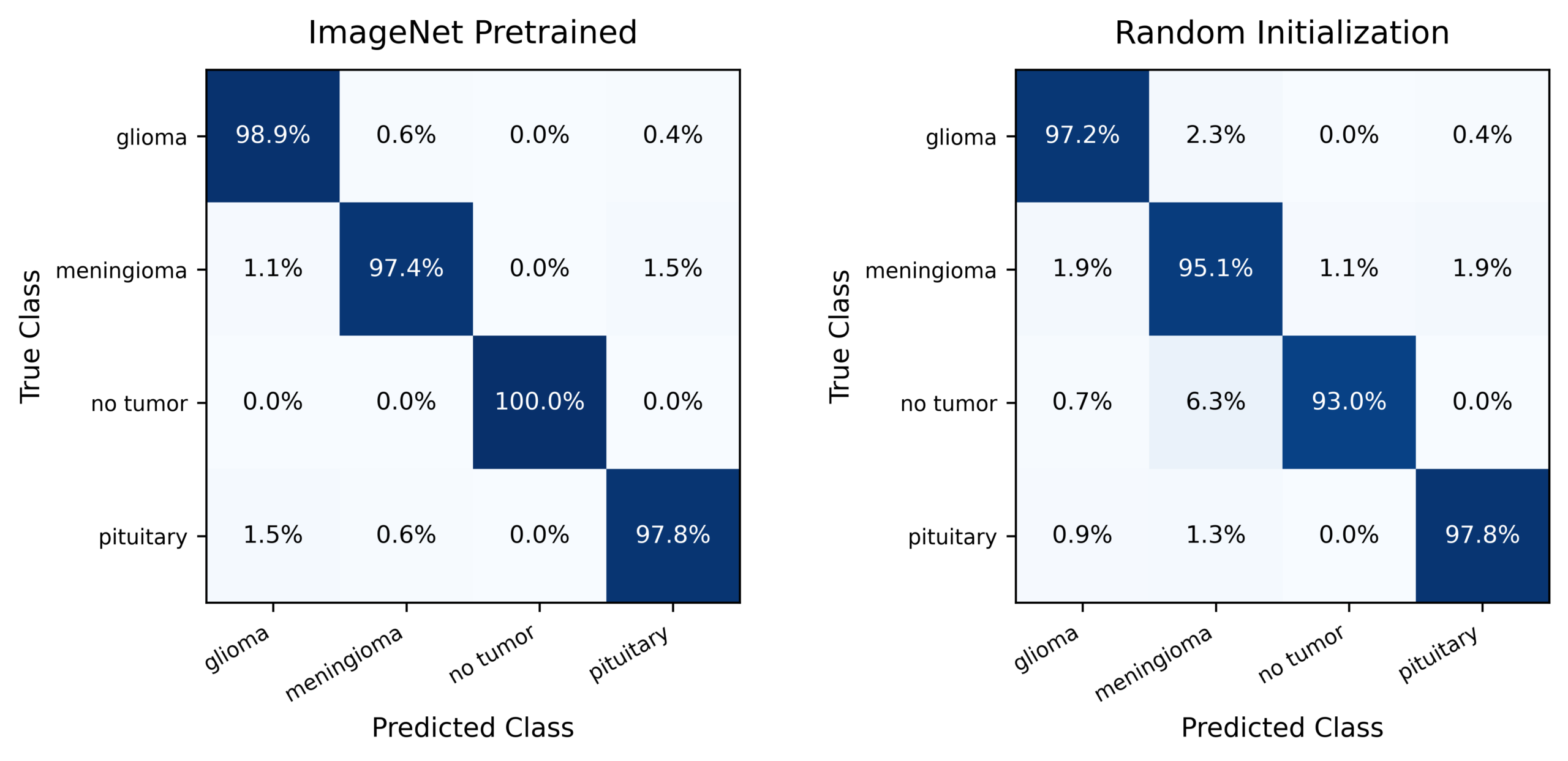
Because the no-tumor images had a different size distribution, classification was also repeated using only the three tumor classes. In this tumor-only analysis, the pretrained model achieved a macro-F1 of 0.9836 ± 0.0054, compared with 0.9628 ± 0.0012 for the random model. The pretrained advantage therefore remained after the no-tumor class was removed, although other image-source differences may still have affected the results.

Training with less data

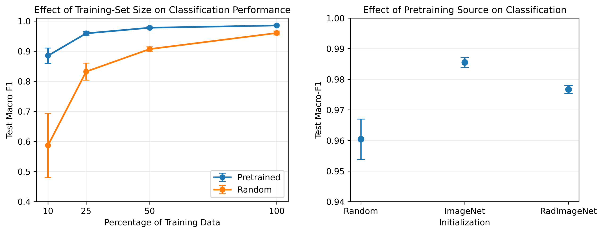
The largest benefit from pretraining appeared when only a small amount of training data was available. With 10% of the training data, the pretrained model achieved a macro-F1 of 0.8851, compared with 0.5872 for the random model. The difference became smaller as more training data were added, reaching 0.9855 versus 0.9604 with the full training set.

The RadImageNet-pretrained model achieved a macro-F1 of 0.9767, higher than random training but slightly lower than ImageNet pretraining in this experiment. Results across training-set sizes and pretraining sources are shown in Table 5, with the trends shown in Figure 3.

Experiment	Condition	Training images	Test macro-F1, mean ± SD
10% training data	ImageNet pretrained	260	0.8851 ± 0.0254
10% training data	Random initialization	260	0.5872 ± 0.1067
25% training data	ImageNet pretrained	650	0.9592 ± 0.0064
25% training data	Random initialization	650	0.8321 ± 0.0281
50% training data	ImageNet pretrained	1,306	0.9779 ± 0.0029
50% training data	Random initialization	1,306	0.9071 ± 0.0072
100% training data	ImageNet pretrained	2,596	0.9855 ± 0.0016
100% training data	Random initialization	2,596	0.9604 ± 0.0066
Pretraining source	RadImageNet pretrained	2,596	0.9767 ± 0.0013

Performance after controlled image changes

Pretraining did not provide better performance under every type of image change. When contrast was reduced, the pretrained model remained relatively stable. At a contrast factor of 0.5, its macro-F1 was 0.9744, compared with 0.2830 for the random model.

The opposite pattern appeared with added noise and stronger blur. At a noise level of 0.04, the pretrained model reached a macro-F1 of 0.5574, while the random model reached 0.8646. Both models performed worse as noise increased.

Full results are provided in Table 6 and Figure 4. These controlled changes do not represent specific MRI scanners or hospitals. They show only that better performance on unchanged test images does not guarantee better performance after every type of image change.

Image Change	Level	ImageNet pretrained	Random
None	0	0.9855 ± 0.0016	0.9604 ± 0.0066
Blur	0.5	0.9833 ± 0.0033	0.9559 ± 0.0087
Blur	1.0	0.7556 ± 0.1360	0.8628 ± 0.0637
Blur	2.0	0.5592 ± 0.1637	0.6276 ± 0.1047
Contrast	0.8	0.9855 ± 0.0028	0.9076 ± 0.0166
Contrast	0.65	0.9822 ± 0.0013	0.6000 ± 0.0762
Contrast	0.5	0.9744 ± 0.0050	0.2830 ± 0.0716
Noise	0.02	0.9000 ± 0.0539	0.9519 ± 0.0066
Noise	0.04	0.5574 ± 0.1552	0.8646 ± 0.0268
Noise	0.08	0.2362 ± 0.0337	0.3921 ± 0.0632

Detection performance

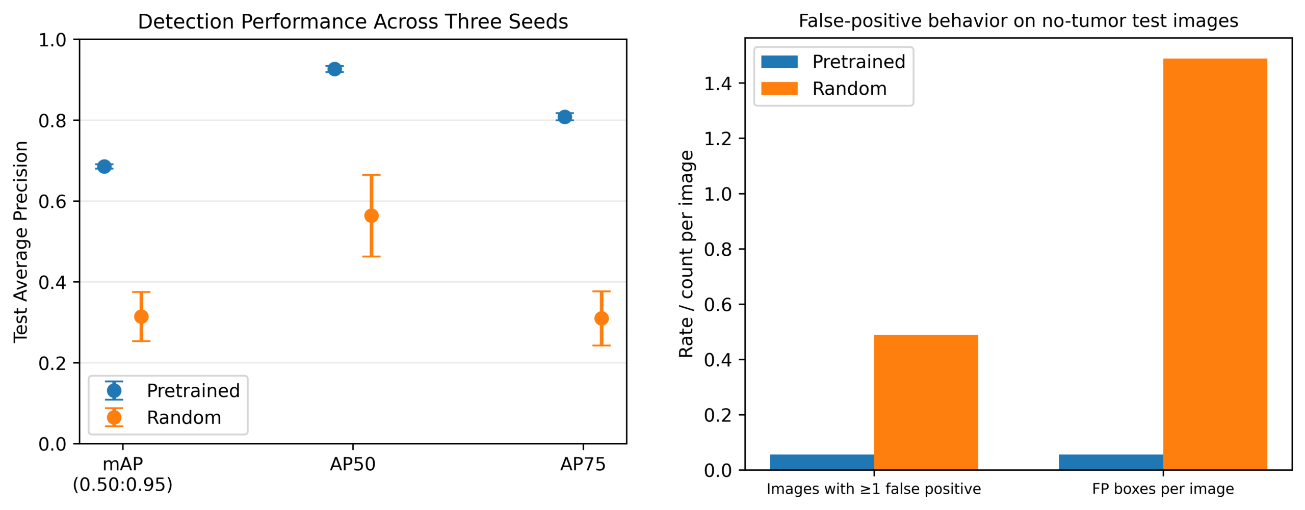
Pretraining produced a much larger difference for tumor detection. Across three seeds, the pretrained Faster R-CNN achieved an mAP of 0.6855 ± 0.0053, compared with 0.3140 ± 0.0609 for the randomly initialized detector.

The pretrained detector also performed better at stricter box-overlap requirements. Its AP50 was 0.9267 and AP75 was 0.8082, compared with 0.5637 and 0.3097 for the random detector. Pretraining also improved performance for all three tumor classes. Detection results across three seeds are shown in Table 7.

Metric	Pretrained	Random
mAP	0.6855 ± 0.0053	0.3140 ± 0.0609
AP50	0.9267 ± 0.0076	0.5637 ± 0.1010
AP75	0.8082 ± 0.0089	0.3097 ± 0.0671
Glioma AP	0.6167 ± 0.0144	0.1231 ± 0.0504
Meningioma AP	0.7760 ± 0.0058	0.4315 ± 0.0810
Pituitary AP	0.6639 ± 0.0077	0.3875 ± 0.0517

At a prediction and box-overlap threshold of 0.50, the seed-42 pretrained detector identified 441 tumors correctly, produced 68 false detections, and missed 39 tumors. Its precision was 0.8664 and recall was 0.9188. The random detector identified 356 tumors correctly, produced 540 false detections, and missed 124 tumors, giving a precision of 0.3973 and recall of 0.7417.

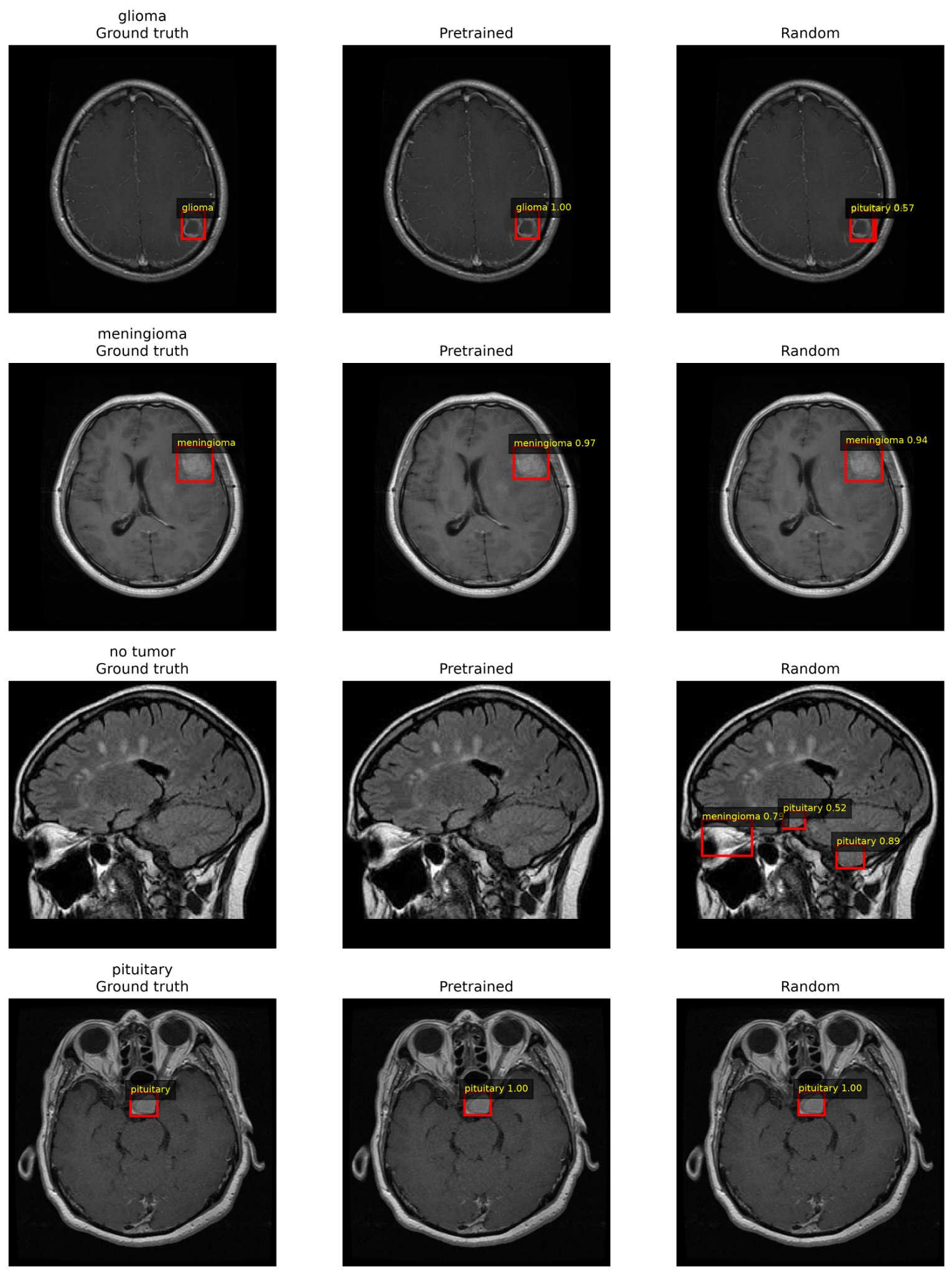
  The difference was also clear on no-tumor images. Among 90 no-tumor test images, the pretrained detector produced at least one false tumor detection on 5 images, or 5.6%, compared with 44 images, or 48.9%, for the random detector. The main detection results are shown in Figure 5, with additional fixed-threshold results in Table 8. Example tumor detections are shown in Figure 6.

Metric	Pretrained	Random
Precision	0.8664	0.3973
Recall	0.9188	0.7417
Missed-detection rate	0.0813	0.2583
Negative images with ≥ 1 false positive	5.6%	48.9%
False positive boxes per no-tumor image	0.056	1.49

Discussion

Main findings

When model structure, data split, and evaluation were kept the same, pretraining improved both brain tumor classification and tumor detection. The classification difference was smaller with the full training set, but the pretrained model still performed better across all three seeds. The detection difference was much larger, with higher mAP, AP50, AP75, recall, and class-specific AP, along with fewer false detections on no-tumor images.

The frozen ImageNet model helps explain the classification result. Its macro-F1 of 0.9262 was lower than both the fully trained random model at 0.9604 and the fully fine-tuned ImageNet model at 0.9855. This suggests that fixed ImageNet features contain useful information, but further training on the MRI images improves performance.

The benefit of pretraining was greatest when fewer training images were available. With 10% of the training data, the macro-F1 difference between the pretrained and random models was about 0.30, compared with about 0.025 using the full training set. This agrees with previous medical-imaging studies showing that transfer learning can be especially helpful when labeled data are limited.^19,20 The value of pretraining therefore appears to depend partly on the amount of task-specific training data available.

Pretraining source and controlled image changes

The RadImageNet results show that medical-image pretraining did not automatically produce the best result. RadImageNet was created from more than one million radiology images and has improved performance in several medical imaging tasks.²² In this study, however, it performed better than random training but slightly worse than ImageNet pretraining.

  This does not mean that ImageNet is generally better than RadImageNet. The models were pretrained on different datasets and used different recommended image-processing settings. The result shows that pretraining source can affect performance and should be tested rather than assumed.

The controlled image changes also showed that higher performance on unchanged test images did not guarantee better performance after every type of image change. The ImageNet-pretrained model remained strong when contrast was reduced but was more affected by added noise and stronger blur. In some of these tests, the randomly initialized model performed better.

These artificial image changes do not show how the models would perform across different MRI scanners, hospitals, or scanning procedures. They only show that performance can depend on the type of image change being tested.

Importance of dataset quality

The dataset checks were an important part of this study. More than 200 exact duplicate groups appeared in both the original training and validation folders. Image size was also related to tumor class, meaning that models could potentially use image properties unrelated to the tumor itself.

A second public MRI dataset could not be used for independent testing because hundreds of its images also appeared in the main dataset. This shows that public medical-image datasets that appear separate may still contain overlapping images.

The final data split prevented identified duplicate and near-duplicate groups from appearing in more than one split. However, reliable patient identifiers were unavailable, so images from the same patient could not be guaranteed to remain together. Complete information about scanners and image sources was also unavailable.

The tumor-only analysis tested if the unusual no-tumor image sizes were responsible for the main classification result. After the no-tumor class was removed, the pretrained model still achieved a higher macro-F1 than the random model. This makes it unlikely that the entire difference was caused by the no-tumor images, although other image-source differences may still exist among the tumor classes.

The results should therefore be interpreted as a comparison of training methods on this dataset, not as evidence of clinical performance.

Detection findings

No-tumor images were treated as images containing no tumor boxes because they do not contain a physical “no tumor” object that should be located.

The pretrained detector also produced far fewer false tumor predictions. Among the 90 no-tumor test images, it produced at least one false detection in 5.6% of images, compared with 48.9% for the random detector. This suggests that pretraining helped the detector avoid incorrectly identifying normal images as containing tumors.

The classification and detection comparisons also used different forms of pretraining. The classifier began with ImageNet weights learned from an image-classification task, while the detector began with COCO-pretrained Faster R-CNN weights learned from an object-detection task. The detection result therefore reflects transfer from both a pretrained image backbone and a pretrained detection system.

Limitations and future work

Several limitations should be considered.

First, the study used a public collection of 2D MRI images without complete patient identifiers, demographic information, scanner information, or scanning settings. The final split prevented known duplicate images from crossing between training and test sets but could not guarantee correct patient-level separation.

Second, the dataset contained different MRI views and image sizes. Complete labels for these differences were unavailable, so performance could not be tested separately for every view or scanner type.

Third, an independent public dataset could not be used for external testing because it shared many images with the main dataset. Testing on a truly independent dataset from another hospital or research group is still needed.

Fourth, the study tested one main model architecture for classification and one for detection, with three random seeds. Other models may respond differently to pretraining.

Fifth, the ImageNet and RadImageNet models used different recommended image-processing settings, so their comparison cannot isolate the effect of the pretraining dataset alone.

Sixth, the blur, contrast, and noise experiments used artificial image changes and do not represent all differences that may occur between real MRI scanners or hospitals.

Finally, the models were not tested in a clinical workflow or compared with physician decisions. Future work should use patient-independent and hospital-independent datasets, include clearer information about image sources, test additional model architectures, and evaluate the models on truly independent clinical data.

Conclusion

When model structure, data split, and evaluation were controlled, pretraining improved brain tumor MRI classification and detection in this public dataset. The classification benefit was largest when less training data were available, while the frozen ImageNet model showed that fixed pretrained features were useful but less effective than full fine-tuning.

Pretraining had an even larger effect on tumor detection, where the pretrained model achieved higher detection performance and produced far fewer false tumor predictions on no-tumor images.

However, duplicate images, class-related image-size differences, and overlap with another public dataset limit how broadly these results can be applied. The findings support pretraining under controlled conditions while also showing the importance of careful dataset checking before drawing strong conclusions about medical AI performance.

References

1. D. N. Louis, A. Perry, P. Wesseling, D. J. Brat, I. A. Cree, D. Figarella-Branger, C. Hawkins, H. K. Ng, S. M. Pfister, G. Reifenberger, R. Soffietti, A. von Deimling, D. W. Ellison. The 2021 WHO classification of tumors of the central nervous system: a summary. Neuro-Oncology. Vol. 23, pg. 1231-1251, 2021, https://doi.org/10.1093/neuonc/noab106. [↩]
2. P. Gao, W. Shan, Y. Guo, Y. Wang, R. Sun, J. Cai, H. Li, W. S. Chan, P. Liu, L. Yi, S. Zhang, W. Li, T. Jiang, K. He, Z. Wu. Development and validation of a deep learning model for brain tumor diagnosis and classification using magnetic resonance imaging. JAMA Network Open. Vol. 5, pg. e2225608, 2022, https://doi.org/10.1001/jamanetworkopen.2022.25608. [↩]
3. A. Akter, N. Nosheen, S. Ahmed, M. Hossain, M. A. Yousuf, M. A. A. Almoyad, K. F. Hasan, M. A. Moni. Robust clinical applicable CNN and U-Net based algorithm for MRI classification and segmentation for brain tumor. Expert Systems with Applications. Vol. 238, pg. 122347, 2024, https://doi.org/10.1016/j.eswa.2023.122347. [↩]
4. Z. N. K. Swati, Q. Zhao, M. Kabir, F. Ali, Z. Ali, S. Ahmed, J. Lu. Brain tumor classification for MR images using transfer learning and fine-tuning. Computerized Medical Imaging and Graphics. Vol. 75, pg. 34-46, 2019, https://doi.org/10.1016/j.compmedimag.2019.05.001. [↩]
5. S. Deepak, P. M. Ameer. Brain tumor classification using deep CNN features via transfer learning. Computers in Biology and Medicine. Vol. 111, pg. 103345, 2019, https://doi.org/10.1016/j.compbiomed.2019.103345. [↩]
6. H. A. Khan, W. Jue, M. Mushtaq, M. U. Mushtaq. Brain tumor classification in MRI image using convolutional neural network. Mathematical Biosciences and Engineering. Vol. 17, pg. 6203-6216, 2020, https://doi.org/10.3934/mbe.2020328. [↩]
7. G. S. Tandel, A. Balestrieri, T. Jujaray, N. N. Khanna, L. Saba, J. S. Suri. Multiclass magnetic resonance imaging brain tumor classification using artificial intelligence paradigm. Computers in Biology and Medicine. Vol. 122, pg. 103804, 2020, https://doi.org/10.1016/j.compbiomed.2020.103804. [↩]
8. J. Kang, Z. Ullah, J. Gwak. MRI-based brain tumor classification using ensemble of deep features and machine learning classifiers. Sensors. Vol. 21, pg. 2222, 2021, https://doi.org/10.3390/s21062222. [↩]
9. R. Hao, K. Namdar, L. Liu, F. Khalvati. A transfer learning-based active learning framework for brain tumor classification. Frontiers in Artificial Intelligence. Vol. 4, pg. 635766, 2021, https://doi.org/10.3389/frai.2021.635766. [↩]
10. A. M. Gab Allah, A. M. Sarhan, N. M. Elshennawy. Classification of brain MRI tumor images based on deep learning PGGAN augmentation. Diagnostics. Vol. 11, pg. 2343, 2021, https://doi.org/10.3390/diagnostics11122343. [↩]
11. C. Srinivas, N. P. K. S. Prasad, M. Zakariah, Y. A. Alothaibi, K. Shaukat, B. Partibane, H. Awal. Deep transfer learning approaches in performance analysis of brain tumor classification using MRI images. Journal of Healthcare Engineering. Vol. 2022, pg. 3264367, 2022, https://doi.org/10.1155/2022/3264367. [↩]
12. M. F. Alanazi, M. U. Ali, S. J. Hussain, A. Zafar, M. Mohatram, M. Irfan, R. AlRuwaili, M. Alruwaili, N. H. Ali, A. M. Albarrak. Brain tumor/mass classification framework using magnetic-resonance-imaging-based isolated and developed transfer deep-learning model. Sensors. Vol. 22, pg. 372, 2022, https://doi.org/10.3390/s22010372. [↩]
13. N. F. Aurna, M. A. Yousuf, K. A. Taher, A. K. M. Azad, M. A. Moni. A classification of MRI brain tumor based on two stage feature level ensemble of deep CNN models. Computers in Biology and Medicine. Vol. 146, pg. 105539, 2022, https://doi.org/10.1016/j.compbiomed.2022.105539. [↩]
14. S. M. Rasa, M. M. Islam, M. A. Talukder, M. A. Uddin, M. Khalid, M. Kazi, M. Z. Kazi. Brain tumor classification using fine-tuned transfer learning models on magnetic resonance imaging (MRI) images. DIGITAL HEALTH. Vol. 10, pg. 20552076241286140, 2024, https://doi.org/10.1177/20552076241286140. [↩]
15. A. Amarnath, A. Al Bataineh, J. A. Hansen. Transfer-learning approach for enhanced brain tumor classification in MRI imaging. BioMedInformatics. Vol. 4, pg. 1745-1756, 2024, https://doi.org/10.3390/biomedinformatics4030095. [↩]
16. R. Disci, F. Gurcan, A. Soylu. Advanced brain tumor classification in MR images using transfer learning and pre-trained deep CNN models. Cancers. Vol. 17, pg. 121, 2025, https://doi.org/10.3390/cancers17010121. [↩]
17. M. A. Khan, M. Z. Hussain, S. Mehmood, M. F. Khan, M. Ahmad, T. Mazhar, T. Shahzad, M. M. Saeed. Transfer learning for accurate brain tumor classification in MRI: a step forward in medical diagnostics. Discover Oncology. Vol. 16, pg. 1040, 2025, https://doi.org/10.1007/s12672-025-02671-4. [↩]
18. S. Rajaraman, G. Zamzmi, F. Yang, Z. Liang, Z. Xue, S. Antani. Uncovering the effects of model initialization on deep model generalization: a study with adult and pediatric chest X-ray images. PLOS Digital Health. Vol. 3, pg. e0000286, 2024, https://doi.org/10.1371/journal.pdig.0000286. [↩]
19. M. Romero, Y. Interian, T. Solberg, G. Valdes. Targeted transfer learning to improve performance in small medical physics datasets. Medical Physics. Vol. 47, pg. 6246-6256, 2020, https://doi.org/10.1002/mp.14507. [↩] [↩]
20. D. Karimi, S. K. Warfield, A. Gholipour. Transfer learning in medical image segmentation: new insights from analysis of the dynamics of model parameters and learned representations. Artificial Intelligence in Medicine. Vol. 116, pg. 102078, 2021, https://doi.org/10.1016/j.artmed.2021.102078. [↩] [↩]
21. R. Zoetmulder, E. Gavves, M. Caan, H. Marquering. Domain- and task-specific transfer learning for medical segmentation tasks. Computer Methods and Programs in Biomedicine. Vol. 214, pg. 106539, 2022, https://doi.org/10.1016/j.cmpb.2021.106539. [↩]
22. X. Mei, Z. Liu, P. M. Robson, B. Marinelli, M. Huang, A. Doshi, A. Jacobi, C. Cao, K. E. Link, T. Yang, Y. Wang, H. Greenspan, T. Deyer, Z. A. Fayad, Y. Yang. RadImageNet: an open radiologic deep learning research dataset for effective transfer learning. Radiology: Artificial Intelligence. Vol. 4, pg. e210315, 2022, https://doi.org/10.1148/ryai.210315. [↩] [↩] [↩]
23. L. Alzubaidi, M. Al-Amidie, A. Al-Asadi, A. J. Humaidi, O. Al-Shamma, M. A. Fadhel, J. Zhang, J. Santamaria, Y. Duan. Novel transfer learning approach for medical imaging with limited labeled data. Cancers. Vol. 13, pg. 1590, 2021, https://doi.org/10.3390/cancers13071590. [↩]
24. Z. Zhou, V. Sodha, J. Pang, M. B. Gotway, J. Liang. Models Genesis. Medical Image Analysis. Vol. 67, pg. 101840, 2021, https://doi.org/10.1016/j.media.2020.101840. [↩]
25. Y. Schirris, E. Gavves, I. Nederlof, H. M. Horlings, J. Teuwen. DeepSMILE: contrastive self-supervised pre-training benefits MSI and HRD classification directly from H&E whole-slide images in colorectal and breast cancer. Medical Image Analysis. Vol. 79, pg. 102464, 2022, https://doi.org/10.1016/j.media.2022.102464. [↩]
26. A. B. Abdusalomov, M. Mukhiddinov, T. K. Whangbo. Brain tumor detection based on deep learning approaches and magnetic resonance imaging. Cancers. Vol. 15, pg. 4172, 2023, https://doi.org/10.3390/cancers15164172. [↩]
27. S. Singh, B. K. Singh, A. Kumar. Magnetic resonance imaging image-based segmentation of brain tumor using the modified transfer learning method. Journal of Medical Physics. Vol. 47, pg. 315-321, 2022, https://doi.org/10.4103/jmp.jmp_52_22. [↩]
28. K. He, X. Zhang, S. Ren, J. Sun. Deep residual learning for image recognition. Proceedings of the IEEE Conference on Computer Vision and Pattern Recognition. Vol. 1, pg. 770-778, 2016, https://doi.org/10.1109/CVPR.2016.90. [↩] [↩]
29. S. Ren, K. He, R. Girshick, J. Sun. Faster R-CNN: towards real-time object detection with region proposal networks. IEEE Transactions on Pattern Analysis and Machine Intelligence. Vol. 39, pg. 1137-1149, 2017, https://doi.org/10.1109/TPAMI.2016.2577031. [↩] [↩]
30. T.-Y. Lin, P. Dollar, R. Girshick, K. He, B. Hariharan, S. Belongie. Feature pyramid networks for object detection. Proceedings of the IEEE Conference on Computer Vision and Pattern Recognition. Vol. 1, pg. 2117-2125, 2017, https://doi.org/10.1109/CVPR.2017.106. [↩] [↩]
31. J. Deng, W. Dong, R. Socher, L.-J. Li, K. Li, L. Fei-Fei. ImageNet: a large-scale hierarchical image database. Proceedings of the IEEE Conference on Computer Vision and Pattern Recognition. Vol. 1, pg. 248-255, 2009, https://doi.org/10.1109/CVPR.2009.5206848. [↩]
32. A. Sorour. MRI for brain tumor with bounding boxes. Kaggle, https://www.kaggle.com/datasets/ahmedsorour1/mri-for-brain-tumor-with-bounding-boxes, 2021. [↩]
33. T.-Y. Lin, M. Maire, S. Belongie, J. Hays, P. Perona, D. Ramanan, P. Dollar, C. L. Zitnick. Microsoft COCO: common objects in context. European Conference on Computer Vision. Vol. 8693, pg. 740-755, 2014, https://doi.org/10.1007/978-3-319-10602-1_48. [↩]