Abstract
Classical aerodynamic theory predicts that power scales with the cube of velocity when air density, drag coefficient, and reference area remain approximately constant. However, cross-category comparison is limited by non-standardized power and velocity specifications reported under different operating regimes. In this work, we examine the relationship between power and velocity using data. The data is collected from commercially deployed aeroplanes, unmanned aerial vehicles (UAVs), and battery-powered drones. Seventy-six aircrafts’ power and velocity data were collected from manufacturer specifications. Where the data was unavailable, it was derived using standard mechanical relations. The formulas are mentioned in the datasheets of the aircrafts. This method used other quantities available in the manufacturers’ datasheet. By analysing log-log plots of power versus velocity, we observe linear trends with slopes ~3 across all categories, consistent with theoretical expectations. All the three aircrafts’ dataset showed moderately strong to strong, based on the scale mentioned, linear associations. The greater scattering of datapoint among aircrafts may reflect differences in configuration, power definitions, payload, and test conditions, although these effects could not be independently quantified. Deviations from the ideal cubic exponent are discussed in terms of aerodynamic efficiency, altitude-dependent air density, and vehicle geometry. This study provides an exploratory analysis of publicly available specification data. It does not constitute controlled experimental verification of the cubic power-velocity law, across several orders of magnitude in mass and speed, highlighting its relevance to aircraft design, propulsion optimisation, and engineering education.
Introduction
Evolution of vehicles over a period
The evolution of vehicles has been one of humanity’s historic accomplishments. From the earliest days, humans relied on walking. Following the technological breakthrough of the invention of the wheel, humans began to travel in carts and chariots. Around 4000 BCE, boats and sailing ships were developed, powered by wind for sea travel. The revolution in vehicles took place with the independence of animals from road transportation, also with the utilization of wind power for sailing, following the invention of steam engine in 1698 by Thomas Savery.1 In 1712, Englishman, Thomas Newcomen, developing a more efficient steam engine with a piston separating the condensing steam from the water. In 1765 James Watt greatly improved the Newcomen engine by adding a separate condenser to avoid heating and cooling the cylinder with each stroke.1 Watt then developed a new engine that rotated a shaft instead of providing the simple up-and-down motion of the pump, and he added many other improvements to produce a practical power plant. This revolution made all means of transportation, including railways, use the same engine for greater efficiency. During World War I (1914–1918), military aviation developed rapidly. Aircraft capabilities improved significantly. Aerial tactics also advanced. Aerial photography became more developed. Aircraft weaponry also improved during the war.2 Later in the 20th and 21st centuries, the use of hybrid engines, which operate on power from both combustion engines and batteries, increased due to environmental concerns, as combustion engines emit nitrogen, hydrocarbon, etc. gases, resulting in pollution and environmental degradation.3 Power, velocity and mass significance Velocity plays a significant role in the working of aerial vehicles. It is a major measured quantity which helps quantify the output of the vehicle. We can calculate various derived quantities like lift, stall velocity, and kinetic energy as discussed below.
Flight velocity is a central variable in aircraft performance because aerodynamic drag varies with velocity and the power required to overcome drag is the product of drag force and flight velocity. Power is the work done in a unit of time. Displacement is required to define the work done. Since movement is the fundamental principal of transportation, and the development of vehicles fulfils that need, thus displacement is defined. Hence, work will be done in some time. Combining work and displacement, we get power. Also, aircraft generate thrust and move with a certain velocity simultaneously, which leads us to the relationship of the power consumption, which says P = F.V, F and V are the force and velocity.
Thus, to maintain velocity at a given thrust, power is required. Mass also plays an important to quantify thrust as it should be more the weight  of the aircraft to make the aircraft fly.
Importance of aerial vehicles
Aerial vehicles are systems that work on the principle of lift and propulsion. They are designed to be operated in an atmosphere. The breakthrough of the aerial vehicle played a significant role in development. It influences areas of development, such as transportation, defence, and science. Aerial vehicles have various advantages that set them apart from other types of vehicles. They offer high-speed service and long-distance transportation with minimal geographic limitations. Commercial aircraft facilitate the global movement of passengers and goods. These advantages offered by aerial vehicles support international trade and economic integration. In logistics, air transport is crucial for time-sensitive and high-value shipments. The defence and security sector is highly dependent on aerial vehicles. Reconnaissance, intelligence gathering, and other strategic operations require aerial vehicles such as fighter jets and surveillance aircraft. Aerial vehicles also facilitate scientific and environmental research. These vehicles are specialized to support weather observation and remote sensing. In agriculture, these vehicles are commonly used for infrastructure management, including spraying and seeding. used such vehicles are used for mapping and structural inspection. Hence, drones serve as tools for development in modern society.
Types of UAV
UAV are broadly defined under three categories i.e. fixed wing, rotary wing, Hybrid/VTOL.4 Fixed wing drone generate lift using their rigid aerodynamically designed wings. They require forward motion to stay airborne. Because of their aerodynamics, they require less power to remain airborne, increasing their endurance. These drones are less stable than multirotor drones and cannot hover in one place. rotary wings comprise of broadly two categories i.e. single rotor and multi rotor.4 Multi-rotor drones use multiple rotors to generate lift and control motion. They work on the principle of upthrust, in which they exert more upthrust than their own weight. They are capable of taking off, hovering, and landing vertically. They offer high stability, but they consume power at a high rate, resulting in limited endurance. Single-rotor drones use a single main rotor to generate lift and a torque-compensating mechanism at the tail to improve stability. They exhibit low disk loading, enabling higher payload capacity. They generate more lift than multirotor mechanisms. They are mechanically complex and require higher maintenance. Hybrid VTOL (Vertical Take-Off and Landing) drones have both a multirotor mechanism and good aerodynamics, like multirotor and fixed-wing drones; they can take off and land vertically and remain airborne using their fixed wings. It is capable of hovering and long-range operations. It is more energy efficient than multirotor drones during forward flight. It is suitable for confined take-off areas with long missions. These are very complex and, because of these features, are generally used in warfare.
Aircraft power sources
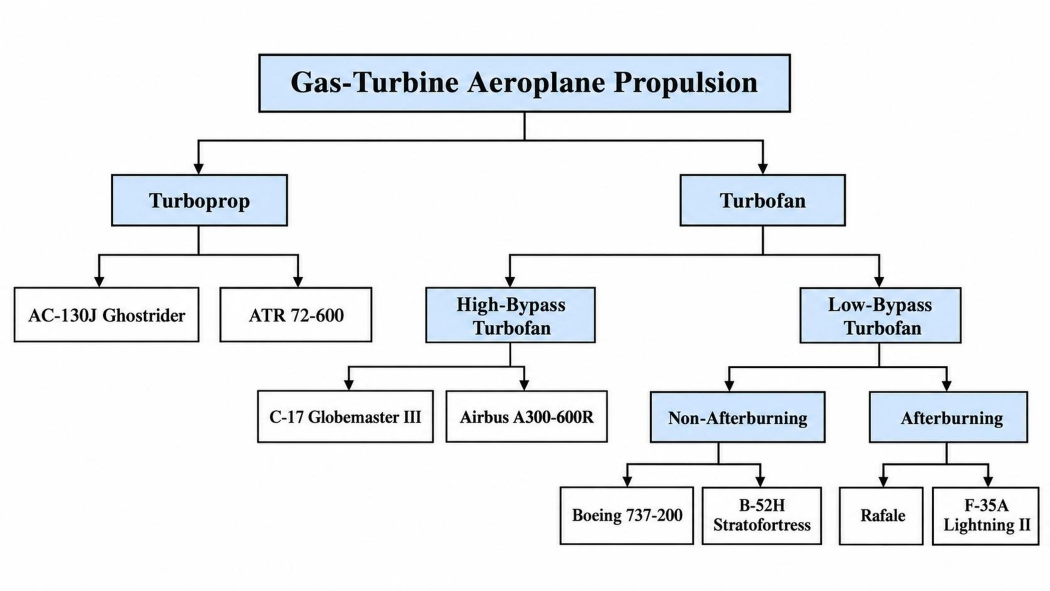
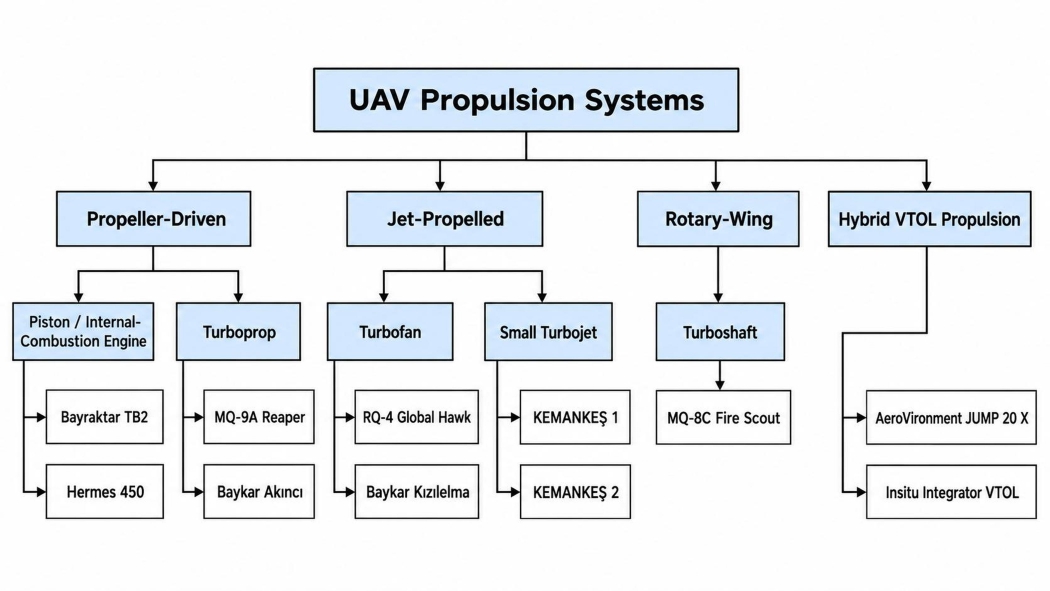
The engine of a drone is a vital component. It primarily determines flight performance, payload capacity, endurance, and operational flexibility. The following flowcharts explain each type of engine under all three categories: Aeroplane, UAV, Battery drones, along with two examples of each category from the datasheet mentioned under “Data and Statistical Analysis”
Aeroplane Power Sources
UAV Power Sources
Battery Drones
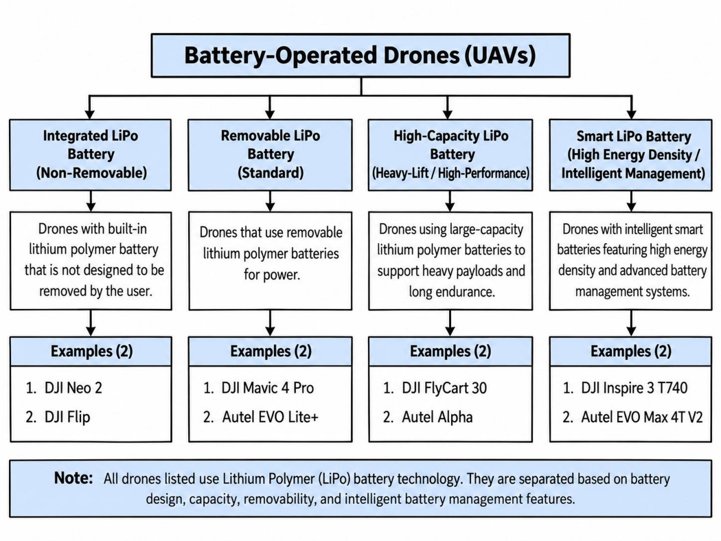
Terminology
Rotary-wing aircraft generate lift using spinning wing-shaped rotors. Hybrid fixed/rotary-wing aircraft, also called compound rotorcraft, combine rotors with propellers, thrust engines, or fixed lifting surfaces. Piston engines use reciprocating pistons to convert pressure into rotating motion. Turboprop engines use a turbine to drive both the compressor and the propeller. Turboshaft engines produce shaft power to drive helicopter rotors instead of direct jet thrust.5 Turbojets are the simplest aircraft gas turbine engines. Turbofan engines split airflow between the core and bypass duct to produce thrust efficiently. Low-bypass turbofans are suited to high-speed military aircraft. High-bypass turbofans produce most thrust from bypass air and are suited to subsonic transport aircraft. Afterburners are secondary combustion chambers used to increase thrust in military aircraft.5
Literature review
Aircraft power-velocity scaling is not a single-regime phenomenon. It emerges from the changing balance among parasite drag, induced losses, rotor profile losses, propulsion efficiency, and mission constraints. Zeng and Zhang6 provided a widely used fixed-wing propulsion formulation in which the parasite-power contribution rises with the cube of airspeed, whereas the induced-power contribution decreases as speed increases. Their analysis therefore supports a cubic dependence only in the parasite-drag-dominated portion of the flight envelope, not as a universal relation from low-speed flight to maximum speed. For rotary-wing aircraft, Zeng et al.7 derived a structurally different power model containing blade-profile, induced, hover, and parasite terms. That formulation predicts a non-monotonic power curve and separates the speeds that maximize endurance from those that maximize range. At the delivery-system scale, Stolaroff et al.8 showed that vehicle size, payload, battery requirements, and logistics architecture can materially alter energy use and environmental performance. Taken together, these foundational studies establish the principal theoretical constraint on cross-platform scaling: a near-cubic exponent is physically interpretable only when the aerodynamic and propulsive quantities embedded in the proportionality constant remain sufficiently stable. A second strand of the literature has improved the empirical basis of aircraft energy analysis by linking propulsion theory to direct measurement. Zhao et al.9 developed an airborne electric-propulsion measurement system for fixed-wing UAVs and demonstrated the simultaneous acquisition of motor speed, voltage, current, thrust, torque, efficiency, and airspeed in wind-tunnel and outdoor flight tests. Rodrigues et al.10 subsequently created a high-resolution dataset from 209 autonomous quadcopter flights in which commanded speed, cruise altitude, payload, wind, voltage, current, position, orientation, velocity, and acceleration were recorded under repeated operating conditions. This dataset is especially important methodologically because it distinguishes measured power under matched conditions from isolated manufacturer specifications. Broader vehicle-energy analyses reinforce the same point. Zhang et al.11 showed that the energy balance of solar-powered UAVs is coupled to irradiance, incidence angle, attitude, and power-system parameters, while Aiello et al.12 embedded aircraft dynamics and environmental constraints within energy-efficient three-dimensional path planning. These contributions move the literature away from speed-only explanations and toward condition-specific power models in which propulsion, environment, and trajectory are treated as interacting variables.
For multicopters, the strongest evidence against a universal speed law comes from studies of optimal cruise, mission phase, and configuration. Bauersfeld and Scaramuzza13 combined aerodynamic, motor, and battery models with experimental validation to estimate multicopter range, endurance, and optimal speed. Their results show that neither minimum nor maximum speed is generally optimal; range and endurance peak at different intermediate speeds because aerodynamic demand and electrical losses vary differently across the flight envelope. Using field data from delivery missions, Rodrigues et al.14 further demonstrated that energy use must be interpreted across take-off, cruise, and landing rather than reduced to a single cruise-speed value. Configuration changes can alter the governing balance even more fundamentally. Zhang et al.15 showed that lifting-wing multicopters can transfer part of the lift burden from the rotors to aerodynamic surfaces, thereby changing rotor loading, cruise power, and range. Carreño Ruiz et al.16, using experiments and computational-fluid-dynamics analysis, demonstrated that small rotors operating at low Reynolds numbers exhibit performance characteristics that simplified high-Reynolds-number assumptions do not capture reliably. Collectively, these studies indicate that vehicle geometry and flow regime can change both the magnitude and the shape of the power-speed relation.
The modelling literature has therefore expanded beyond classical closed-form expressions. Góra et al.17 used machine learning to construct a UAV energy-consumption model from measured operational variables, illustrating how data-driven methods can represent relationships that are difficult to encode through geometry-dependent equations alone. In agricultural rotorcraft, Zhu et al.18 identified statistically significant associations between energy use and operational variables including forward speed, acceleration, and repeated turning manoeuvres. Dai et al.19 generalized rotary-wing propulsion modelling by incorporating thrust-to-weight ratio, acceleration, and changes in flight direction, while Gong et al.20 derived and validated power-consumption expressions for both forward and three-dimensional multirotor flight. Platform specificity remains evident even within the rotary-wing class: Żugaj et al.21 found that unmanned-helicopter energy demand depends on rotor speed, manoeuvre type, and control settings. Głębocki et al.22 then used Monte Carlo simulation to show that uncertainty in model parameters propagates into non-negligible uncertainty in predicted mission energy. The cumulative implication is important for scaling analysis: an observed regression exponent may summarize a dataset effectively while still concealing substantial variation in the mechanisms that generate power demand.
Environmental exposure and mission architecture introduce additional departures from nominal performance. Han et al.23 conducted a flight-testing campaign under atmospheric icing and found that ice accretion reduced lift, increased drag, obstructed Pitot-probe measurements, degraded propeller performance, and required more than 80% additional power to complete the same mission. This result demonstrates that even the same aircraft on the same trajectory can occupy a markedly different power regime when its aerodynamic surfaces or propulsion system are altered by the environment. At the mission level, Van Mulders et al.24 showed that the energy and ecological consequences of UAV-based servicing depend on hover duration, service distance, payload, and the system being replaced. Mohiuddin et al.25 demonstrated that cooperative payload transportation by two UAVs can be improved through optimized velocity profiles rather than operation at a fixed or maximum speed. These studies reinforce a consistent conclusion across the literature: power is a property of an aircraft-state-environment-mission combination, not of speed in isolation. Recent data-driven work has sought greater accuracy and transferability without requiring complete aerodynamic descriptions. Dai et al.26 developed a stacking ensemble from flight records of three quadrotor types and showed that a compact feature set comprising aircraft mass, kinematic state, and wind can support accurate, data-efficient power estimation across platforms. Çabuk et al.27 compared theoretical, polynomial, and machine-learning models for small-drone swarm missions and identified an energy-efficient airspeed region rather than a universal optimum. Using data from 279 flights, Ait Saadi et al.28 evaluated 23 recurrent-neural-network variants and found that bidirectional long short-term memory models best captured the temporal structure of UAV power consumption. Abd El-Latif and El-dosuky29 combined optimized mathematical models, random-forest regression, and explainable-AI analysis to examine the contributions of mass, payload, thrust, airspeed, altitude, and environmental conditions. Kim et al.30 addressed the weakness of velocity-only neural models by introducing a hybrid framework that estimates otherwise unavailable vibration-acceleration effects; their experimentally evaluated model achieved a root-mean-squared percentage error of 6.12% and improved substantially over a DNN-only baseline. At the whole-aircraft level, Li et al.31 coupled mass, motor efficiency, and electrochemical-aging-thermal battery dynamics in a multidisciplinary eVTOL optimization framework, reporting an 11.44% reduction in total energy consumption relative to the baseline design. These results show that improved predictive performance generally comes from adding state, environment, configuration, or temporal information rather than from refining a velocity-only law. Two recent fixed-wing studies further clarify the physical connection between propulsion state and speed while also exposing the limits of specification-based inference. Ntouros et al.32 derived an analytical airspeed estimator based only on propeller power and rotational-speed feedback, calibrated it using blade-element-momentum simulations, wind-tunnel data, and flight tests, and achieved approximately 5% normalized root-mean-square error on unseen flight data. The study provides direct evidence that propulsion measurements contain recoverable information about airspeed, but the relationship is platform-calibrated rather than universally transferable. Bauer33 approached the same coupling from the control perspective, validating a modified total-energy-control scheme in simulation and real flight tests; the controller coordinated indicated airspeed, altitude, elevator, and throttle while maintaining stall protection. Together, these works confirm that power and speed are dynamically coupled in flight, yet they also show that the coupling is mediated by aircraft-specific propulsion, aerodynamics, control logic, and operating state.
The literature therefore converges on three conclusions. First, cubic power scaling has a sound aerodynamic basis for fixed-wing parasite-drag-dominated flight. Second, rotary-wing, hybrid-lift, and mission-level systems contain additional power terms that can dominate outside that regime. Third, the most accurate contemporary models require variables beyond speed, including mass, acceleration, attitude, wind, altitude, rotor state, battery behaviour, and mission phase7,10. What remains comparatively underexamined is a different, deliberately cross-sectional question: whether publicly reported nominal power and maximum-speed specifications for commercial aeroplanes, engine-driven UAVs, and battery drones display an emergent category-level scaling trend across several orders of magnitude. Existing studies usually analyse matched measurements from one platform, one vehicle family, or one defined mission; they do not test the statistical structure of heterogeneous specification data across fundamentally different aircraft classes.
The present study addresses that gap through exploratory log-log regression within three vehicle categories. Its objective is not to claim that maximum power and maximum velocity were measured simultaneously, nor to treat a fitted exponent as direct experimental verification of a universal aerodynamic mechanism. Manufacturer-reported power may denote rated, continuous, take-off, shaft, electrical-input, or system power, while reported maximum velocity may depend on altitude, payload, configuration, atmospheric conditions, and test procedure. These inconsistencies limit direct comparability and are treated as sources of structural uncertainty rather than random measurement noise. Within those constraints, the analysis asks whether a near-cubic trend remains visible at the category level and whether the fitted exponents differ systematically among commercial aeroplanes, engine-driven UAVs, and battery drones. Framed in this way, the study complements not replaces the controlled theoretical and experimental literature: it evaluates the large-scale empirical pattern present in public specifications while explicitly separating statistical scaling from causal aerodynamic validation.
Methodology
Data acquisition method
Data collection involves systematically gathering information for analysis. To examine the relationship between velocity and power in aerial vehicles, data on power (kW), velocity (km/hr), and mass (kg) are necessary, since mass also significantly influences this relationship. Data had been collected based on the availability under the following priority order mentioned: Priority 1: Official manufacturer data Priority 2: Government or institutional sources Priority 3: Technical databases & research papers / Quantification Using Standard Formulae
NOTE: The sources and the websites of the specifications are mentioned in datasheet.
Analytical Derivation of the Power-Velocity Scaling Law
For an aerial vehicle moving at a constant airspeed  , the aerodynamic parasite drag is given by the standard drag equation
where  is the parasite drag force,
 is the air density,
 is the drag coefficient,
 is the aerodynamic reference area, and is the airspeed relative to the surrounding air.34
The reference area represents the characteristic projected area used to define the aerodynamic drag coefficient. For parasite drag, it commonly corresponds to the frontal area exposed to the airflow.
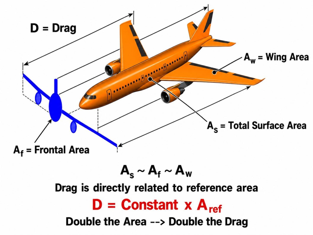
During steady, level flight at constant airspeed, thrust acts in the direction of motion, while drag acts in the opposite direction. Because the streamwise acceleration is zero, the magnitudes of thrust and drag are equal.35 The mechanical power required to maintain the airspeed is the product of the force opposing motion and the velocity:
Substituting the drag equation from equation1 into the power expression gives  Therefore,
 .
Provided that , , and remain approximately constant over the investigated velocity range,  constant. Hence,
This cubic relationship applies specifically to the power required to overcome parasite drag. It is valid primarily in the parasite-drag-dominated regime and should not be interpreted as a universal relationship for total propulsion power over the entire flight envelope. At low airspeeds, induced power may form a substantial or dominant part of the total power requirement.
Logarithmic transformation of the Cubic Power-Velocity Relationship
Let
Then the cubic relationship can be written as  , Taking the base-10 logarithm of both sides gives

Using the logarithmic identities
Equation becomes  . Substituting the expression for
 ,
Equation 5 has the linear form  ,
Where  ,
 ,
 , and
 .
Therefore, an ideal log-log plot of parasite-drag power against velocity should produce a straight line with a theoretical slope of For empirical data, the relationship may be written more generally as
where  is the experimentally determined power-law exponent, and
 represents residual variation caused by differences in aircraft configuration, operating conditions, propulsion efficiency, and omitted power components. The theoretical cubic law predicts
 . Thus, the fitted value of can be compared with 3 to evaluate how closely the observed power–velocity relationship follows the parasite-drag scaling law.
Power’s uncertainty calculation
For gas-turbine-powered aircraft, a conservative cycle-model precision uncertainty of  was adopted. This value corresponds to the larger of the combined physics-modelling and numerical uncertainties reported for gas-turbine shaft power, namely
 for the high-pressure spool and for the low-pressure spool.36 This uncertainty represents only the precision of gas-turbine cycle modelling and does not include differences in aircraft configuration, operating conditions, measurement procedures, or omitted aerodynamic power components.36.
The power uncertainty is therefore
The corresponding power interval is
For the logarithmic regression model, log10 Ppredicted = C + blog10 V + ε,
Where  from equation 5is the theoretical intercept and is the power-law exponent. The logarithmic uncertainty is calculated using
Substituting  ,
 ,
And  . Therefore, the approximate base-10 logarithmic uncertainty is
 , or approximately,
 .
Significance of this Relation in Engineering
The relationship between power and velocity plays a significant role, as it is widely used in many fields of engineering, especially mechanical engineering, where it is often used to determine the power required to achieve a given speed.
Here are the fields of engineering where this relationship is used the most,
Renewable Energy Engineering
The relation between the power and the velocity is the fundamental basis of the extraction of power from wind and its conversion into energy. The power generation is solely dependent on the speed of the wind, so even a trivial amount of increase in velocity would give a very high-power output. Wind power is proportional to wind speed cubed.
Civil Engineering
The relation indirectly defines the infrastructure with respect to the geographical conditions. Safe heights of the tower are defined. Civil engineers use this relation to estimate the energy of the wind and thus the force exerted by the wind at a certain height, and hence engineers design aerodynamically sustainable structures of skyscrapers.
Mechanical Engineering
The core application of this relationship in mechanical engineering is the designing of the fans and blowers used to move air through ducts. These are generally used to make heat blowers, exhaust cooling systems, and for generating a vacuum. The factor that determines the amount of power consumption is rotational speed and motor power. This is one of the reasons behind the increase in the cost of the electricity bill when fans and coolers are used at their maximum speed.
Industrial Engineering
Factories’ temperature rises due to extensive use of machinery, which converts power to heat. To counter that, factories often require ventilation involves flow of air. These units work on the principle of propulsion. To get the maximum cooling with cost efficiency, the factories prefer using larger propellers or bigger fans instead of smaller propellers with higher RPM, as the power shows the relation with the cube of velocity to be directly proportional.
Hence, the cubic relationship between power and velocity is used frequently in engineering, depending on the application. It is used to maintain a balance between velocity and the power supplied or generated, resulting in a sustainable and economically feasible outcome.
Data Analysis Approach
The relationship between power and velocity was analysed using a log-log graphical approach. The power and velocity values for each aerial vehicle were first converted into their logarithmic forms. The logarithm of power was then plotted against the logarithm of velocity on a Cartesian coordinate plane.A linear regression line was fitted to the plotted data, and its slope was calculated. Since a power-law relationship of the form P ∝ vⁿ becomes linear after logarithmic transformation, the slope of the regression line represents the exponent n. The calculated slope was therefore compared with the theoretical value of 3 expected from the cubic power-velocity relationship. Correlation coefficients and the distribution of data points around the regression line were also examined to evaluate the strength and consistency of the observed relationship. Errors and uncertainties arising from published specifications, unit conversions, calculated power values, and differences in operating conditions were considered before drawing the final conclusions.
Additional limitations, including variations in aircraft mass, altitude, propulsion system, aerodynamic configuration, payload, and data-source reliability, were also taken into account while interpreting the results.
Basic Features of the Graphs
A linear scale has been used for plotting data points. Logarithms were used to show the relationship P ∝ v³ as a linear relationship and to compress wide ranging power and velocity to a smaller scale to study. Max gross take-off weight in kg is just for reference for the sake of physical interpretability but is not plotted on the graph. To preserve the individuality and originality of the data of each aerial vehicle, a scatter plot was chosen. A linear trend line is chosen to represent the whole dataset linearly, which also represents the behaviour and the trajectory of the graphs.
Axes used for plotting graphs (common to all three graphs)
X-axis: log₁₀(velocity)
Each data point represents the velocity of a real, physically existing aerial vehicle or aircraft, not an averaged or idealized model. The following axis represents the maximum velocity in km/hr that could be attained by the aircraft relative to the air.
Y-axis: log₁₀(power)
Each data point represents the power used by a real, physically existing aerial vehicle or aircraft, not an averaged or idealized model. The following axis represents the power in kW that is required by an aerial vehicle to be operated at its maximum velocity.
Data and Statistical Analysis
Methodological Notes
NOTE: For all three datasets, the highest reported power, speed, and take off-weight values were used where multiple values were available. Power was obtained from published ratings or estimated using the applicable method, including  , shaft-power conversion, or
 , selected as a representative altitude within the aircraft’s operational limits. MTOW or MGTOW was used only when explicitly stated by the manufacturer; otherwise, the published take-off mass was retained.
LIMITATIONS: The most accurate and reliable publicly available specification data were collected; however, the vehicles were not tested under identical conditions, and fully matched power and velocity data at the same altitude, payload, configuration, and operating state were not practically accessible. Reported power and maximum speed were often obtained under different conditions and were not measured simultaneously. Rated thrust, shaft power, average battery power, mechanical propulsive power, and maximum motor power are not directly equivalent. Differences in altitude, payload, wind, temperature, battery condition, propulsion efficiency, configuration, and test procedure introduce additional uncertainty. Therefore, the datasets support a comparative empirical investigation of the  – relationship but do not constitute strict experimental proof of
 .
Datasheets
Aeroplane
| Aircraft | Power (kW) | Speed (km/h) | MGTOW (kg) | log10 (Vel.) | log10 (Power) | Formula |
| AC-130J Ghostrider | 13,827 | 669 | 74,389 | 2.825 | 4.141 | NA |
| AC-130W Stinger II | 12,822 | 556 | 70,306 | 2.745 | 4.108 | NA |
| C-32 | 70,841 | 853 | 115,666 | 2.931 | 4.850 | P = TV |
| Boeing 737-200 | 23,327 | 870 | 52,390 | 2.940 | 4.368 | P = TV |
| Rafale | 56,756 | 1,389 | 24,493 | 3.143 | 4.754 | P = TV |
| C-17 Globemaster III | 181,083 | 906 | 265,352 | 2.957 | 5.258 | P = TV |
| C-130E Hercules | 12,527 | 555 | 69,750 | 2.744 | 4.098 | NA |
| C-130H Hercules | 13,694 | 589 | 69,750 | 2.770 | 4.137 | NA |
| C-130J Hercules | 14,018 | 671 | 74,393 | 2.827 | 4.147 | NA |
| B-52H Stratofortress | 175,790 | 1,046 | 219,600 | 3.020 | 5.245 | P = TV |
| A-10C Thunderbolt II | 30,598 | 676 | 22,950 | 2.830 | 4.486 | P = TV |
| Embraer E175 | 31,210 | 871 | 38,790 | 2.940 | 4.494 | P = TV |
| ATR 72-600 | 4,101 | 500 | 23,000 | 2.699 | 3.613 | NA |
| Cessna Citation CJ4 | 9,796 | 1,094 | 7,761 | 3.039 | 3.991 | P = TV |
| T-6A Texan II | 820 | 515 | 2,955 | 2.712 | 2.914 | NA |
| HondaJet Elite II | 18,238 | 782 | 5,669 | 2.893 | 4.261 | P = TV |
| P-8A Poseidon | 60,518 | 907 | 85,820 | 2.958 | 4.782 | P = TV |
| Pilatus PC-24 | 27,680 | 814 | 8,500 | 2.911 | 4.442 | P = TV |
| Gulfstream G280 | 19,425 | 1,048 | 17,962 | 3.020 | 4.288 | P = TV |
| Gulfstream G800 | 51,658 | 1,145 | 47,899 | 3.059 | 4.713 | P = TV |
| Gulfstream G700 | 47,309 | 1,049 | 48,806 | 3.021 | 4.675 | P = TV |
| Gulfstream G600 | 44,171 | 1,133 | 42,910 | 3.054 | 4.645 | P = TV |
| Gulfstream G500 | 42,663 | 1,133 | 36,106 | 3.054 | 4.630 | P = TV |
| Bombardier Global 6000 | 35,753 | 933 | 45,132 | 2.970 | 4.553 | P = TV |
| Cessna Citation Mustang | 2,177 | 629 | 3,921 | 2.799 | 3.338 | NA |
| Cessna Citation Longitude | 16,955 | 895 | 17,916 | 2.952 | 4.229 | P = TV |
| Cessna Citation Latitude | 12,057 | 826 | 13,971 | 2.917 | 4.081 | P = TV |
| Cessna Citation Sovereign | 8,948 | 850 | 13,743 | 2.929 | 3.952 | NA |
| Praetor 600 | 16,055 | 863 | 19,440 | 2.936 | 4.206 | P = TV |
| Cirrus Vision SF50 | 2,684 | 587 | 2,721 | 2.769 | 3.429 | P = TV |
| F/A-18F Super Hornet | 105,579 | 1,960 | 29,900 | 3.292 | 5.024 | P = TV |
| Bombardier Challenger 650 | 23,723 | 1,041 | 17,236 | 3.017 | 4.375 | P = TV |
| HondaJet HA-420 | 3,862 | 781 | 4,808 | 2.893 | 3.587 | P = TV |
| Aerospatiale SN-601 Corvette | 4,695 | 760 | 6,600 | 2.881 | 3.672 | P = TV |
| Airbus A300-600R | 58,693 | 897 | 170,500 | 2.953 | 4.769 | P = TV |
| BAE Systems Avro RJX100 | 30,935 | 894 | 25,450 | 2.951 | 4.490 | P = TV |
UAV
| UAV | Power (kW) | Speed (km/h) | MGTOW (kg) | log10 (Vel.) | log10 (Power) | Formula |
| MQ-9A Reaper | 701 | 444 | 4,763 | 2.648 | 2.846 | NA |
| GNAT-750 | 48.5 | 212 | 520 | 2.326 | 1.686 | NA |
| Altus II | 74.6 | 185 | 966 | 2.267 | 1.873 | NA |
| Baykar Bayraktar TB2 | 74.6 | 204 | 700 | 2.310 | 1.873 | NA |
| Modernized Gray Eagle | 149 | 309 | 1,905 | 2.490 | 2.173 | NA |
| MQ-9B SkyGuardian | 701 | 389 | 5,670 | 2.590 | 2.846 | NA |
| Predator XP | 85 | 222 | 1,157 | 2.346 | 1.929 | NA |
| Predator C Avenger | 1,500 | 740 | 8,255 | 2.869 | 3.176 | NA |
| Gray Eagle STOL | 336 | 259 | 3,175 | 2.413 | 2.526 | NA |
| Heron TP MALE Drone | 894.8 | 407 | 5,670 | 2.610 | 2.952 | NA |
| McDonnell TD2D Katydid | 19 | 282 | 145 | 2.450 | 1.279 | P = TV |
| Baykar Kızılelma | 4,480 | 956 | 8,500 | 2.980 | 3.651 | P = TV |
| Baykar Akıncı | 1,268 | 445 | 6,000 | 2.648 | 3.103 | NA |
| Baykar Bayraktar TB3 | 126.8 | 241 | 1,600 | 2.382 | 2.103 | NA |
| Hermes 450 | 38.7 | 176 | 550 | 2.246 | 1.588 | NA |
| MQ-8C Fire Scout | 522 | 250 | 2,721.55 | 2.398 | 2.718 | NA |
| RQ-4 Global Hawk | 5,392 | 574 | 14,628 | 2.759 | 3.732 | P = TV |
| Aarok MALE UAV | 894.8 | 450 | 5,500 | 2.653 | 2.952 | NA |
| IAI Heron TP | 894.8 | 407 | 5,670 | 2.610 | 2.952 | NA |
Battery Drones
| Name of Drone | Power (kW) | Speed (km/h) | MTOW (kg) | log10 (Vel.) | log10 (Power) | Flight endurance |
| DJI Neo 2 | 0.0363 | 43.2 | 0.16 | 1.635 | -1.440 | t = 19 min |
| DJI Mini 2 SE | 0.0335 | 57.6 | 0.246 | 1.760 | -1.475 | t = 31 min |
| DJI Mavic 4 Pro | 0.1121 | 97.2 | 1.063 | 1.988 | -0.950 | t = 51 min |
| DJI Air 3S | 0.0833 | 97.2 | 0.724 | 1.988 | -1.079 | t = 45 min |
| DJI Flip | 0.0432 | 57.6 | 0.249 | 1.760 | -1.365 | t = 31 min |
| DJI Inspire 3 T740 | 0.4234 | 94 | 4.31 | 1.973 | -0.373 | t = 28 min |
| DJI Mavic 3 Pro | 0.1074 | 75.6 | 0.963 | 1.879 | -0.969 | t = 43 min |
| DJI Mini 4 Pro | 0.0379 | 57.6 | 0.249 | 1.760 | -1.421 | t = 45 min |
| DJI Mini 5 Pro | 0.0387 | 68.4 | 0.2539 | 1.835 | -1.412 | t = 52 min |
| DJI Mini 3 | 0.0334 | 57.6 | 0.29 | 1.760 | -1.476 | t = 51 min |
| DJI Phantom 4 RTK | 0.1784 | 58 | 1.391 | 1.763 | -0.749 | t = 30 min |
| Autel EVO Lite+ | 0.1031 | 64.8 | 0.835 | 1.812 | -0.987 | t = 40 min |
| Autel EVO Nano+ | 0.0371 | 54 | 0.249 | 1.732 | -1.431 | t = 28 min |
| Autel EVO Lite 640T Enterprise | 0.1031 | 64.8 | 0.866 | 1.812 | -0.987 | t = 40 min |
| Autel EVO Lite 6K Enterprise | 0.1031 | 64.8 | 0.866 | 1.812 | -0.987 | t = 40 min |
| Autel Alpha | 0.711 | 90 | 8.4 | 1.954 | -0.148 | t = 40 min |
| Autel EVO Max 4T V2 | 0.195 | 82.8 | 1.999 | 1.918 | -0.710 | t = 42 min |
| Autel EVO II Pro Enterprise V3 | 0.1171 | 72 | 1.248 | 1.857 | -0.931 | t = 42 min |
| Autel EVO II Dual 640T Enterprise V3 | 0.1171 | 72 | 1.248 | 1.857 | -0.931 | t = 42 min |
| Autel EVO II Pro V3 | 0.1262 | 72 | 1.27 | 1.857 | -0.899 | t = 39 min |
| Autel EVO II Pro RTK V3 | 0.1367 | 72 | 1.27 | 1.857 | -0.864 | t = 36 min |
NOTE: FOR SOURCES REFER APPENDIX BATTERY DRONES SECTION 7.3
FORMULA USED:  , where kW,Wh, and min are units
Graphs
Aeroplane
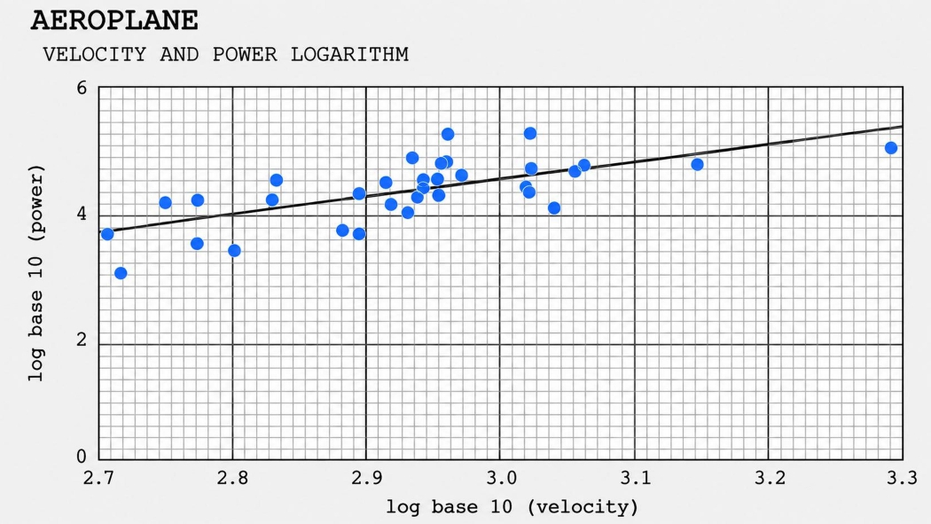
y = 2.8315x − 3.9878
UAV
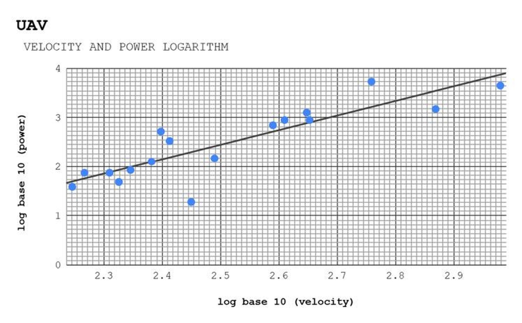
y = 2.9625x − 4.9595
Battery drones
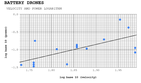
y = 2.7068x − 5.9992
Interpretation
The following tables gives all the data regarding the regression lines (equation 9,10, and 11) and hence the following data is used for further discussion:
| Subject | Regression equation |
| Aeroplanes | y = 2.8315x − 3.9878 |
| UAVs | y = 2.9625x − 4.9595 |
| Battery drones | y = 2.7068x − 5.9992 |
| r | r² | b (Slope) | ε + C (Constant) |
| 0.6817 | 0.4647 | 2.8315 | −3.9878 |
| 0.8671 | 0.7518 | 2.9625 | −4.9595 |
| 0.6920 | 0.4789 | 2.7068 | −5.9992 |
The equation of the trendline is given in the y-intercept form, i.e. where  and
 are the slope and the y-intercept. The graphs of the aerial vehicles’ data show the relationship between power and velocity in mechanics through logarithms. It could be observed in all three graphs that the points are close enough to apparently show the that the points are showing an upward trajectory, hence we use a trendline which makes the graph linear, bringing wide ranges of data to a smaller comparable scale using logarithms and bring wide ranges to a smaller comparable scale. The whole dataset on the graph is interpreted using the leastsquares regression line, as it is obtained by minimizing the sum of squared deviations of data points from the line, which represents the whole dataset, thus giving the trajectory of the data points, which is calculated using the least squares linear regression formula.
Correlation coefficient (r): 0.0, No correlation; Correlation coefficient (r): 0.3, Weak positive correlation; Correlation coefficient (r): 0.5, Moderate positive correlation; Correlation coefficient (r): 0.7, Strong positive correlation; Correlation coefficient (r): 1.0, Perfect positive correlation. Using the mentioned scale to examine the corelation of the aircrafts’ dataset.37
Aeroplanes have a correlation coefficient (r) of 0.6817, indicating a moderate positive correlation that is close to strong. UAVs have a correlation coefficient (r) of 0.8671, indicating a strong positive correlation. Battery drones have a correlation coefficient (r) of 0.6920, indicating a moderate positive correlation that is close to strong.
The strength of the relationship between two variables can be assessed by evaluating the numerical value of the correlation coefficient. Correlation values can range from -1 to +1. In the following case the two variables are the data point and regression line.
‘r2’is the derived value of the corelation coefficient which is positive without any manipulation. ‘b’ is the slope of the least square regression line of the scattered data points of the aircrafts’ logarithmic values of power and velocity. It is derived by comparing the general y intercept to the equation made for further examination.
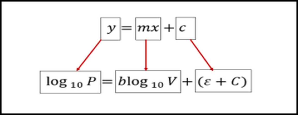
It is the major quantity which helps us to examine the cubic law as it compares the exponents of the two quantities. Hence,
should be equal to three.
The regression slopes approach the theoretical cubic scaling exponent, although systematic deviations are evident. As fore mentioned in the table: 2.8315, 2.9625, 2.7068
Why is the regression slope not exactly equal to 3?
For steady flight,  and
 .
 represents propulsive efficiency38:
It is the propeller efficiency as the ratio of useful thrust power to engine brake power.
Since  , the ideal relation becomes
therefore, 
An exact slope of 3 requires , ,  , and propulsion efficiency to remain constant. In real aerial vehicles, these parameters vary with altitude, configuration, payload, propulsion type, and flight condition. Hence, the observed slopes 2.8315, 2.9625, and 2.7068 approach, but do not exactly equal to 3 as per the theoretical cubic exponent.
Constant interpretation
The term + C represents the y-intercept and determines the vertical or multiplicative scale of the power–velocity relationship. as defined earlier in equation7 and equation8. as defined earlier under equation 5. Since  from equation 6 taking the inverse logarithm gives
Therefore, + C determines the multiplicative scale of power, while b determines how rapidly power changes with velocity. A larger intercept produces a higher predicted power at the same velocity, whereas a smaller intercept shifts the regression line downward.
Discussion
The following work is both interesting and important, as it investigates a scaling law, derived from the mechanics branch of physics, that expresses a cubic relationship between power and velocity using data from real aircraft, neither estimated nor idealized.
The relation broadly explains the fundamental reasons behind the design and modelling of aircraft propulsion systems and how different factors affect the aerodynamics of vehicles, especially aerial vehicles. The work leads us to study its application across many branches of engineering. It explains how power consumption by the propulsion systems varies with velocity. The log-log plot shows a linear trend to make the study comparable and scalable, making it easier to analyse the exponential relationship with a trendline. This also reveals different intercepts representing different ‘aerodynamic/propulsive fingerprints’ across vehicle classes. It proves the relationship between power and velocity using logarithms and a graphical approach and provides a detailed theoretical proof of the relationship and the line’s equation, along with interpretations of other factors. Surprisingly, the aircraft used in World Wars I and II show the same relationship as modern aircraft. Even after such technological advancement, the same relationship is observed between batteries and aeroplanes, despite the aeroplanes being more than 70 times larger, thus proving that physics neither fails nor compromises. The lower slope indicates advanced aerodynamics, as seen in the UAV graph, whereas the aeroplanes have the highest slope, indicating slightly less efficient aerodynamics than battery drones and UAVs. The same concept is used in Formula One racing, the slipstreaming effect, in which F1 car behind another car performs better due to less aerodynamic drag force.Hence, the thing that makes this paper important is its countless applications in several branches of engineering, especially aerospace, mechanical, and automobile engineering, which is also proved by this paper by plotting a log-log graph of power and velocity of an aerial vehicle, which ultimately proves the cubic relationship.39
Future Work
This work has strong potential for real-world application across multiple branches of engineering. By leveraging the cubic relationship between power and velocity, it enables estimation of energy or fuel requirements for aerial vehicles operating at specific speeds, helping identify optimal and energy-efficient flight regimes. The results can inform the design of more aerodynamically efficient and cost-effective aircraft, particularly for long-duration missions involving UAVs, battery-powered drones, and high-endurance platforms. Beyond design and performance prediction, this study provides a practical framework for teaching fundamental concepts in aerodynamics and mechanics through real-world data. The established relationship can also be used to predict unknown performance parameters of existing or future vehicles with minimal experimental effort. Furthermore, incorporating altitude-dependent air density effects offers a natural extension of this work, enabling improved analysis of flight performance across operational altitudes. Finally, since the same cubic scaling governs wind energy extraction, the methodology is directly applicable to evaluating wind turbine efficiency, extending the relevance of this study beyond aviation into renewable energy systems.
Conclusions
This study empirically investigates the power-velocity relationship across aeroplane, engine driven UAV and battery drones using logarithmic relationship between publicly available specification of the involved quantities i.e. power and velocity. The subsequent datapoints were plotted scattered on graph to obtain a trendline. On comparison with the y-intercept form of line, the fitted slopes were 2.8315, 2.9625, and 2.7068 for aeroplanes, UAVs, and battery drones, respectively, with corresponding correlation coefficients of 0.6817, 0.8671, and 0.6920 and coefficients of determination of 0.4647, 0.7518, and 0.4789. The results indicate that the cubic power-velocity relationship provides a suitable first-order description of power scaling across aerial vehicles spanning extensively over different sizes, propulsion systems, and operating speeds. The regression slopes approach the theoretical cubic scaling exponent, granting systematic deviations are apparent. The near-cubic slopes encourage the theoretical expectation that parasite-drag power becomes progressively significant as velocity increases. The study exhibits that logarithmic regression can be used to compare power-law behaviour across diverse aerial-vehicle categories using real specification data. The findings may support preliminary performance comparison, propulsion analysis, engineering education, and the identification of vehicle categories requiring more detailed aerodynamic modelling. The primary objective of evaluating whether empirical aerial-vehicle data follow an approximately cubic power-velocity trend was substantially achieved. The results support approximate cubic scaling rather than exact equivalence to the theoretical exponent thus supporting the apparent uncertainties in the test of power and velocity. The findings do not constitute controlled experimental verification because the collected values were obtained from non-uniform sources and operating conditions. Published maximum power and velocity values were often stated under different operating states and were not necessarily measured simultaneously. In addition, the datasets combined non-equivalent power definitions, including thrust-derived power, shaft power, rated motor power, and avg. battery power, which limits direct cross-category comparison and introduces uncertainty into the fitted relationship. Overall, the study identifies a measurable near-cubic power-velocity trend across real aerial-vehicle categories despite substantial differences in design, and operating conditions. The findings provide exploratory empirical support for the theoretical cubic scaling law, while emphasizing that standardized, simultaneous, and controlled measurements are necessary for rigorous experimental validation.
Appendix
References
- W. M. Saslow. A history of thermodynamics: the missing manual. Entropy. Vol. 22, pg. 77, 2020 https://doi.org/10.3390/e22010077 [↩] [↩]
- A. Gilam. The technology of air power during the great war. Computers & Mathematics with Applications. Vol. 26, pg. 149–152, 1993 https://doi.org/10.1016/0898-1221(93)90124-E [↩]
- Janusz Nowotny, T. Nejat Veziroglu. International journal of hydrogen energy. Vol. 36, pg. 13218–13224, 2011 https://doi.org/10.1016/j.ijhydene.2011.07.071 [↩]
- J. Peksa. A review on the state of the art in copter drones and flight control systems. Sensors. Vol. 24, pg. 3349, 2024 https://doi.org/10.3390/s24113349 [↩] [↩]
- El-Sayed, Ahmed F. Fundamentals of Aircraft and Rocket Propulsion. London, 2016 [↩] [↩]
- Y. Zeng, R. Zhang. Energy-efficient uav communication with trajectory optimization. IEEE Transactions on Wireless Communications. Vol. 16, pg. 3747–3760, 2017 https://doi.org/10.1109/twc.2017.2688328 [↩]
- Y. Zeng, J. Xu, R. Zhang. Energy minimization for wireless communication with rotary-wing uav. IEEE Transactions on Wireless Communications. Vol. 18, pg. 2329–2345, 2019 https://doi.org/10.1109/twc.2019.2902559 [↩] [↩]
- J. K. Stolaroff, C. Samaras, E. R. O’Neill, A. Lubers, A. S. Mitchell, D. Ceperley. Energy use and life cycle greenhouse gas emissions of drones for commercial package delivery. Nature Communications. Vol. 9, pg. 409, 2018 https://doi.org/10.1038/s41467-017-02411-5 [↩]
- A. Zhao, J. Zhang, K. Li, D. Wen. Design and implementation of an innovative airborne electric propulsion measure system of fixed-wing uav. Aerospace Science and Technology. Vol. 109, pg. 106357, 2021 https://doi.org/10.1016/j.ast.2020.106357 [↩]
- T. A. Rodrigues, J. Patrikar, A. Choudhry, J. Feldgoise, V. Arcot, A. Gahlaut, S. Lau, B. Moon, B. Wagner, H. S. Matthews, S. Scherer, C. Samaras. In-flight positional and energy use data set of a dji matrice 100 quadcopter for small package delivery. Scientific Data. Vol. 8, pg. 155, 2021 https://doi.org/10.1038/s41597-021-00930-x [↩] [↩]
- C. Zhang, C. Zhang, L. Li, Q. Guo. Parameter analysis of power system for solar-powered unmanned aerial vehicle. Applied Energy. Vol. 295, pg. 117031, 2021 https://doi.org/10.1016/j.apenergy.2021.117031 [↩]
- G. Aiello, K. P. Valavanis, A. Rizzo. Fixed-wing uav energy efficient 3d path planning in cluttered environments. Journal of Intelligent & Robotic Systems. Vol. 105, pg. 60, 2022 https://doi.org/10.1007/s10846-022-01608-1 [↩]
- L. Bauersfeld, D. Scaramuzza. Range, endurance, and optimal speed estimates for multicopters. IEEE Robotics and Automation Letters. Vol. 7, pg. 2953–2960, 2022 https://doi.org/10.1109/lra.2022.3145063 [↩]
- T. A. Rodrigues, J. Patrikar, N. L. Oliveira, H. S. Matthews, S. Scherer, C. Samaras. Drone flight data reveal energy and greenhouse gas emissions savings for very small package delivery. Patterns. Vol. 3, pg. 100569, 2022 https://doi.org/10.1016/j.patter.2022.100569 [↩]
- H. Zhang, S. Tan, Z. Song, Q. Quan. Performance evaluation and design method of lifting-wing multicopters. IEEE/ASME Transactions on Mechatronics. Vol. 27, pg. 1606–1616, 2022 https://doi.org/10.1109/tmech.2021.3090667 [↩]
- M. Carreño Ruiz, M. Scanavino, D. D’Ambrosio, G. Guglieri, A. Vilardi. Experimental and numerical analysis of hovering multicopter performance in low-reynolds number conditions. Aerospace Science and Technology. Vol. 128, pg. 107777, 2022 https://doi.org/10.1016/j.ast.2022.107777 [↩]
- K. Góra, P. Smyczyński, M. Kujawiński, G. Granosik. Machine learning in creating energy consumption model for uav. Energies. Vol. 15, pg. 6810, 2022 https://doi.org/10.3390/en15186810 [↩]
- L. Zhu, Z. Xu, Y. Wang, C. Cheng. Correlation analysis of energy consumption of agricultural rotorcraft. Computers, Materials & Continua. Vol. 71, pg. 3179–3192, 2022 https://doi.org/10.32604/cmc.2022.023293 [↩]
- X. Dai, B. Duo, X. Yuan, W. Tang. Energy-efficient uav communications: a generalized propulsion energy consumption model. IEEE Wireless Communications Letters. Vol. 11, pg. 2150–2154, 2022 https://doi.org/10.1109/lwc.2022.3195787 [↩]
- H. Gong, B. Huang, B. Jia, H. Dai. Modeling power consumptions for multirotor uavs. IEEE Transactions on Aerospace and Electronic Systems. Vol. 59, pg. 7409–7422, 2023 https://doi.org/10.1109/taes.2023.3288846 [↩]
- M. Żugaj, M. Edawdi, G. Iwański, S. Topczewski, P. Bibik, P. Fabiański. An unmanned helicopter energy consumption analysis. Energies. Vol. 16, pg. 2067, 2023 https://doi.org/10.3390/en16042067 [↩]
- R. Głębocki, M. Żugaj, M. Jacewicz. Validation of the energy consumption model for a quadrotor using monte-carlo simulation. Archive of Mechanical Engineering. Vol. 70, pg. 151–178, 2023 https://doi.org/10.24425/ame.2022.144075 [↩]
- N. Han, M. A. Siddique, Z. Zhang, L. Tian, H. Hu, H. Hu. A flight-testing campaign to examine inflight icing characteristics and its effects on the flight performance of an unmanned-aerial-vehicle. Cold Regions Science and Technology. Vol. 207, pg. 103775, 2023 https://doi.org/10.1016/j.coldregions.2023.103775 [↩]
- J. Van Mulders, J. Cappelle, S. Goossens, L. De Strycker, L. Van der Perre. UAV-based servicing of iot nodes: assessment of ecological impact. Sensors. Vol. 23, pg. 2291, 2023 https://doi.org/10.3390/s23042291 [↩]
- A. Mohiuddin, T. Taha, Y. Zweiri, D. Gan. Dual-uav payload transportation using optimized velocity profiles via real-time dynamic programming. Drones. Vol. 7, pg. 171, 2023 https://doi.org/10.3390/drones7030171 [↩]
- W. Dai, M. Zhang, K. H. Low. Data-efficient modeling for power consumption estimation of quadrotor operations using ensemble learning. Aerospace Science and Technology. Vol. 144, pg. 108791, 2024 https://doi.org/10.1016/j.ast.2023.108791 [↩]
- U. C. Çabuk, M. Tosun, O. Dağdeviren, Y. Ozturk. Modeling energy consumption of small drones for swarm missions. IEEE Transactions on Intelligent Transportation Systems. Vol. 25, pg. 10176–10189, 2024 https://doi.org/10.1109/tits.2024.3350042 [↩]
- A. Ait Saadi, B. P. Bhuyan, A. Ramdane-Cherif. Power consumption model for unmanned aerial vehicles using recurrent neural network techniques. Aerospace Science and Technology. Vol. 157, pg. 109819, 2025 https://doi.org/10.1016/j.ast.2024.109819 [↩]
- E. I. Abd El-Latif, M. El-dosuky. Predicting power consumption of drones using explainable optimized mathematical and machine learning models. The Journal of Supercomputing. Vol. 81, pg. 646, 2025 https://doi.org/10.1007/s11227-025-07105-0 [↩]
- M. Kim, M. Kim, Y. Chen, J. Kim, D. Baek. Hybrid dnn-based flight power estimation framework for unmanned aerial vehicles. Drones. Vol. 9, pg. 104, 2025 https://doi.org/10.3390/drones9020104 [↩]
- W. Li, R. Cheng, H. Huang, A. Garg, L. Gao. Energy consumption modeling and optimization of an evtol aircraft: integrating weight, motor, and battery dynamics. Energy. Vol. 325, pg. 136229, 2025 https://doi.org/10.1016/j.energy.2025.136229 [↩]
- E. Ntouros, P. Kelley, E. J. J. Smeur. Airspeed estimation for uavs using only propeller feedback. Aerospace Science and Technology. Vol. 168, pg. 110999, 2026 https://doi.org/10.1016/j.ast.2025.110999 [↩]
- P. Bauer. A modified total energy control scheme for unmanned aircraft. Journal of Intelligent & Robotic Systems. Vol. 109, pg. 66, 2023 https://doi.org/10.1007/s10846-023-01998-w [↩]
- S. Maxemow. That’s a drag: the effects of drag forces. Undergraduate Journal of Mathematical Modeling: One + Two. Vol. 2, pg. 1–16, 2009 https://doi.org/10.5038/2326-3652.2.1.4 [↩]
- National Aeronautics and Space Administration. Size effects on drag. 2024 [↩] [↩]
- Gurrola Arrieta, M. de J., Botez, R. M. A methodology to determine the precision uncertainty in gas turbine engine cycle models. The Aeronautical Journal. Vol. 128, pg. 92–110, 2024 https://doi.org/10.1017/aer.2023.64 [↩] [↩]
- National University. Correlation. [↩]
- Federal Aviation Administration. Chapter 7. in Federal Aviation Administration, Washington, DC [↩]
- X. Liu, A. Fotouhi, M. Cecotti, D. Auger. Optimal control of race car with aerodynamic slipstreaming effect. IEEE Transactions on Control Systems Technology. Vol. 32, pg. 2136–2148, 2024 https://doi.org/10.1109/TCST.2024.3395722 [↩]