Monitoring Sand Boils to Prevent Levee Failures Using Machine Learning

Abstract

Most levees in California are old structures, many of which were originally built in the 1800s and are now vulnerable to collapse. In response to growing concerns about their integrity, the state has issued a mandate requiring that levees in high-risk areas be upgraded by 2030. One of the primary threats to levee stability is the occurrence of sand boils, which emerge when pressurized water forces its way to the surface, and can lead to sudden and catastrophic collapses. To investigate the feasibility of automating the visual detection of sand boils in images, we evaluated deep learning image segmentation models trained on a limited AI generated dataset. Specifically, we trained and evaluated U-Net models including a baseline Convolutional Neural Network U-Net, a Swin Transformer U-Net, and an EfficientNet-B4 U-Net. The models demonstrated strong performance, showing promise as an initial algorithmic approach for automated levee monitoring systems. After evaluating multiple state-of-the-art U-Net segmentation models, a U-Net with an EfficientNet B4 backbone achieved a dice score of 65.08% and an Intersection over Union (IoU) of 53.36% on the held-out test set. The model’s predictions were able to capture the exact, complex contours of the sand boils. While restricted to controlled experimental conditions,this project also shows that machine learning models can learn effective sand boil segmentation capabilities from only 51 real examples, even when limited to 2D photos and U-Net architectures. Early detection of sand boils can significantly reduce the risk of levee breaches and enhance the resilience of flood protection infrastructure.

Keywords: Sand Boils, Levee Monitoring, Deep Learning, Image Segmentation, U-Net Architecture, EfficientNet, Synthetic Data, Data Scarcity

Introduction

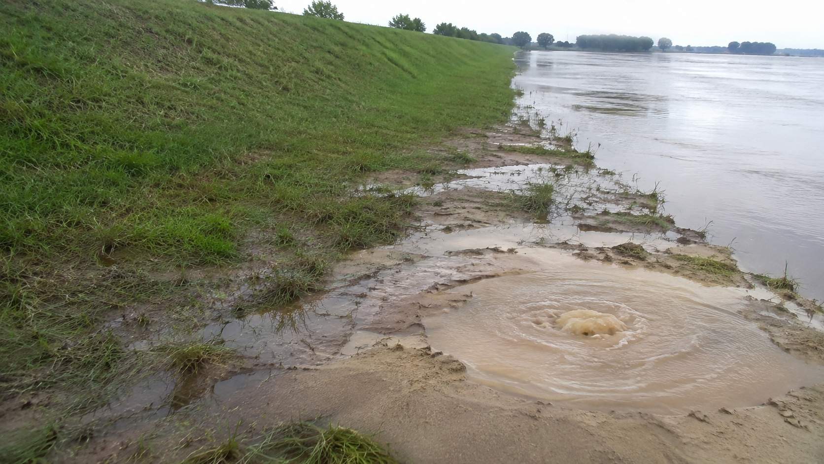
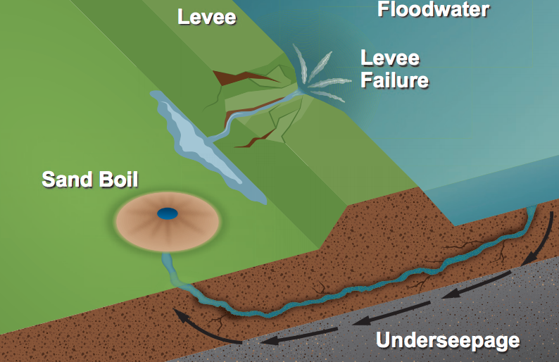
A levee is a large structure typically built around cities near a water source to prevent flooding. Levees are designed to provide a certain level of protection against flooding events; however, they require constant maintenance and monitoring, as severe weather conditions and earthquakes can damage them¹. Sand boils are one of the biggest threats to these levees². A sand boil is a geological phenomenon that occurs when water under pressure forces its way to the surface, carrying sand and silt with it, creating a small cone or “boil” of sediment, as demonstrated in Fig. 1³.

Sand boils typically happen during flooding or in areas with high groundwater pressure, especially when water seeps through levees, embankments, or other earth structures. The upward flow of water weakens the soil’s strength, and if unchecked, sand boils can lead to serious erosion or even structural failure of levees and dams⁴. Sand boils are a warning sign of potential soil instability and are closely monitored in flood-prone regions to prevent breaches or collapses. Detecting sand boils manually for levee protection has been labor-intensive and challenging⁵.

The Central Valley Flood Protection Act requires high-risk areas in California to achieve a 200-year flood protection standard⁶. This is becoming increasingly important due to climate change. There have been stronger atmospheric rivers in California, which can create massive floods, causing even more levee instability⁷. To overcome this issue, we hypothesized that a U-Net segmentation model trained on synthetic data can automate sand boil detection with a dice score of greater than 60 percent, significantly reducing the manual inspection time while maintaining high spatial accuracy. This research aims to help with levee and sand boil monitoring and improve the safety of the cities near bodies of water in high-risk zones. To test our hypothesis, we developed several U-Net models to segment images of sand boils from an AI-generated dataset, enabling early detection and intervention.

In recent years, advances in Artificial Intelligence (AI) have enabled researchers to tackle similarly exigent environmental problems. An example is how deep learning was used to predict impending forest fires⁸ and identify their locations. Segmentation models can be utilized to identify areas that are more prone to fire and where conditions are favorable for wildfires. AI is also being applied to hurricane forecasting, checking maps of wind conditions, analyzing wind patterns, and humidity levels⁹. These studies demonstrate how AI can accelerate the solution to many persistent environmental problems when sufficient data is available for analysis and training.

Prior work on levee monitoring has demonstrated the viability of AI in this domain. For instance, Kuchi et al. (2019) explored machine learning applications for detecting sand boils from images, treating it as a central detection task¹⁰. However, little research exists on levee monitoring, particularly sand boil detection. This is, in part, due to the lack of public, robust sand boil data. With only 51 real-world images available in our dataset, data scarcity has become a significant roadblock in the implementation of machine learning (ML) models. To address the data scarcity gap, the model was trained on synthetically generated images created with DreamBooth’s open-source diffusion model¹¹. Although this introduces some data leakage in the dataset, all new images of sand boils were carefully reviewed to ensure they are realistic and that no generated images are similar to the original ones.

Building upon these foundations, this research specifically investigates whether deep learning segmentation models can successfully identify sand boils when trained on a limited dataset augmented by DreamBooth synthetic imagery. In this project, we programmed an automated system to train, test, and compare three different U-Net deep learning models to select the best performer to identify and precisely locate sand boils in 2D images. This study acts as a preliminary comparison of U-Net architectures under data-scarce conditions. The scope of this study is strictly limited to 2D image segmentation on static photographs and does not currently encompass real-time video processing, drone deployment, or physical size estimation.

Methods

The dataset used for this project is from IEEE Dataport, “Synthetic Sand Boil Dataset for Levee Monitoring”¹². The dataset includes 930 training images (approximately 94.8% of the total images) with corresponding masks for sand boils, synthetically generated using DreamBooth’s open-source diffusion model. The dataset also provides 51 real images of sand boils along with their human-annotated masks. These images are labeled for a validation set, not for testing. Out of the 51 real images, 10 images (approximately 1.0%) were set aside to tune the hyperparameters, and the remaining 41 (approximately 4.2%) were used for testing. Each image is approximately 400 KB, resulting in a total dataset size of 381 MB.

To ensure no data leakage occurred from the DreamBooth generation, a quantitative nearest-neighbor analysis was performed comparing the 41 real test images against the synthetic training set using both raw pixel similarity and internal feature representations. No synthetic training images closely matched the real test images (the highest recorded cosine similarity score between any synthetic training image and a real test image was 0.9281, with a mean maximum similarity of 0.8287, quantitatively confirming the absence of exact duplicates). Additionally, we used a negative cohort of 23 images containing intact levees, clear-water seepage, puddles, and bare soil to test the model’s false-positive rate and specificity in cluttered environments.

During training, images were augmented with random reflections (50% of the time) and brightness adjustments (20% of the time). These specific techniques were chosen to counteract the static nature of the synthetic dataset; brightness adjustments simulate diverse levee lighting conditions (e.g., overcast versus bright sunlight), while random reflections ensure the model remains invariant to camera orientation, ultimately reducing false positives.

Baseline U-Net

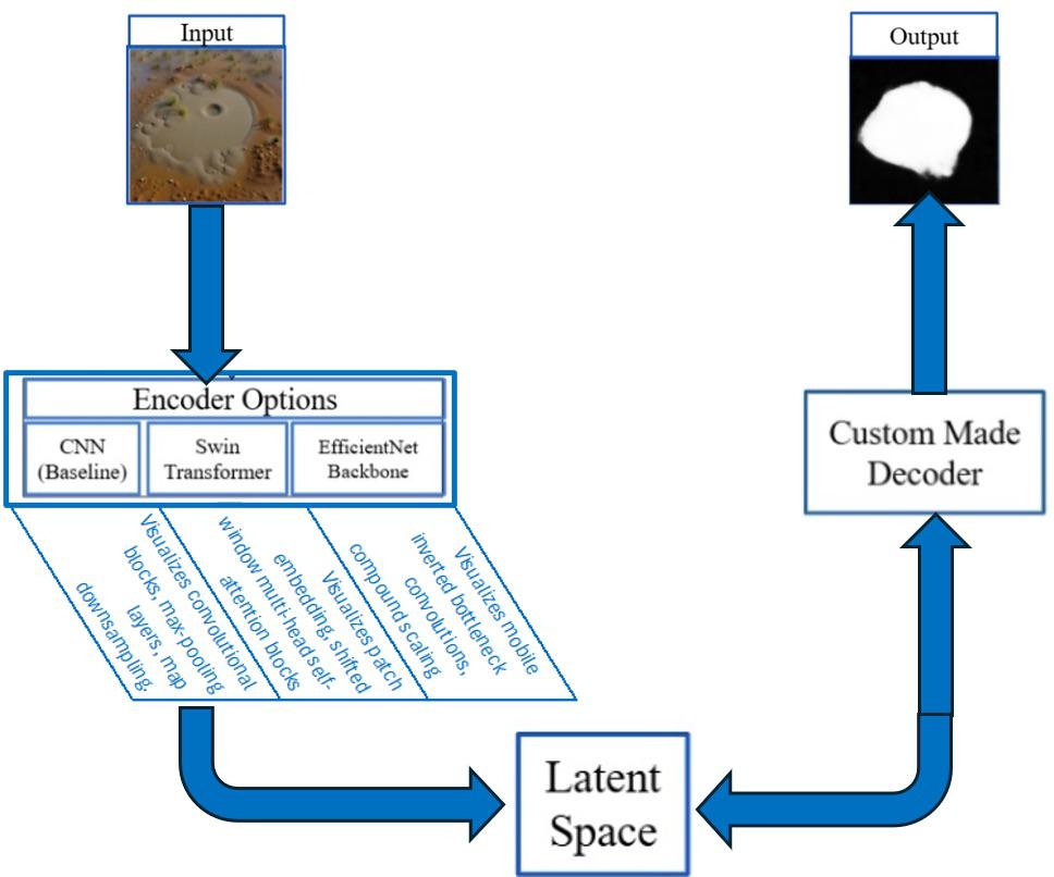
We chose the U-Net architecture from Fig. 2 for the initial Sand Boil dataset segmentation due to its demonstrated efficacy in extracting edge details from limited, high-contrast imagery in medical and geological domains for segmentation tasks. Our study focuses on optimizing encoder backbones within the U-Net architecture to determine the most parameter-efficient feature extractor for sand boil segmentation.

U-Nets work through layers of encoders and decoders that detect pixels in the image and determine if they are part of what the model is looking for¹³. The encoders transform the image signal into a lower-dimensional representation called the latent space, as referenced in Fig. 2. The decoders then decode the lower-dimensional signal back to the dimensions of the original image to generate a mask for the desired object. The baseline U-Net in this project employs a convolutional neural network backbone (CNN)¹⁴.

U-Net with Swin Transformer Backbone

To improve the segmentation performance of the baseline U-Net model, newer state-of-the-art backbones like the Swin U-Net were also explored.

A Swin U-Net is a type of deep learning model that combines the extraction of the Swin transformer with the encoder-decoder architecture of the U-Net, which is widely used for image segmentation. In this hybrid model, the Swin transformer replaces the standard convolutional blocks in both the encoder and decoder paths, enabling the network to capture both local and global context through self-attention mechanisms with shifted windows. This design allows the Swin U-Net to process images at multiple scales while maintaining computational efficiency effectively¹⁵. The architecture is particularly well-suited for tasks like medical image segmentation, where detailed spatial understanding and context awareness are crucial. Applying this approach to sand boil images helps to address the complexity of the levee context in actual delta field conditions. Sand boils may appear very small within wide, cluttered, and messy images or be partially obscured by vegetation, shadows, or surface debris.

U-Net with EfficientNet Backbone

Another useful model backbone for this task is EfficientNet. EfficientNet is a family of convolutional neural network models developed by Google that aim to achieve high accuracy while being computationally efficient. Introduced in 2019, it uses a new compound scaling method to systematically scale the model’s depth, width, and resolution in a balanced way, rather than arbitrarily increasing just one of them. At its core, EfficientNet is built upon a baseline model called EfficientNet-B0, which was optimized using neural architecture search. Larger versions, B1 to B7, were created by uniformly scaling the network. Compared to traditional models like ResNet¹⁶ or VGG¹⁷, EfficientNet achieves better accuracy with significantly fewer parameters and lower computational cost¹⁸. Among all these models used in this research, the EfficientNet-B4 model outperforms other U-Net models in sand boil segmentation.

The U-Net models were trained in a Google Colab Notebook environment using an Nvidia Tesla T4 GPU with 15 GiB of memory. In terms of computational complexity, the EfficientNet-B4 U-Net utilizes approximately 19 million parameters and requires ~15 GFLOPs per image. This optimized architecture allows it to fit comfortably within the 15 GiB memory limit of the Tesla T4 GPU, requiring only 45 minutes for the 25-epoch training cycle. This efficiency demonstrates its viability for eventual real-time inference on edge devices, achieving an inference time of less than 0.4 seconds per image and fitting the space requirements to run even on a small device.

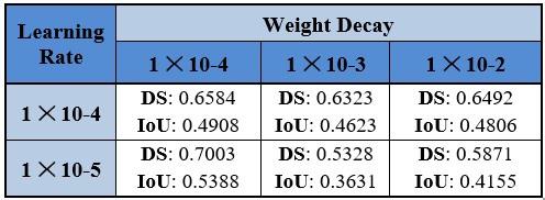
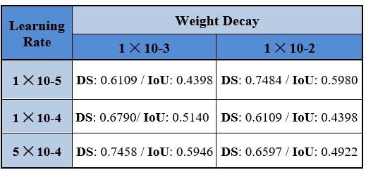
The learning rates and weight decay for each model have been tuned on the validation set. 15 targeted ablation experiments were conducted to establish this final hyperparameter configuration. Furthermore, a patience value of 3 epochs was utilized for the learning rate scheduler and early stopping criterion to improve training stability and reproducibility.The batch size for training is 8 to accommodate GPU memory limits while providing reliable gradient estimates. The model uses the AdamW optimizer¹⁹ from the PyTorch library. Unlike standard L2 regularization, AdamW decouples weight decay from the gradient updates, shrinking the model’s parameters directly at each step to effectively prevent overfitting and improve generalization on our small dataset.

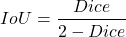
A dice score was used to evaluate model performance on this task. Dice score is an indicator of the pixel-wise overlap between the predicted object  and the actual object y, in this case, the sand boil²⁰. The dice score is calculated as in formula (1):

(1)  

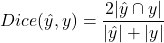
Note that  is the number of pixels in the object , |y| is the number of pixels in the object y, and |∩y| is the number of pixels in common between the two objects. A combined loss was also used in this model, combining binary cross-entropy loss and dice loss together. This specific combination was selected because BCE provides stable, smooth gradients for pixel-wise classification, while the Dice loss directly optimizes our primary evaluation metric and effectively mitigates the severe class imbalance (small sand boils versus large levee backgrounds) without requiring the additional complex hyperparameter tuning associated with Focal²¹ or Tversky²² loss.

(2)  

As shown in formula (2), dice loss is simply 1 minus the dice score. The binary cross-entropy formula is demonstrated below, as in formula (3) for one sample and as in formula (4) for N samples:

One Sample:

(3)  

N Samples

(4)  

Note that y is the true label, which is either 0 or 1, and p is the predicted probability that y is 1 from a sigmoid function. The combined loss now takes both of these two loss functions and adds them together based on a new coefficient α.

(5)  

As demonstrated in formula (5), α is usually chosen to be  to combine both losses equally, and  is derived from p, whereas if p>0.5, then =1, and if p<0.5, then.

Results

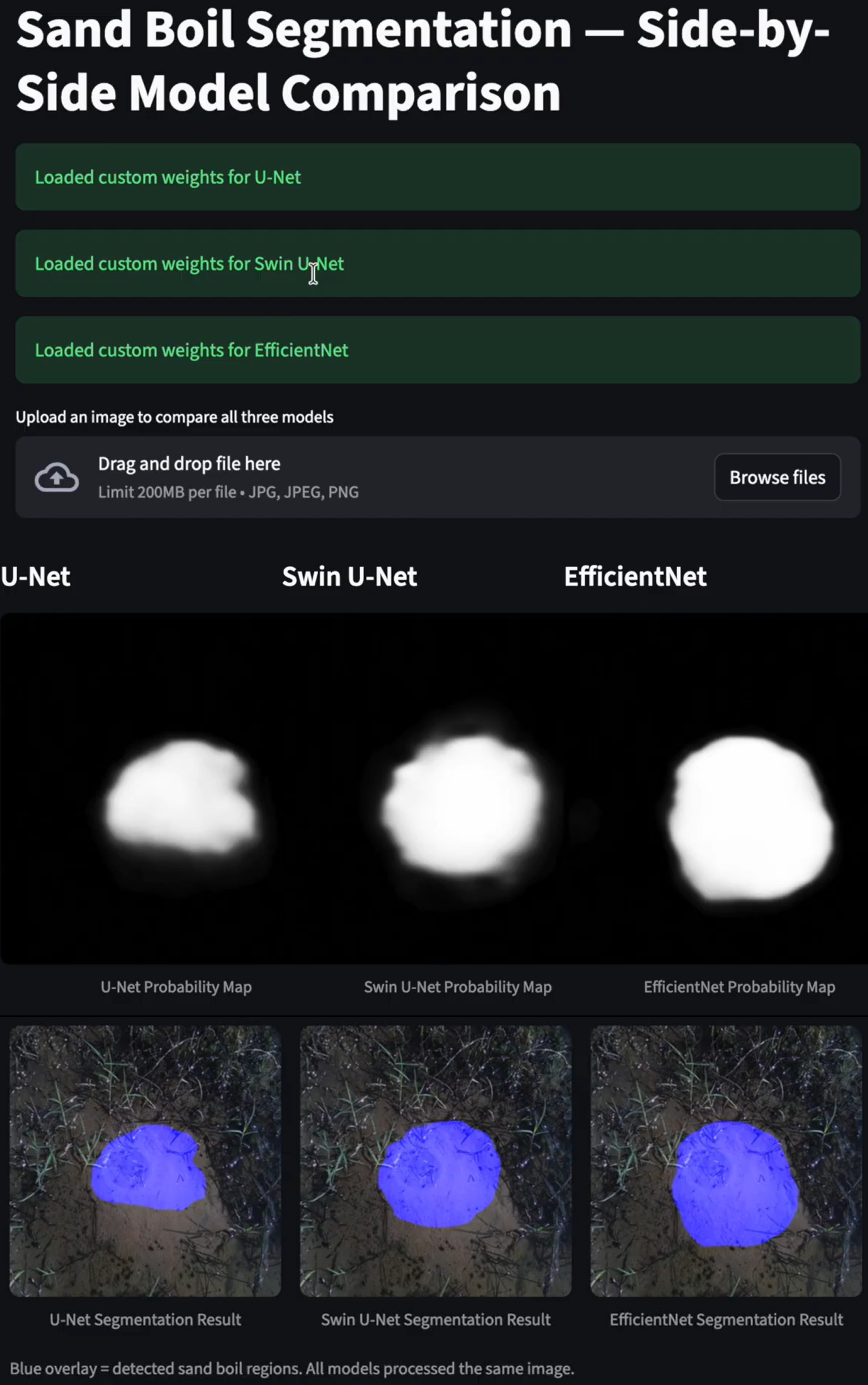
During the testing of the models, 25 epochs were used to train the model, and using the dice score as a training metric gave a better dice score result. The model was saved at the epoch with the best validation metric, which was subsequently used for testing. Experiments were done using the best loss or the best dice to select which epoch to save the model, as demonstrated in Table 3. The baseline U-Net model had a 58.35% dice score on the test set when the best loss was used, and a 55.76% dice score on the test set when the best dice score was used. Additionally, this baseline model yielded a Mean Intersection over Union (IoU) of 48.71%, a Mean Precision of 65.06%, and a Mean Recall of 62.12%. The Swin U-Net model, however, had a 56.73% dice score on the testing set when the best loss was used, and a 59.33% dice score on the testing set when the best dice score was used. Additionally, the Swin U-Net model yielded a Mean Intersection over Union (IoU) of 52.95%, a Mean Precision of 64.13%, and a Mean Recall of 74.45%. The EfficientNet B4 model, surpassing all the others, had a 64.85% dice score on the testing set when the best loss was used, and a 65.08% dice score on the testing set when the best dice score was used. Furthermore, the EfficientNet B4 model achieved a Precision of 63.75%, a Mean Recall of 73.41%, and an Intersection over Union (IoU) of 53.36%, with a standard deviation of 0.0039 confirming performance stability. Testing on the negative cohort (images without sand boils) produced a true-negative of 69.23% and a false-positive rate of 30.77%, demonstrating the model’s baseline ability to distinguish sand boils from similar soil features.

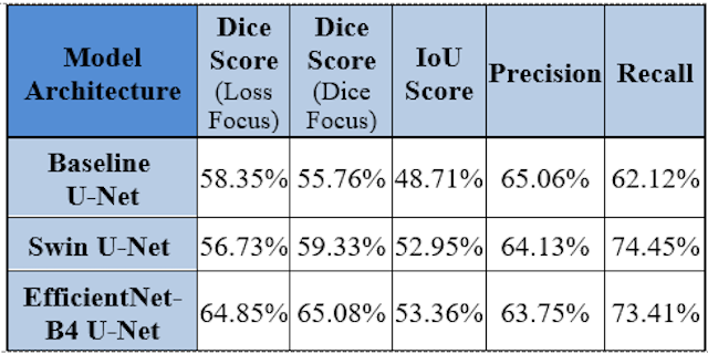
EfficientNet-B4 architecture performed better than the baseline U-Net and Swin U-Net because its compound scaling method captures both fine-grained sand boil details and broader levee context simultaneously. While the baseline U-Net cannot handle such complex extraction and the Swin Transformer requires more data than we have available, EfficientNet scales width, depth, and resolution effectively for this data-scarce environment.

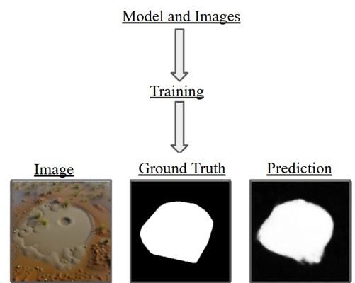
One interesting qualitative observation of this model is its ability to create segmentations with smooth boundaries, which differ from the simplified geometric annotations of the manual ground truth masks. The ground truth masks weren’t very accurate to its true shape. As illustrated in Fig. 3, the prediction mask is a lot more reflective of the original image than the simplified geometric annotations of the manual ground truth masks provided by the dataset. Having a more detailed segmentation shape would be even more helpful for the model, as it would allow it to make a more accurate size calculation. Since the ground-truth annotations serve as our reference standard, the 65.08% dice score specifically reflects the overlap with our current ground-truth annotations.

Discussion

This model achieved a high dice score of 65.08% on the testing set, which demonstrates this approach as a promising initial algorithmic approach in monitoring levee safety. It is important to note that the dice score is not equivalent to accuracy. Given the imperfect ground-truth labels, a 65.08% dice score enabled capturing the overall shape of the sand boils; therefore, the score is considered good for this type of model. This seemingly modest 65.08% ceiling is primarily driven by two factors: the severe domain gap between the synthetic training data and the real-world test data, and the heavily simplified geometric nature of the manual annotations, which artificially penalize the model’s score when it predicts a genuinely correct but highly complex, diffuse boundary.

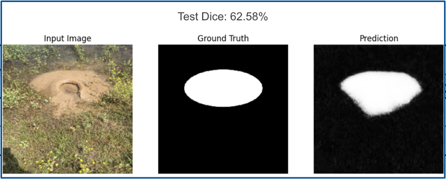
As shown in Fig. 4, even at a dice score of 62.58%, which is less than our best performance, the model can output detailed masks better than the ground truth and capture the exact contours of the sand boils.

A systematic error analysis was conducted to identify the framework’s limitations and provide a more objective evaluation. While the model accurately identifies distinct, high-contrast sand boils, it struggles with low-quality images, complex backgrounds, such as over-segmenting mud puddles that mimic boil textures or under-segmenting boils obscured by dense vegetation.

While EfficientNet has proven a great ability for sand boil segmentation, the training pipeline has faced several limitations. The main limitation of this study is the small evaluation set. The dataset provided was small, with fewer than 1000 images in total for training and validation combined. Testing images were not included. The validation set was also limited, as the original dataset only included 51 images for validation. These images were then split to form 10 for the new validation set and 41 for the test set, which made them even smaller than before. Consequently, the results should be interpreted as an initial feasibility assessment of sand boil segmentation under severe data constraints. As illustrated in Fig. 3 and Fig. 4, the ground truth masks for the provided images also lacked detail and proper shape, most of them being basic ellipses. Despite the low quality of the ground truth masks, the reported Dice score (65.08%) and IoU score (53.36%) demonstrate that the EfficientNet-B4 U-Net consistently identifies the boundaries of sand boil features, even with significant differences between synthetic training data and real-world conditions, such as weather fluctuations, illumination, vegetation obstructions, different camera angles, or motion blur.

Another limitation was that the majority of the dataset was synthetic, and the creators did not disclose their methods for generating these images, meaning data leakage could be possible.

To address current data constraints, improve model independence, and enhance practical relevance, our future work will expand the dataset by simulating diverse real-world environmental factors, implementing active learning annotation pipelines, and evaluating alternative non-U-Net architectures, such as combining an EfficientNet model with a Mask R-CNN (Region-based Convolutional Neural Networks)²³. In this integrated system, Mask R-CNN would perform the initial broad-area detection to efficiently scan large levee sectors and generate bounding boxes around suspected anomalies. Subsequently, the EfficientNet-B4 U-Net would process these regions to perform pixel-wise segmentation, extracting the exact contours of the sand boils for targeted intervention. To ensure robustness, we will evaluate detection timing on image sequences, integrate camera calibration for precise physical size assessment, and conduct extensive out-of-domain testing to quantify false-positive rates in cluttered levee environments. Ultimately, this methodology would be deployed via an autonomous drone system following a structured workflow: stereo-vision²⁴  drones will capture high-resolution imagery along the levee (image acquisition), process it using the EfficientNet-B4 model to detect sand boils (model inference), utilize bicameral stereo data to calculate precise GPS coordinates and physical dimensions (localization), and transmit this critical data to field teams to categorize severity and prioritize repairs (decision-making process).

Acknowledgments 

I would like to thank Anthony Cuturrufo for his invaluable guidance throughout this project.

References

1. Bardet, J. P., & Kapuskar, M. (1991). The liquefaction sand boils in the San Francisco Marina District during the 1989 Loma Prieta earthquake. Proceedings of the 2nd International Conference on Recent Advances in Geotechnical Earthquake Engineering and Soil Dynamics, 147–152. [↩]
2. Orlandini, S., Moretti, G., & Albertson, J. D. (2015). Evidence of an emerging levee failure mechanism causing disastrous floods in Italy. Water Resources Research, 51(10), 7995–8011. https://doi.org/10.1002/2015WR017426. [↩]
3. P. G. B. de Louw, G. H. P. Oude Essink, P. J. Stuyfzand, S. E. A. T. M. van der Zee. Upward groundwater flow in boils as the dominant mechanism of salinization in deep polders, the Netherlands. J. Hydrol. Vol. 394, pg. 494-506, 2010, https://doi.org/10.1016/j.jhydrol.2010.10.00.9 [↩]
4. Semmens, S., & Zhou, W. (2020). “Predicting backward erosion piping hazard, Lower Mississippi Valley, USA.” Quarterly Journal of Engineering Geology and Hydrogeology [↩]
5. Semmens, S. N., & Zhou, W. (2019). “Evaluation of environmental predictors for sand boil formation: Rhine–Meuse Delta, Netherlands.” Environmental Earth Sciences. [↩]
6. Pawley, A., Moldoff, D., Brown, J. J., & Freed, S. S. (2023). “Reducing flood risk and improving system resiliency in Sacramento, California: overcoming obstacles and emerging solutions.” Frontiers in Water. [↩]
7. Florsheim, J. L., & Mount, J. F. (2002). “Changes in lowland river channels and floodplains in response to levees, Sacramento River, California.” Geomorphology, 44(3-4), 399–410. [↩]
8. G. L. James, et al. An efficient wildfire detection system for AI-embedded applications using satellite imagery. Fire. Vol. 6, pg. 169, 2023, https://doi.org/10.3390/fire6040169. [↩]
9. E. Pik, A. Woolsey, J. Luciano, N. Solomonov, M. Wright, L. Gerber-Chavez. Enhancing hurricane forecasting and alerts through AI-driven analysis of general aviation data. 2024, https://doi.org/10.5281/ZENODO.10883015. [↩]
10. A. Kuchi, M. T. Hoque, M. Abdelguerfi, M. C. Flanagin. Machine learning applications in detecting sand boils from images. Array. Vol. 3-4, pg. 100012, 2019, https://doi.org/10.1016/j.array.2019.100012. [↩]
11. Ruiz, N., Li, Y., Jampani, V., Pritch, Y., Rubinstein, M., & Aberman, K. (2023). “DreamBooth: Fine tuning text-to-image diffusion models for subject-driven generation.” In Proceedings of the IEEE/CVF Conference on Computer Vision and Pattern Recognition (CVPR), pp. 22500–22510. [↩]
12. P. J. T. Thapa, M. T. H. Hoque, M. A. Abdelguerfi. Synthetic sand boil dataset for levee monitoring. IEEE DataPort. https://doi.org/10.21227/X8M8-5693. [↩]
13. O. Ronneberger, P. Fischer, T. Brox. U-net: convolutional networks for biomedical image segmentation. arXiv. 2015, https://doi.org/10.48550/arXiv.1505.04597. [↩]
14. Y. Lecun, L. Bottou, Y. Bengio, P. Haffner. Gradient-based learning applied to document recognition. Proc. IEEE. Vol. 86, pg. 2278-2324, 1998, https://doi.org/10.1109/5.726791. [↩]
15. Cao, H., et al. (2022). “Swin-Unet: Unet-like pure transformer for medical image segmentation.” In European Conference on Computer Vision (ECCV) Workshops, Springer, Cham, pp. 205–218. [↩]
16. K. He, X. Zhang, S. Ren, J. Sun. Deep residual learning for image recognition. arXiv. 2015, https://doi.org/10.48550/arXiv.1512.03385. [↩]
17. K. Simonyan, A. Zisserman. Very deep convolutional networks for large-scale image recognition. arXiv. 2015, https://doi.org/10.48550/arXiv.1409.1556. [↩]
18. M. Tan, Q. Le. Efficient net: rethinking model scaling for convolutional neural networks. Proceedings of the 36th International Conference on Machine Learning, PMLR. pg. 6105-6114, 2019. https://proceedings.mlr.press/v97/tan19a.html. [↩]
19. L. Loshchilov, F. Hutter. Decoupled weight decay regularization. arXiv. 2019, https://doi.org/10.48550/arXiv.1711.05101. [↩]
20. C. H. Sudre, W. Li, T. Vercauteren, S. Ourselin, M. J. Cardoso. Generalised dice overlap as a deep learning loss function for highly unbalanced segmentations. pg. 240-248, 2017, https://doi.org/10.1007/978-3-319-67558-9_28. [↩]
21. Lin, T. Y., Goyal, P., Girshick, R., He, K., & Dollár, P. (2017). “Focal loss for dense object detection.” In Proceedings of the IEEE International Conference on Computer Vision (ICCV), pp. 2980-2988. [↩]
22. Salehi, S. S. M., Erdogmus, D., & Gholipour, A. (2017). “Tversky loss function for image segmentation using 3D fully convolutional deep networks.” In International Workshop on Machine Learning in Medical Imaging, pp. 379-387. [↩]
23. He, K., Gkioxari, G., Dollár, P., & Girshick, R. (2017). “Mask R-CNN.” In Proceedings of the IEEE International Conference on Computer Vision (ICCV), pp. 2961–2969. [↩]
24. N. Lazaros, G. C. Sirakoulis, A. Gasteratos. Review of stereo vision algorithms: from software to hardware. Int. J. Optomechatronics. Vol. 2, pg. 435-462, 2008, https://doi.org/10.1080/15599610802438680. [↩]