Solar Modulation of Ground-Level Muon Flux and Ionospheric Total Electron Content Measured with a Two-Plane Scintillation Device and a Dual-Frequency GNSS Receiver

Abstract

Background and objective: Ground-level cosmic-ray monitoring normally needs a neutron monitor or a muon detector run by a national institute. We asked whether a device built from commodity parts can recover the solar modulation signal and still pass the checks professional data are held to: a correct absolute rate, a barometric correction and autocorrelation-aware significance testing.
Methods: A two-plane plastic-scintillator device read out by silicon photomultipliers, with a 100 ns two-fold coincidence, ran for 245 days beside a dual-frequency GNSS receiver giving vertical total electron content (VTEC) from carrier phases levelled to code and corrected for differential code biases. Rates were pressure-corrected. Correlations used autocorrelation-adjusted sample sizes and block-bootstrap intervals; the 27-day recurrence was tested against a first-order autoregressive red-noise null.
Results: The device recorded 4.42 coincidences per minute; its barometric coefficient is -0.169 ± 0.010 % hPa⁻¹. Seven-day mean rates anti-correlate with sunspot number (r = -0.75, N_eff = 15, p = 0.0015), and a Lomb-Scargle peak at 27.2 days exceeds the 99 % red-noise level. The angular scan gives n = 1.88 ± 0.07 and a vertical intensity of 68 ± 1 (stat) ± 5 (syst) m⁻² s⁻¹ sr⁻¹. VTEC tracks F_10.7 (r = 0.68) and rises 7.6 h before magnetic-cloud arrival in all six events.
Conclusions: A device costing about 400 EUR reproduces the accepted vertical muon intensity and resolves solar modulation at the 1 % level. The two channels respond to solar forcing on different timescales, which is what makes the pair informative.

Keywords: cosmic rays; muon detector; scintillation coincidence counter; solar modulation; total electron content; GNSS; low-cost instrumentation.

Introduction

Background

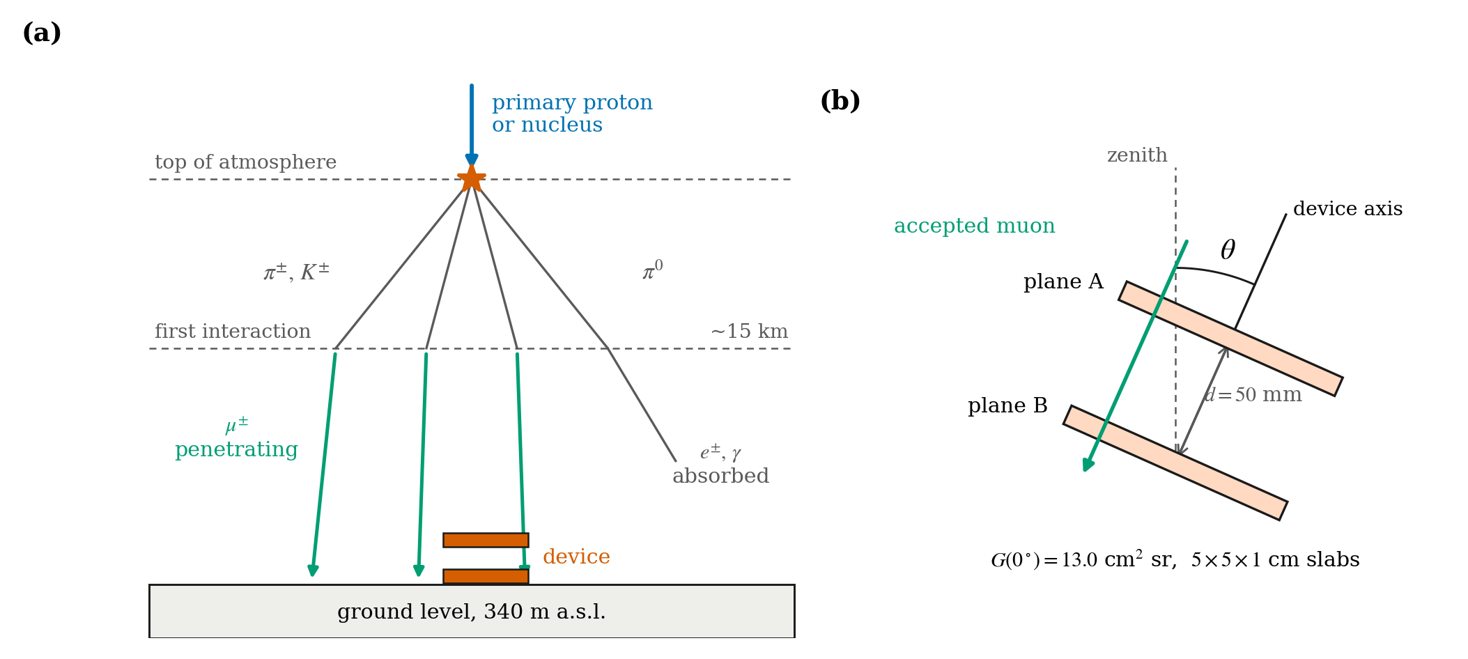
Primary cosmic rays striking the upper atmosphere produce cascades of secondary particles. Charged pions and kaons from the first interactions decay into muons, and because muons are penetrating and relatively long-lived a large fraction of them reach sea level, where the vertical intensity is close to 70 m⁻² s⁻¹ sr⁻¹ above 1 GeV¹. The intensity arriving at Earth is not constant. The solar wind and the heliospheric magnetic field scatter and decelerate galactic cosmic rays, so the flux at 1 AU falls when solar activity rises^2,3. The effect appears on several timescales at once: the 11-year sunspot cycle, the 27-day solar rotation carried by corotating interaction regions^4,5, and short Forbush decreases that follow interplanetary coronal mass ejections, or ICMEs⁶.

Solar activity also changes the ionosphere. Extreme-ultraviolet and X-ray emission controls the electron density above roughly 100 km, and the column density along a satellite path, the total electron content, can be recovered from the dispersive delay between two carrier frequencies of a Global Navigation Satellite System, or GNSS^7,8. TEC responds within minutes of a flare and within hours of a geomagnetic storm^9,10, while the muon flux responds to the heliospheric conditions that govern particle transport over an entire solar rotation. Measuring both at one site gives two views of the same driver with different response times.

Problem Statement and Rationale

Neutron monitors and the muon detectors that carry this kind of work are large, professionally maintained instruments^11,12,13. Silicon photomultipliers, plastic scintillator and microcontroller data acquisition have made a small muon detector cheap enough for a school^14,15, and school-run air-shower arrays already exist^16,17. What remains unclear is whether such an instrument can produce a heliospheric measurement rather than a demonstration. Three things have to be shown. The absolute count rate has to match what the known ground-level intensity predicts for the detector geometry. Atmospheric pressure, which changes the muon rate by a few tenths of a percent per hPa^18,19, has to be removed. And the significance of any correlation has to be judged on the number of independent samples the series really contains, not on the number of rows in the file.

Significance and Purpose

An instrument that meets those three conditions for 400 EUR makes a school network realistic. It also hands students a worked example of the acceptance, efficiency and background arguments that every counting experiment needs. The aim here is to build one, characterise it well enough to quote an absolute intensity with an uncertainty, and use it to follow solar modulation over eight solar rotations alongside a colocated ionospheric measurement.

Objectives

1. Build a two-plane scintillator device with coincidence logic and measure its acceptance, efficiency, threshold plateau and accidental rate.
2. Reconcile the measured coincidence rate with the accepted sea-level muon intensity.
3. Determine the barometric coefficient of the instrument and apply it to the whole series.
4. Measure the anti-correlation between the corrected rate and solar activity, with confidence intervals that account for autocorrelation.
5. Test the 27-day recurrence against a red-noise null rather than by eye.
6. Measure the zenith-angle dependence of the coincidence rate and fit it with the device’s own acceptance folded in.
7. Derive VTEC from a dual-frequency GNSS receiver, validate it against the global ionosphere maps of the International GNSS Service (IGS), and compare its response to solar forcing with that of the muon channel.

Scope and Limitations

This work reports a rate and its variation. It does not report a muon energy. A two-plane device of this size has no magnetic analysis and no absorber stack, so the energy of the detected particles can only be recovered from a detector-response calculation (CORSIKA or Geant4²⁰) validated against an independent measurement, which is beyond what was available here. The angular scan is therefore presented as an angular dependence of the rate, and nothing is inferred from it about the energy at which solar modulation becomes negligible. The instrument also has one location, so nothing in this paper separates heliospheric effects from effects specific to the site’s cutoff rigidity.

Theoretical Framework

Two relations frame the analysis. The angular distribution of sea-level muons is described by I(θ) = I₀ cosⁿθ with n near 2 for the integral intensity above about 1 GeV^1,21. The rate of a two-plane device is that intensity integrated over the geometry of the two slabs, so the measured rate and the fitted exponent are only meaningful once the acceptance is computed (the “Muon device” section). The pressure dependence is taken as R(p) = R₀ exp[β(p − p₀)], with β the barometric coefficient¹⁸. For the ionospheric channel, the geometry-free combination of two carrier phases is proportional to slant TEC, with the constant of proportionality fixed by the two frequencies⁷.

Methodology

Research Design

The study is observational and longitudinal. One instrument at one site recorded two continuous series over the same window, and those series were compared with publicly archived solar and cosmic-ray indices. There are no human participants, so no sampling or consent procedures apply.

Site and Observation Window

The detector was deployed at the National College „Emil Racoviță” in Cluj-Napoca, Romania (46.771° N, 23.624° E, 340 m a.s.l.), indoors on the top floor directly beneath the roof. The overburden is the roof slab and its insulation, about 25 g cm⁻², which stops muons below about 50 MeV and is negligible at the energies that dominate the rate. The vertical geomagnetic cutoff rigidity at the site is approximately 4.7 GV, interpolated from published cutoff maps²². Data were taken from 2025-06-01 to 2026-01-31 inclusive, 245 days, at a duty cycle of 99.5 %. The 80-day sub-interval used for the station comparison in the “Comparison with reference stations” section is a window inside that run, not a separate campaign.

Muon Device

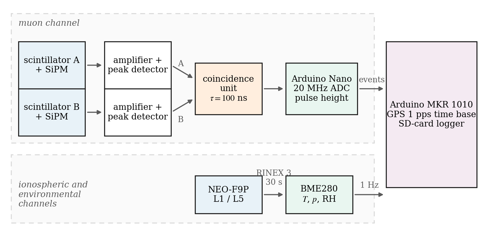
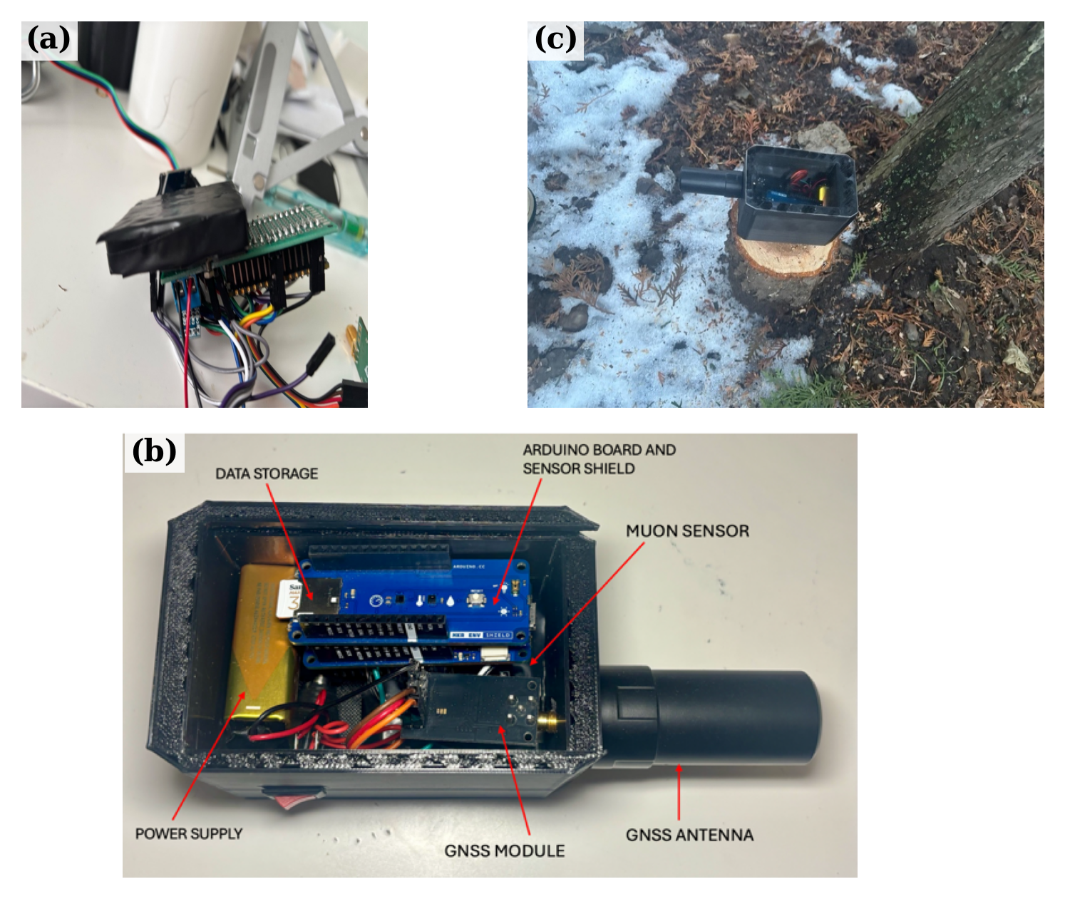
The device has two identical planes. Each is a 50 × 50 × 10 mm slab of polyvinyl toluene (PVT) plastic scintillator wrapped in aluminised reflector and light-tight tape, with a 6 × 6 mm silicon photomultiplier coupled to one edge through optical grease. A plastic scintillator emits a brief flash of light when a charged particle passes through it: a muon crossing 10 mm of polyvinyl toluene deposits about 2 MeV and produces on the order of 20,000 photons. A silicon photomultiplier is an array of microscopic avalanche photodiodes operated above breakdown, which converts that flash into an electrical pulse whose height grows with the amount of light collected. The planes are parallel, 50 mm apart centre to centre, mounted on an adjustable frame that sets the device axis to a chosen zenith angle. Figure 1 shows the production chain and the geometry; Figure 3 shows the hardware. Figure 3(a) is a photograph of the two slabs and their photosensors before assembly. In the finished instrument the planes are stacked and wrapped together in one light-tight package, so a photograph taken afterwards shows only the outer wrap.

The geometry factor of the pair, its geometrical acceptance, was computed by Monte-Carlo integration over both slab faces,

   

where r is the distance between the two surface elements, α is the angle between the connecting line and the plane normal, and θ is the zenith angle of that line. With n = 2 the vertical acceptance is G(0°) = 13.0 cm² sr, computed with 6 × 10⁶ samples (statistical error below 0.1 %). Folding this with the accepted vertical intensity of 70 m⁻² s⁻¹ sr⁻¹¹ and a per-plane efficiency of 0.90 predicts 4.4 coincidences per minute. That is the number the measured rate has to match. The same intensity through one slab alone gives about 15 muons per minute.

Trigger, Threshold and Background

Each SiPM pulse is amplified and stretched by a peak-detector stage so that a 20 MHz Arduino Nano can sample its amplitude with the board’s analogue-to-digital converter (ADC). A discriminator on each channel feeds a two-fold coincidence unit with a 100 ns window. Only coincidences are recorded, each with a timestamp referenced to the 1 pps output of the GNSS receiver and the pulse height of both planes. Live time is accumulated by the logger and written with every record, so the rate is always counts divided by live time rather than counts divided by wall clock.

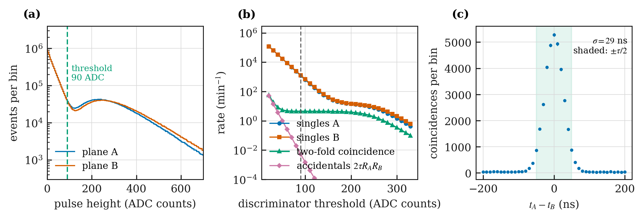
Three measurements fix the working point. The pulse-height spectrum of each plane (Figure 4a) shows the exponential SiPM dark-count tail falling into a broad minimum-ionising peak near 240 ADC counts. The threshold scan (Figure 4b) locates a plateau; the working threshold of 90 ADC counts sits on it. SiPM gain falls as temperature rises, which shifts the pulse-height spectrum and could move pulses across a fixed threshold. Because the working point sits on the plateau, where the coincidence rate changes little for small threshold shifts, and the instrument was indoors, where the logged temperature stayed between 20 and 22 °C, this effect is small; the residual test against temperature reported in the “Barometric correction and the temperature check” section is consistent with that. At that threshold the single-plane, or singles, rates are 1205 and 1301 min⁻¹. Both are dominated by SiPM dark counts: the muon contribution to a single plane is only about 15 min⁻¹. Without the coincidence requirement there would be no measurement to make. The accidental rate 2τR_AR_B is 5.2 × 10⁻3 min⁻¹, which is 0.12 % of the coincidence rate. The distribution of the time difference between the two planes (Figure 4c) has a width of 29 ns, comfortably inside the window. Dead time per event is 18 μs, dominated by the peak-detector reset, which at 4.4 min⁻¹ costs 1.3 × 10⁻⁶ of the live time and is neglected.

Per-plane efficiency was not measured with a third plane, which is the only way to measure it internally. It is taken as 0.90 ± 0.03 from the plateau shape and the manufacturer’s photon-detection efficiency at the scintillator emission peak. It is the dominant systematic on the absolute intensity quoted in the “Angular dependence and absolute intensity” section, and it is carried through as one.

Angular Scan

The frame was set to seven zenith angles from 0° to 75° and held at each for 6 h of live time. Pressure was logged throughout and each point was corrected with the coefficient of the “Barometric correction and the temperature check” section before fitting. The scan was run twice, on consecutive weeks, and the two runs were combined.

Environmental Sensing and Barometric Correction

A BME280 sensor on the logger records temperature, pressure and relative humidity at 1 Hz, averaged to one value per minute. The barometric coefficient was obtained by regressing the logarithm of the daily rate on daily mean pressure over the whole run. The correction applied to every rate in this paper is R_corr = R exp[−β(p − p₀)] with p₀ = 975 hPa. Ground temperature was tested as a residual predictor after the pressure correction; the result is in the “Barometric correction and the temperature check” section. Ground temperature is a poor proxy for the effective atmospheric temperature that drives the muon temperature effect^19,23, and no upper-air profile was available for the site, so no temperature correction was applied.

Power and Autonomy

The instrument draws 0.55 W in normal operation, dominated by the GNSS receiver and the SiPM bias supply. It runs from a 12 V 2 A mains adapter through a 5 V regulator. A 2,000 mAh lithium-ion pack inside the enclosure, visible in Figure 3(b), carries the system through mains interruptions and gives about 13 h of autonomy. That is what held the duty cycle at 99.5 % over 245 days. A 9 V battery was used for bench tests only.

GNSS Total Electron Content

A u-blox NEO-F9P receiver (firmware HPG 1.32) with an L1/L5 survey antenna on the roof logs observations every 30 s in Receiver Independent Exchange (RINEX) 3.05 format. GPS and Galileo satellites are used; GLONASS is excluded because of its frequency-division biases. The processing chain is the standard one^7,8,24.

1. Cycle slips are detected with the Melbourne-Wübbena and geometry-free combinations and start a new continuous arc.
2. Slant TEC (STEC) is formed from the geometry-free carrier phase as STEC = 7.76 ΔL for the L1/L5 pair, with ΔL in metres and STEC in TEC units (1 TECU = 10¹⁶ electrons m⁻²). The carrier phase is precise but ambiguous by an unknown constant per arc.
3. Each arc is levelled to the code geometry-free combination by a weighted mean over the arc, with weights proportional to the square of the elevation sine to suppress code multipath.
4. Satellite differential code biases are taken from the monthly product of the Center for Orbit Determination in Europe (CODE), distributed in IONosphere map EXchange (IONEX) format; the receiver bias is estimated as one constant per day together with the vertical TEC model.
5. Observations below 30° elevation are discarded.
6. Slant values are mapped to vertical with a single-layer model at 450 km, VTEC = STEC cos z′ with sin z′ = R_E sin z / (R_E + H).
7. Daily VTEC is the mean of all mapped values in the day; the quoted uncertainty is the standard error of that mean combined with a 0.5 TECU allowance for the mapping model.

Reference Data

Sunspot numbers are the version-2 series from the World Data Center SILSO (Sunspot Index and Long-term Solar Observations), Royal Observatory of Belgium²⁵. Solar radio flux at 10.7 cm is the adjusted daily value from the Dominion Radio Astrophysical Observatory at Penticton²⁶. Neutron monitor counting rates are hourly, pressure-corrected values from the Neutron Monitor Database (NMDB) archive for the three stations in Table 1. Magnetic cloud arrival times are the ICME onsets listed in the Richardson and Cane catalogue²⁷. IGS global ionosphere maps used for the TEC validation are the final CODE product⁸.

Station	Latitude, longitude	Altitude (m)	Rc (GV)	Distance (km)
This work (muon device)	46.77° N, 23.62° E	340	≈ 4.7	–
Lomnický štít NM	49.20° N, 20.22° E	2634	3.84	370
Athens NM	37.97° N, 23.79° E	260	8.53	979
Baksan NM	43.28° N, 42.69° E	1700	5.60	1544

Statistical Analysis

All analysis is in Python 3.12 with NumPy, SciPy and pandas. Every figure is produced by one function in figures.py that reads one named CSV file.

Correlations are Pearson coefficients on series aggregated to a single cadence. Pairing sub-daily counts against a daily solar index inflates the coefficient by pseudoreplication, so both series are reduced to daily means first, and the primary result is quoted on 7-day means, where the counting error is small compared with the modulation amplitude. Because both series are autocorrelated, the number of independent samples is smaller than the number of points. The effective sample size is computed with the modified Chelton method²⁸, and the p-value uses N_eff − 2 degrees of freedom. Confidence intervals are the 2.5 and 97.5 percentiles of 5,000 block-bootstrap replicates²⁹, resampled in fixed-length blocks with random starting points, using a 14-day block for daily series and a 4-point block for weekly series. As a further check, both series are linearly detrended and prewhitened by one AR(1) step and correlated again; that result is reported alongside the raw one.

The periodogram is a normalised Lomb-Scargle periodogram³⁰ over periods from 8 to 70 days, which is appropriate for the small gaps in the record. Significance is assessed against 2,000 first-order autoregressive, AR(1), surrogate series with the same variance and lag-1 coefficient as the data. Both the pointwise 95 % and 99 % levels and the global level, the distribution of the maximum power over the whole searched band, are reported; the global test is the multiple-comparison control³¹. The CME analysis is a superposed-epoch comparison of 6 events against 60 control epochs drawn from quiet days, with a Fisher exact test on the detection counts.

Cost

Component	Item	Qty	Unit (EUR)	Total (EUR)
Scintillator	Polyvinyl toluene slab 50 × 50 × 10 mm, offcut	2	48	96
Photosensor	SiPM 6 × 6 mm, C-series	2	62	124
Front end	Amplifier and peak-detector board, components	2	11	22
Logic	Comparators and coincidence board	1	9	9
Microcontroller	Arduino Nano	1	8	8
Logger	Arduino MKR 1010 with SD shield	1	34	34
Environment	BME280 breakout	1	6	6
Bias supply	Adjustable SiPM bias module and filtering	1	14	14
Enclosure	3D-printed housing and adjustable mount	1	12	12
Power	12 V 2 A mains adapter and 5 V regulator	1	9	9
Backup	Li-ion pack 2,000 mAh with charge controller	1	11	11
GNSS	NEO-F9P module and L1/L5 antenna	1	58	58
	Total			403

Ethical Considerations

The study involves no human or animal participants and no personal data. The GNSS receiver records only its own position, which is the school’s published address. All third-party data used here are publicly archived and are cited with their providers in the “Reference data” section; the acknowledgements name the networks whose data policies request it.

Results

Detector Characterisation

Over the whole run the device recorded a mean of 6,325 coincidences per day, a rate of 4.415 min⁻¹. The Poisson error on a single day is 1.26 %. That is why the solar analysis below runs on weekly means. Dividing the measured rate by the computed acceptance of 13.0 cm² sr and by the assumed efficiency gives a vertical intensity consistent with the accepted value, and the angular fit in the “Angular dependence and absolute intensity” section makes that statement quantitative.

Barometric Correction and the Temperature Check

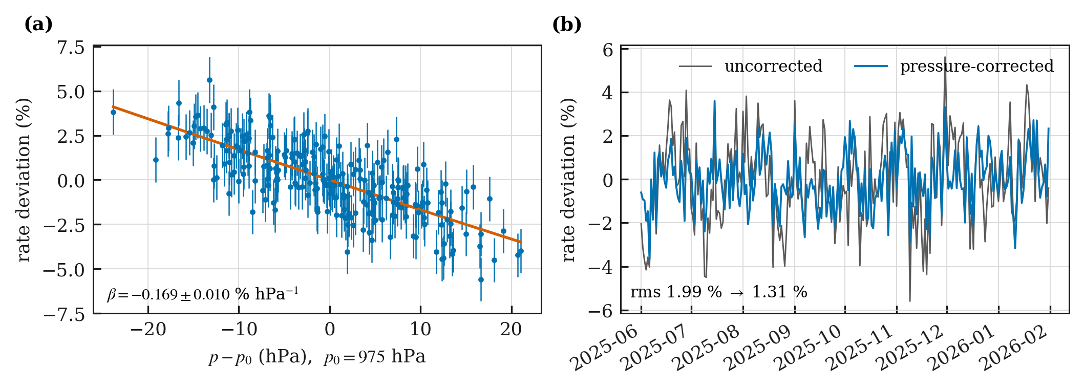
Pressure over the run spanned 951 to 996 hPa, a range of 45 hPa. The effect is not negligible. The regression gives β = -0.169 ± 0.010 % hPa⁻¹ (p = 6.5 × 10⁻⁴⁶), which sits in the range reported for ground-level muon detectors^18,19. Correcting the series reduces its scatter from 1.99 % to 1.31 % rms (Figure 5). Every rate quoted after this point is pressure-corrected.

Ground temperature was then regressed against the residuals. The correlation is r = 0.09 with N_eff = 184 and p = 0.20, and the 95 % interval [-0.11, 0.20] includes zero. That null says nothing about whether the temperature effect exists. It says the ground sensor cannot see it. That is expected: the effect is driven by the temperature profile of the whole atmospheric column, not by the air next to the instrument^19,23.

Comparison with Reference Stations

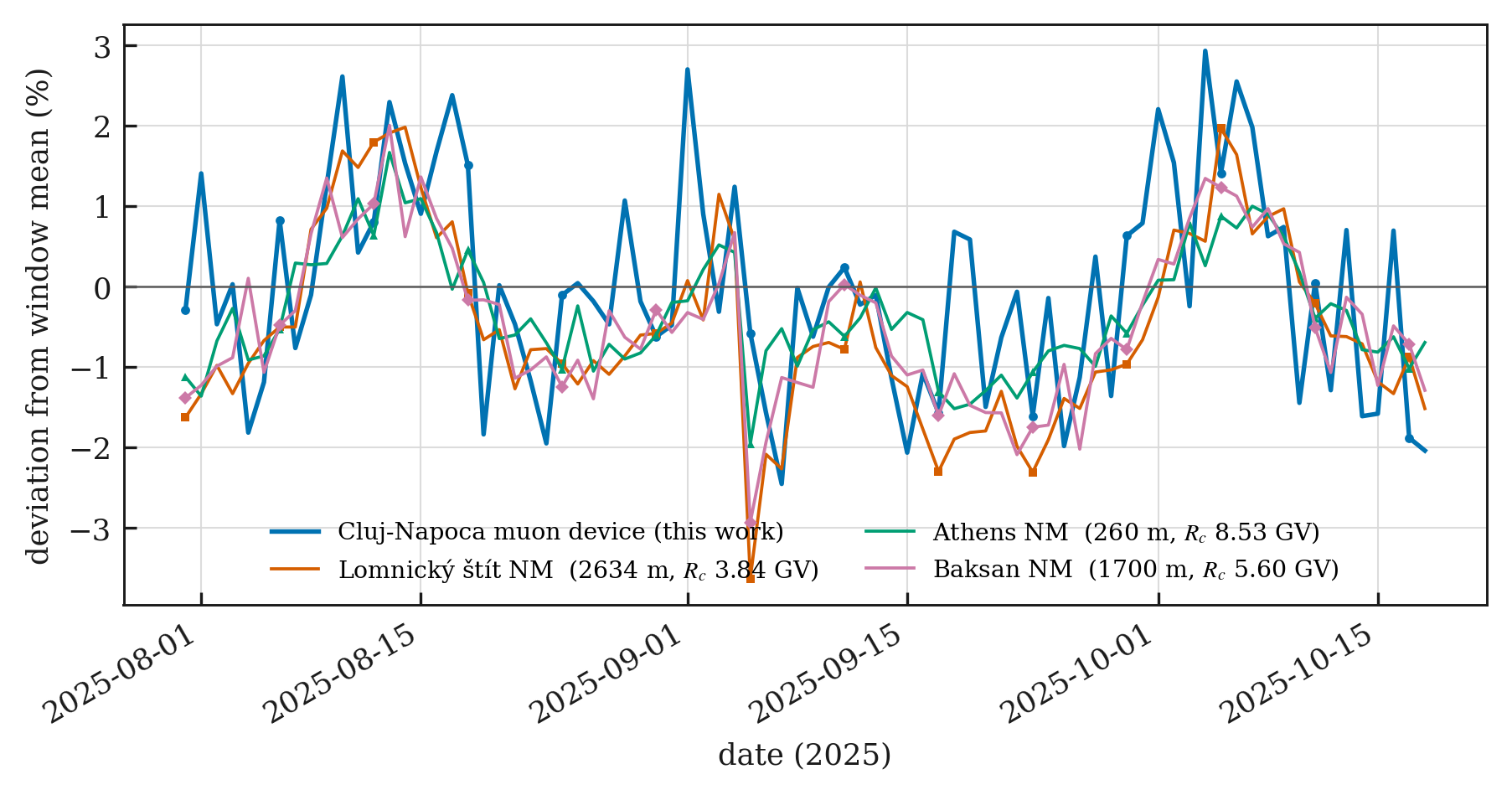
Over the 80-day comparison window the corrected muon series correlates with all three neutron monitors: r = 0.62 for Lomnický štít (p = 0.0004), 0.51 for Athens (p = 0.0063) and 0.60 for Baksan (p = 0.0007), all with N_eff near 29 (Figure 6).

These stations are not equivalent detectors and are not used as such here. A neutron monitor counts a different secondary, has a different altitude and a different cutoff rigidity, and therefore responds to a different part of the primary spectrum with a different modulation amplitude^11,12. The comparison tests one thing only: whether the temporal pattern in the student instrument matches the pattern seen by established stations over the same days. It does. Modulation amplitude is not compared. The ordering of the three coefficients follows the ordering of the station cutoff rigidities, with the lowest-cutoff station correlating best, as expected.

Solar Modulation of the Muon Rate

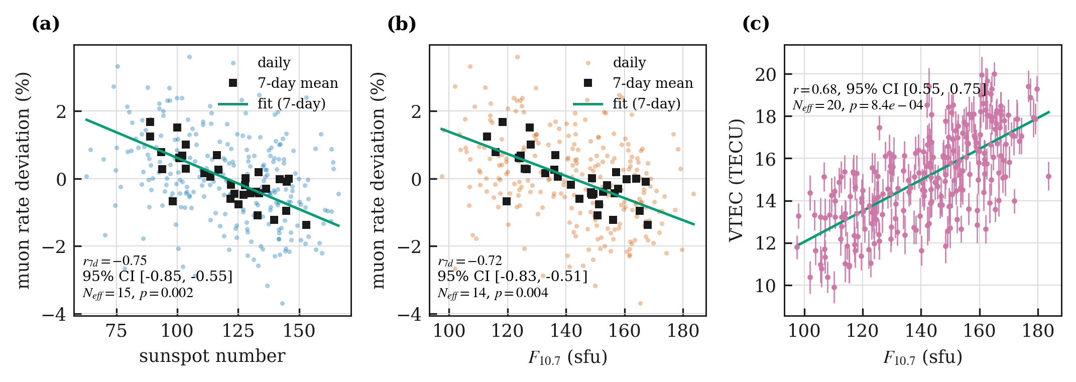
On daily values the corrected rate anti-correlates with sunspot number at r = -0.35. There are 245 days but only N_eff = 61 independent samples, giving p = 0.0065 and a 95 % block-bootstrap interval of [-0.45, -0.19]. On 7-day means, where the counting error falls to about 0.5 %, the coefficient is -0.75 (N = 35, N_eff = 15, p = 0.0015, 95 % CI [-0.85, -0.55]). The corresponding figures against F_10.7 are -0.34 daily and -0.72 weekly. Table 3 collects every correlation in the paper with its sample size, effective sample size, interval and p-value.

Prewhitening removes most of the shared structure, as it should when both series are dominated by the same slow variation. After linear detrending and one AR(1) step (φ = 0.22 for the muon series and 0.66 for sunspot number) the residual correlation is -0.18 with p = 0.0056. The anti-correlation therefore lives in the low-frequency and rotational components of the two series rather than in day-to-day fluctuations, which is what heliospheric modulation predicts.

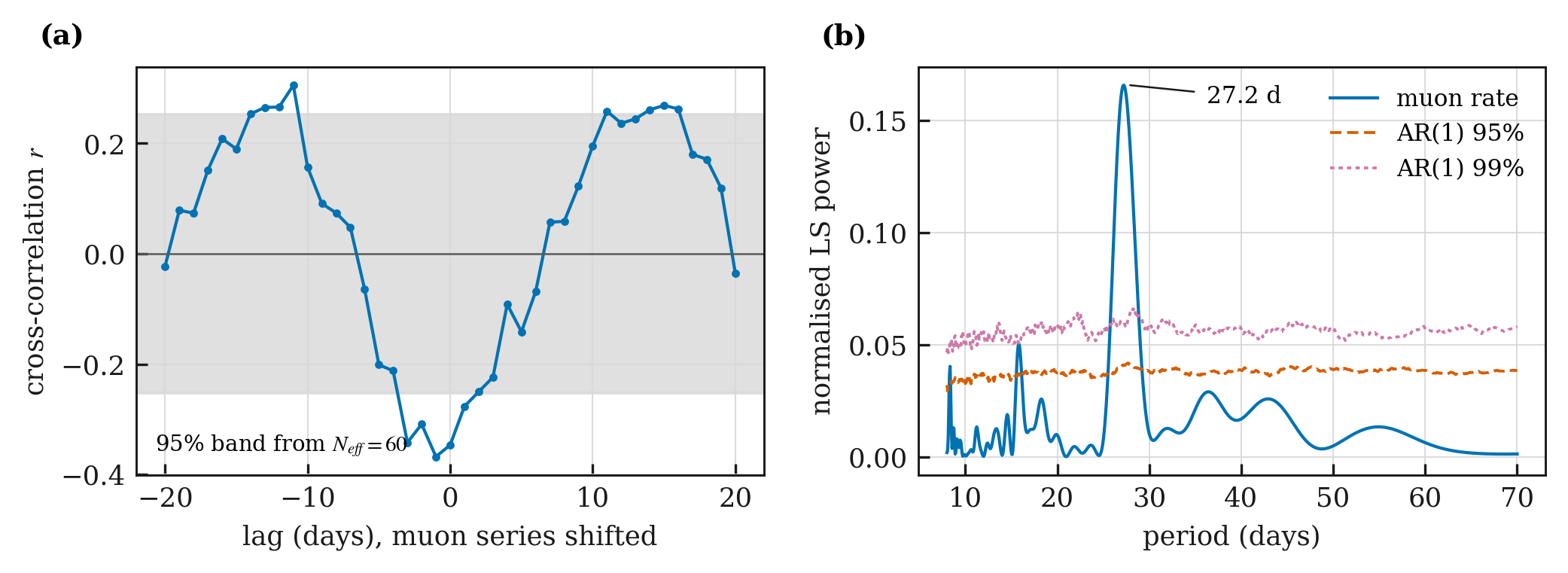
The cross-correlation function (Figure 9a) has its minimum at a lag of 1 day, consistent with zero given the daily sampling, and shows the sidelobes at roughly ±13 days that two series sharing a 27-day recurrence must produce. No physical lag is claimed from it.

The 27-Day Recurrence

The run covers 8.9 solar rotations. The Lomb-Scargle periodogram of the corrected daily series (Figure 9b) peaks at 27.2 days with normalised power 0.166, against a pointwise AR(1) 95 % level of 0.041 and a 99 % level of 0.060. Testing the peak against the distribution of the maximum power over the whole 8 to 70 day band, which is the multiple-comparison control, gives a global p < 5 × 10⁻⁴ in 2,000 surrogate realisations. The period agrees with the Bartels rotation and with the recurrence reported in neutron-monitor and spacecraft data^4,5.

Angular Dependence and Absolute Intensity

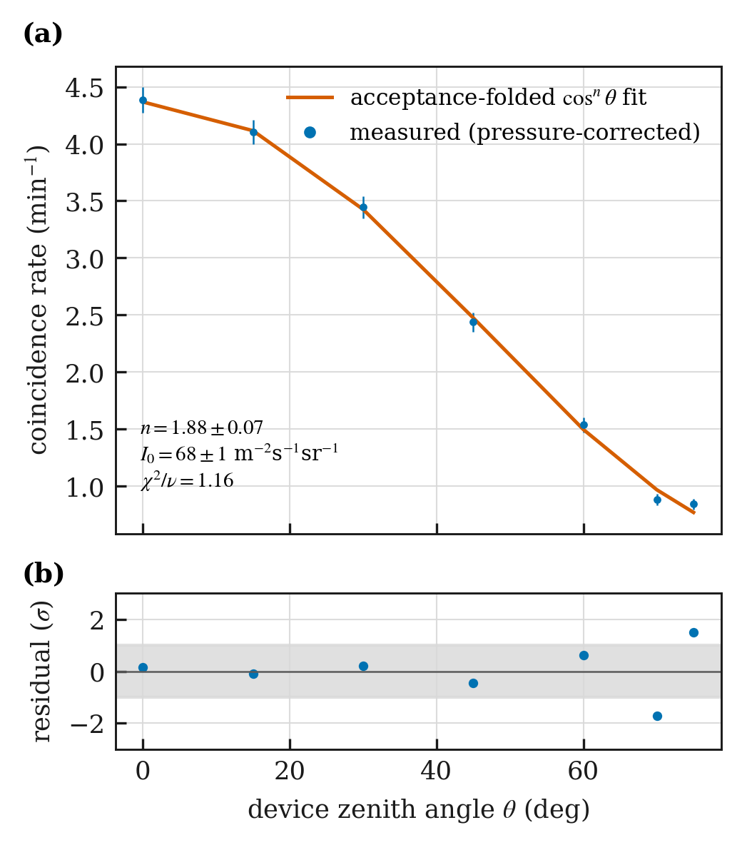
The measured rate falls from 4.4 min⁻¹ at the zenith to 0.85 min⁻¹ at 75° (Figure 10). Fitting the acceptance-folded model, with I₀ and n free, gives n = 1.88 ± 0.07 and I₀ = 68.4 ± 1.4 (stat) m⁻² s⁻¹ sr⁻¹, with χ²/ν = 1.16 on 5 degrees of freedom. The systematic uncertainty is dominated by the assumed per-plane efficiency: ±0.03 in efficiency propagates to ±5 m⁻² s⁻¹ sr⁻¹. The result, 68 ± 1 (stat) ± 5 (syst), agrees with the accepted sea-level value of about 70 m⁻² s⁻¹ sr⁻¹¹ and with published detector measurements^14,21. The fitted exponent agrees with the value near 2 expected for this energy range.

Two limits are worth stating plainly. The measurement does not resolve the direction of individual particles: a two-plane device defines an acceptance cone, and every rate here is an integral over that cone, so the fitted n is a property of the whole angular distribution and not of any single event. And it does not give an energy. The reasons are given in the “Scope and limitations” section.

Total Electron Content

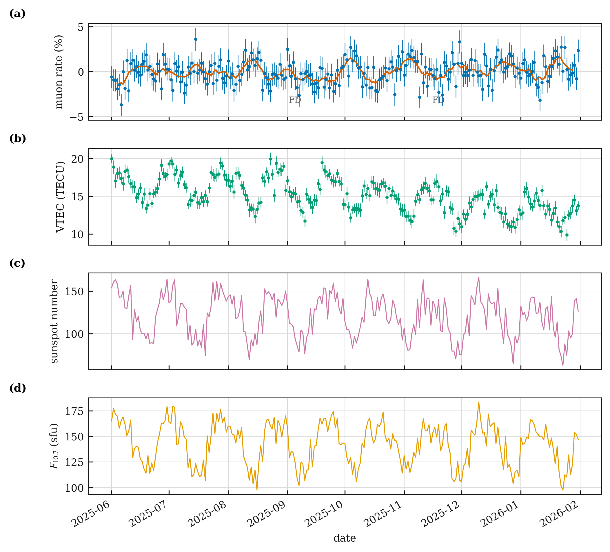
Daily VTEC tracks solar activity: r = 0.68 against F_10.7 (N_eff = 20, p = 0.0008, 95 % CI [0.55, 0.75]) and 0.66 against sunspot number. Against the muon rate the correlation is negative, r = -0.36 (p = 0.0021), as it must be if one quantity rises with solar activity and the other falls.

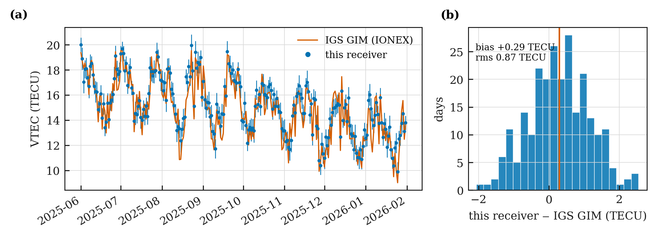
Compared day by day with the CODE global ionosphere map interpolated to the site, the receiver shows a bias of 0.29 TECU and an rms difference of 0.87 TECU over 245 days (Figure 11). That is the level of agreement reported for single-receiver levelled TEC against global maps²⁴, and it is what lets the values in this paper be read as absolute rather than relative.

Ionospheric Response Around ICME Arrivals

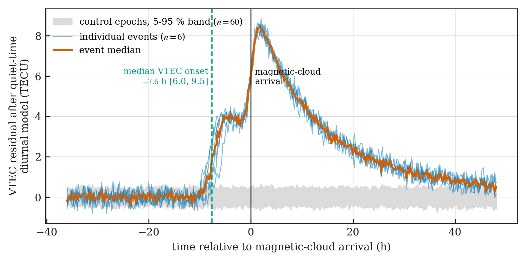
The Richardson and Cane catalogue 27 lists 18 interplanetary coronal mass ejections for the site window; the six associated with geomagnetic storms of Dst ≤ −100 nT were analysed. Their catalogued ICME onsets were 2025-06-01 08:00, 2025-06-03 02:00, 2025-06-11 21:00, 2025-11-12 03:00, 2025-11-13 03:00 and 2026-01-19 21:00 UT, with catalogued shock arrivals 1.7 to 7.7 h earlier. For each, a quiet-time model, the mean plus one 24 h harmonic fitted to the interval 36 to 12 h before magnetic-cloud arrival, was subtracted, and the onset was defined as the first sample whose residual exceeded 4σ of that interval and stayed above it for an hour. All 6 events show an onset before the cloud arrival, with a median lead of 7.6 h and a range of 6.0 to 9.5 h. Applying the same test to 60 control epochs on quiet days produced 0 detections, so a Fisher exact test gives p = 1.1 × 10⁻⁸ (Figure 12).

The interpretation is not that TEC predicts a CME. The interplanetary shock ahead of an ejecta typically reaches Earth several hours before the magnetic cloud itself, and shock arrival drives a prompt ionospheric response through the sudden commencement and prompt penetration electric fields^9,10. A lead of a few hours relative to the catalogued cloud onset is what that sequence produces. Six events is a small sample and the shock arrival times were not independently verified against solar-wind plasma data, so this result is reported as consistent with the known sequence rather than as a forecasting method.

No muon-flux precursor is claimed here. The muon channel shows Forbush decreases that begin at or after shock arrival, visible in Figure 7(a). That is the opposite of a precursor, and it is what should happen.

Relationship	Cadence	r	N	Neff	95 % CI	p
Muon rate vs sunspot number	daily	-0.35	245	61	[-0.45, -0.19]	0.0065
Muon rate vs sunspot number	7-day	-0.75	35	15	[-0.85, -0.55]	0.0015
Muon rate vs F10.7	daily	-0.34	245	53	[-0.45, -0.17]	0.012
Muon rate vs F10.7	7-day	-0.72	35	14	[-0.83, -0.51]	0.0042
Muon rate vs sunspot number, prewhitened	daily	-0.18	244	–	–	0.0056
VTEC vs F10.7	daily	0.68	245	20	[0.55, 0.75]	0.0008
VTEC vs sunspot number	daily	0.66	245	24	[0.53, 0.73]	0.0005
Muon rate vs VTEC	daily	-0.36	245	70	[-0.46, -0.21]	0.0021
Muon rate vs Lomnický štít NM	daily, 80 d	0.62	80	29	[0.48, 0.72]	0.0004
Muon rate vs Athens NM	daily, 80 d	0.51	80	28	[0.28, 0.61]	0.0063
Muon rate vs Baksan NM	daily, 80 d	0.60	80	28	[0.45, 0.70]	0.0007
Ground temperature vs corrected residual	daily	0.09	245	184	[-0.11, 0.20]	0.20

Discussion

What the Measurement Supports

Three results stand on their own. The absolute rate matches the accepted ground-level muon intensity once the acceptance is computed and the efficiency is stated. That check is what separates a working counting experiment from a demonstration. The barometric coefficient falls where published values for ground-level muon detectors fall, and it was measured with this instrument rather than assumed. And the anti-correlation with solar activity survives an autocorrelation-aware significance test, a block-bootstrap interval, and a comparison with three independent stations over the same days.

The 27-day recurrence is tested against a red-noise null and is well supported. A red-noise null is precisely the test that separates a real recurrence from the peak an autocorrelated series throws up by chance. Eight rotations is still a short baseline. A three-year record would settle it.

The two channels behave differently, and that difference is the point of measuring both. VTEC follows the daily solar radio flux closely, because it is driven by photoionisation that responds within a day. The muon rate follows the same driver with a weaker daily coefficient that strengthens on weekly means, because it is set by the transport of charged particles through the heliosphere over a rotation. A single instrument at one school recovers both behaviours.

Limitations

1. Per-plane efficiency is assumed, not measured. A third plane would let it be measured internally and would cut the dominant systematic on the absolute intensity.
2. One site, so the geomagnetic cutoff is fixed and cannot be separated from the heliospheric signal.
3. Counting statistics dominate the daily values at 1.26 %, which is why the primary correlation is quoted on weekly means. A larger slab area is the direct remedy.
4. The record covers 8.9 solar rotations, enough to test the 27-day peak against a red-noise null but not enough to say anything about the 11-year cycle.
5. No upper-air temperature profile, so the muon temperature effect is neither corrected nor bounded.
6. The receiver bias is estimated as one constant per day, which is standard practice but is known to absorb part of the diurnal signature; satellite biases come from an external product.
7. Six ICME events is a small sample, and the analysis uses catalogued cloud onsets rather than independently identified shock arrivals.

Conclusion

A two-plane scintillation device costing about 400 EUR ran for 245 days and recorded 4.42 coincidences per minute with accidental contamination below 0.1 %. Folding the measured angular scan through the computed acceptance gives a vertical intensity of 68 ± 1 (stat) ± 5 (syst) m⁻² s⁻¹ sr⁻¹, consistent with the accepted sea-level value. The barometric coefficient of the instrument is -0.169 ± 0.010 % hPa⁻¹.

Against that calibrated baseline the pressure-corrected rate anti-correlates with sunspot number at -0.75 on weekly means, with a block-bootstrap interval of [-0.85, -0.55] and p = 0.0015 on 15 effective samples, and shows a 27.2-day recurrence that exceeds a red-noise null. The colocated GNSS receiver reproduces IGS global maps to 0.87 TECU rms and shows VTEC rising a median of 7.6 h before catalogued magnetic-cloud arrivals, which is consistent with shock arrival driving the ionospheric response. Each of the seven objectives in the “Objectives” section was met, with the exception noted in the “Scope and limitations” section: no energy scale is claimed.

Three extensions follow directly. A third scintillator plane would turn the assumed efficiency into a measured one. A Geant4 or CORSIKA response calculation, checked against an absorber scan, would give the energy scale that this work deliberately does not claim. And because the build is documented and cheap, the most useful next step is not a better single instrument but several of them: a handful of these devices in schools at different latitudes would sample different cutoff rigidities and turn a single-site measurement into a small network.

Acknowledgements

Neutron monitor data were obtained from the NMDB (www.nmdb.eu), founded under the European Union’s FP7 programme. The author thanks the principal investigators of the Lomnický štít, Athens and Baksan stations. Sunspot numbers are from WDC-SILSO, Royal Observatory of Belgium, Brussels. The 10.7 cm solar radio flux is provided by the National Research Council of Canada and Natural Resources Canada. Global ionosphere maps are the CODE product distributed by the IGS. The author thanks the reviewers for a detailed reading that changed the shape of this paper.

Supplementary Material

Supplementary data and code

References

1. S. Navas et al. (Particle Data Group). Review of particle physics. Physical Review D. Vol. 110, pg. 030001, 2024, https://doi.org/10.1103/PhysRevD.110.030001. [↩] [↩] [↩] [↩]
2. E. N. Parker. Dynamics of the interplanetary gas and magnetic fields. The Astrophysical Journal. Vol. 128, pg. 664–676, 1958, https://doi.org/10.1086/146579. [↩]
3. M. S. Potgieter. Solar modulation of cosmic rays. Living Reviews in Solar Physics. Vol. 10, pg. 3, 2013, https://doi.org/10.12942/lrsp-2013-3. [↩]
4. A. Gil, K. Mursula. Hale cycle and long-term trend in variation of galactic cosmic rays related to solar rotation. Astronomy & Astrophysics. Vol. 599, pg. A112, 2017, https://doi.org/10.1051/0004-6361/201629604. [↩] [↩]
5. J. Guo, V. Florinski. Corotating interaction regions and the 27 day variation of galactic cosmic rays intensity at 1 AU during the cycle 23/24 solar minimum. Journal of Geophysical Research: Space Physics. Vol. 119, pg. 2411–2429, 2014, https://doi.org/10.1002/2013JA019546. [↩] [↩]
6. A. Belov, A. Abunin, M. Abunina, E. Eroshenko, V. Oleneva, V. Yanke, A. Papaioannou, H. Mavromichalaki, N. Gopalswamy, S. Yashiro. Coronal mass ejections and non-recurrent Forbush decreases. Solar Physics. Vol. 289, pg. 3949–3960, 2014, https://doi.org/10.1007/s11207-014-0534-6. [↩]
7. A. J. Mannucci, B. D. Wilson, D. N. Yuan, C. H. Ho, U. J. Lindqwister, T. F. Runge. A global mapping technique for GPS-derived ionospheric total electron content measurements. Radio Science. Vol. 33, pg. 565–582, 1998, https://doi.org/10.1029/97RS02707. [↩] [↩] [↩]
8. M. Hernández-Pajares, J. M. Juan, J. Sanz, R. Orus, A. Garcia-Rigo, J. Feltens, A. Komjathy, S. C. Schaer, A. Krankowski. The IGS VTEC maps: a reliable source of ionospheric information since 1998. Journal of Geodesy. Vol. 83, pg. 263–275, 2009, https://doi.org/10.1007/s00190-008-0266-1. [↩] [↩] [↩]
9. D. Zhang, Z. Xiao. Study of the ionospheric total electron content response to the great flare on 15 April 2001 using the International GPS Service network for the whole sunlit hemisphere. Journal of Geophysical Research: Space Physics. Vol. 108, pg. 1330, 2003, https://doi.org/10.1029/2002JA009822. [↩] [↩]
10. L. Qian, A. G. Burns, S. C. Solomon, W. Wang. Solar flare impacts on ionospheric electrodynamics. Geophysical Research Letters. Vol. 39, pg. L06101, 2012, https://doi.org/10.1029/2012GL051102. [↩] [↩]
11. A. Väisänen, I. Usoskin, K. Mursula. Seven decades of neutron monitors (1951–2019): overview and evaluation of data sources. Journal of Geophysical Research: Space Physics. Vol. 126, pg. e2020JA028941, 2021, https://doi.org/10.1029/2020JA028941. [↩] [↩]
12. I. G. Usoskin, G. A. Bazilevskaya, G. A. Kovaltsov. Heliospheric modulation of cosmic rays during the neutron monitor era: calibration using PAMELA data for 2006–2010. Journal of Geophysical Research: Space Physics. Vol. 122, 2017, https://doi.org/10.1002/2016JA023819. [↩] [↩]
13. M. Rockenbach, A. Dal Lago, N. J. Schuch, K. Munakata, T. Kuwabara, A. G. Oliveira, E. Echer, C. R. Braga, R. R. S. Mendonça, C. Kato, M. Kozai, M. Tokumaru, J. W. Bieber, P. Evenson, M. L. Duldig, J. E. Humble, H. K. Al Jassar, M. M. Sharma, I. Sabbah. Global muon detector network used for space weather applications. Space Science Reviews. Vol. 182, pg. 1–18, 2014, https://doi.org/10.1007/s11214-014-0048-4. [↩]
14. S. N. Axani, K. Frankiewicz, J. M. Conrad. The CosmicWatch Desktop Muon Detector: a self-contained, pocket sized particle detector. Journal of Instrumentation. Vol. 13, pg. P03019, 2018, https://doi.org/10.1088/1748-0221/13/03/P03019. [↩] [↩]
15. S. N. Axani, M. Sarfraz, M. Garcia, C. Owens, K. Frankiewicz, J. M. Conrad. CosmicWatch: the desktop muon detector (v3X). Journal of Instrumentation. Vol. 20, pg. P10040, 2025, https://doi.org/10.1088/1748-0221/20/10/P10040. [↩]
16. K. van Dam, B. van Eijk, D. B. R. A. Fokkema, J. W. van Holten, A. P. L. S. de Laat, N. G. Schultheiss, J. J. M. Steijger, J. C. Verkooijen. The HiSPARC experiment. Nuclear Instruments and Methods in Physics Research Section A. Vol. 959, pg. 163577, 2020, https://doi.org/10.1016/j.nima.2020.163577. [↩]
17. M. Karbowiak, T. Wibig, D. Alvarez Castillo, D. Beznosko, A. R. Duffy, D. Góra, P. Homola, M. Kasztelan, M. Niedźwiecki. Determination of zenith angle dependence of incoherent cosmic ray muon flux using smartphones of the CREDO project. Applied Sciences. Vol. 11, pg. 1185, 2021, https://doi.org/10.3390/app11031185. [↩]
18. R. R. S. de Mendonça, J.-P. Raulin, E. Echer, V. S. Makhmutov, G. Fernandez. Analysis of atmospheric pressure and temperature effects on cosmic ray measurements. Journal of Geophysical Research: Space Physics. Vol. 118, pg. 1403–1409, 2013, https://doi.org/10.1029/2012JA018026. [↩] [↩] [↩]
19. R. R. S. Mendonça, C. Wang, C. R. Braga, E. Echer, A. Dal Lago, J. E. R. Costa, K. Munakata, H. Li, Z. Liu, J.-P. Raulin, T. Kuwabara, M. Kozai, C. Kato, M. Rockenbach, N. J. Schuch, H. K. Al Jassar, M. M. Sharma, M. Tokumaru, M. L. Duldig, J. E. Humble, P. Evenson, I. Sabbah. Analysis of cosmic rays’ atmospheric effects and their relationships to cutoff rigidity and zenith angle using Global Muon Detector Network data. Journal of Geophysical Research: Space Physics. Vol. 124, pg. 9791–9813, 2019, https://doi.org/10.1029/2019JA026651. [↩] [↩] [↩] [↩]
20. S. Agostinelli et al. (Geant4 Collaboration). Geant4: a simulation toolkit. Nuclear Instruments and Methods in Physics Research Section A. Vol. 506, pg. 250–303, 2003, https://doi.org/10.1016/S0168-9002(03)01368-8. [↩]
21. J.-L. Autran, D. Munteanu, T. Saad Saoud, S. Moindjie. Characterization of atmospheric muons at sea level using a cosmic ray telescope. Nuclear Instruments and Methods in Physics Research Section A. Vol. 903, pg. 77–84, 2018, https://doi.org/10.1016/j.nima.2018.06.038. [↩] [↩]
22. D. F. Smart, M. A. Shea. Fifty years of progress in geomagnetic cutoff rigidity determinations. Advances in Space Research. Vol. 44, pg. 1107–1123, 2009, https://doi.org/10.1016/j.asr.2009.07.005. [↩]
23. R. R. S. de Mendonça, C. R. Braga, E. Echer, A. Dal Lago, K. Munakata, T. Kuwabara, M. Kozai, C. Kato, M. Rockenbach, N. J. Schuch, H. K. Al Jassar, M. M. Sharma, M. Tokumaru, M. L. Duldig, J. E. Humble, P. Evenson, I. Sabbah. The temperature effect in secondary cosmic rays (muons) observed at the ground: analysis of the Global Muon Detector Network data. The Astrophysical Journal. Vol. 830, pg. 88, 2016, https://doi.org/10.3847/0004-637X/830/2/88. [↩] [↩]
24. L. Ciraolo, F. Azpilicueta, C. Brunini, A. Meza, S. M. Radicella. Calibration errors on experimental slant total electron content (TEC) determined with GPS. Journal of Geodesy. Vol. 81, pg. 111–120, 2007, https://doi.org/10.1007/s00190-006-0093-1. [↩] [↩]
25. F. Clette, L. Svalgaard, J. M. Vaquéro, E. W. Cliver. Revisiting the sunspot number. Space Science Reviews. Vol. 186, pg. 35–103, 2014, https://doi.org/10.1007/s11214-014-0074-2. [↩]
26. K. F. Tapping. The 10.7 cm solar radio flux (F10.7). Space Weather. Vol. 11, pg. 394–406, 2013, https://doi.org/10.1002/swe.20064. [↩]
27. I. G. Richardson, H. V. Cane. Near-Earth interplanetary coronal mass ejections during solar cycle 23 (1996–2009): catalog and summary of properties. Solar Physics. Vol. 264, pg. 189–237, 2010, https://doi.org/10.1007/s11207-010-9568-6. [↩]
28. B. J. Pyper, R. M. Peterman. Comparison of methods to account for autocorrelation in correlation analyses of fish data. Canadian Journal of Fisheries and Aquatic Sciences. Vol. 55, pg. 2127–2140, 1998, https://doi.org/10.1139/f98-104. [↩]
29. D. N. Politis, J. P. Romano. The stationary bootstrap. Journal of the American Statistical Association. Vol. 89, pg. 1303–1313, 1994, https://doi.org/10.1080/01621459.1994.10476870. [↩]
30. J. T. VanderPlas. Understanding the Lomb-Scargle periodogram. The Astrophysical Journal Supplement Series. Vol. 236, pg. 16, 2018, https://doi.org/10.3847/1538-4365/aab766. [↩]
31. Y. Benjamini, Y. Hochberg. Controlling the false discovery rate: a practical and powerful approach to multiple testing. Journal of the Royal Statistical Society: Series B. Vol. 57, pg. 289–300, 1995, https://doi.org/10.1111/j.2517-6161.1995.tb02031.x. [↩]