

Abstract
Small bakeries have to decide how much bread they will make in discrete batch units based on short and irregular sales histories. Also, point-of-sale (POS) logs have a clear limitation. After a bakery sells all the bread it made, we cannot track how many customers actually tried to buy later. Only paid sales are recorded. In this research, we evaluated RSB Forecaster, a decision-support system which helps them decide the amount of bread to make. This system uses Median-14, a model that takes the median of the last 14 observed open-day records and adjusts it by day of the week. To recommend final batch counts, this system combines the Median-14 prediction value with three factors: proxy batch sizes fixed from past POS records, uncertainty intervals calculated from prior-fold errors, and a rule-based review gate that picks items for a person to check. When we evaluated Store A, for 182 days of that data we predicted the next-day amount of bread sold by moving the forecast date forward one day at a time. Here, we only used two factors from outside: day of the week and holidays. To prevent data leakage, we excluded all information that we cannot know on the forecast day, such as target-day actual weather, closed days guessed from future POS sales, and full-period metadata, and we did not use prediction errors (residuals) from the same evaluation fold. Across all 4,810 date-SKU rows targeted for evaluation, the mean absolute error (MAE) of the prediction value was 1.87 units and the weighted mean absolute percentage error (wMAPE) was 60.09%. The recommended amount of batches matched the sales-based proxy batch count exactly on 57.90% of rows, and fell within 1 batch on 90.44% of rows. The 80% uncertainty intervals built from prior-fold residuals covered actual sales on 82.31% of the 4,782 eligible rows. The review gate classified 63.11% of eligible rows as ‘human review’. Auto-passed rows had better within-1-batch accuracy than flagged rows (95.58% vs. 87.44%). The reason why auto-passed rows had better accuracy is that they had more rows with a zero rounded proxy-batch target, which is easy to predict. Also, we compared Median-14 one-to-one with 20 different machine learning regression models on the same rows. From that result, Median-14 had no statistically significant difference from Huber regression and LinearSVR, and performed better than the other 18 models. The same tendency appeared in Store B, which had a 1,422-row fixed-cutoff stress test. While no rolling-median window length won first place for every test metric, the attempt to adjust for stockouts using rules based only on POS data actually dropped the accuracy of the prediction. Because our dataset does not have records of actual production, inventory, sell-out times, waste, or manager actions, this evaluation is limited to observed sales and simulations on past data. The main contribution of this study is to provide a reproducible way to audit next-day batch production recommendations while controlling data leakage.
Keywords: intermittent demand, observed sales, perishable retail, rolling-origin evaluation, interpretable forecasting, selective review, data leakage
Introduction
Small bakeries, when they make the bread, simultaneously have three same issues that usually researchers deal with as different factors of the problem.
First of all, only sales volume that is actually done with payment is recorded in POS. So if they sell all of the bread early, even if the consumer wants to buy, it does not appear in the statistics, it is completely different from the day when actually no one buys the bread1,2,3.
Also each bread usually has so much different amount that is actually bought from customers. Since days with no bread sold in the dataset break the normal average calculation, past studies separate the intervals at which bread is sold and amount of bread that is sold at one time and calculate4,5,6.
Additionally, production of the bread is segmented by the number of batches or by oven tray units(batches).
Also, it is a big problem that there is only a little information available to predict the amount of bread when they actually have to decide. It is easy to use the weather that will be observed tomorrow and the entire statistics prediction that includes every dataset including the day that needs to be predicted, but getting that data is impossible when they have to decide. This future information, called data leakage, allows the model to perform well but they actually cheated on the test7,8,9,10. So to fairly compare with all of them, we have to only use the information that is available for them, and make the comparison head to head, excluding rows with missing sales records.
Because of the three conditions, this changes the evaluation perspective. The big prediction competition results indicate that we should not believe that complex algorithms out compete in every competition11. Also, previous studies rigorously distinguish the predicted amount that customers buy and decisions that real stores make because they need current storage and rule of the stores that they cannot know from POS data12,13. Specifically, standard error metrics like MAE or RMSE fail to adequately capture critical factors: the thresholds for rounding when deciding how many batches to bake, the constraints of a short shelf life, and the asymmetry in the costs incurred when there is a shortage versus a surplus of bread14,15. For example, even though the prediction got 1 or 2 wrong, if it goes beyond the rounding boundary the actual batches change. In the opposite way, even though the exact number is significantly wrong, the batches it recommends won’t change.
So tools that help bakeries produce and predict the breads should have prediction models that people can see and understand the process, certain rules to change predicted numbers to real batches to make, capability to pick dangerous cases, and review mechanisms that are evaluated based on their actual classification performance.
The research that people do when the prediction is not confident emphasizes the relationship between the volume of automated processing and the risk of errors16,17. Bad explanations might lead people to be too credulous of the prediction18,19.
But when every single decision is important and a simple model can outperform, it is better to use a transparent model than black box model that requires explanation later20.
So that is why we make and evaluate RSB Forecasters based on Median-14 which is really simple and transparent. This model combines data organization based on the point in time of a decision, rounding of estimated batch quantities, forecast ranges derived from historical errors, and review gates based on rules.
There are two different standards that define the scope of the research. One of them is that the review gate was evaluated through simulations run on historical data. In other words, the simulation focused on the difference between items flagged for human review and those that passed automatically, also the percentage of total tasks requiring human intervention. (Because the system was not tested by actual managers, we did not evaluate how much we change it, how much we believe it, and how much time decreases and sales increase.) Another thing is that the algorithm only used sales volume recorded on the POS to predict and score it. Since the data does not have any actual quantity prepared, inventory levels, times when items went out of stock, or the amount of waste, the model cannot estimate latent demand, actual waste, or calculation for money.
Under this standard we checked 4 of them: how much will it be changed if we change moving median period, day-of-week adjustment, out-of-stock adjustment rules, and rounding method, and how prediction range and review gate for historical errors do well on classifying dangerous days. Additionally, we evaluated whether this simple model could compete against 20 pre-selected machine learning models when tested on the same dataset. Finally, we evaluate the accuracy of the “Median-14” approach in making next-day (D+1) forecasts, a process that excludes data such as future weather, and future sales-based store closure information, while making sure that there is no data leakage.
Methods
It runs in four steps, starting from collecting only the data we can use up to the decision day, moving to our core prediction model Median-14, changing the prediction number into an integer batch count with a prediction range, and finally using a review gate that decides if it will pass each recommendation automatically or send it to a person.
Study design and data
We only scored every prediction when that date and bread actually had a sales record of 0 or more, and in the log we separately wrote down if there was a record and how many were missing. In Store A, we took out 2 cases where the POS wrongly recorded minus sales volume(-175 and -20 on October 13, 2023) from both training and evaluation. Also, in the past training data, we saw the day when the whole store’s sales volume was 0 as a closed day and took it out, but if we use this on the day we have to predict, it becomes cheating by looking at future sales in advance to guess the closed day, so during the evaluation period we did not use this rule and predicted every day including holidays.
We put the data together by date and bread number(SKU) and made it into a daily table. The selling period for each bread starts from the first day the log records a sale, and if the record stays empty for more than one day, we saw it as a new period starting. Inside that period, we kept the day with a 0 record as real 0 sales, but when we evaluated, we took out the day that had no record at all as ‘no record’ and never forced a 0 into it.
The Store A data we used has 25,562 records of 53 SKUs from January 1, 2023 to December 31, 2025, and the sub-data Store B has 11,354 records of 42 SKUs from January 1, 2025 to February 28, 2026. This includes the date, bread number, name, category, and daily sales volume, and a separate date file has weekends, holidays, and weather. But Store A only measured the weather after the day passed and Store B used fake weather data, so since both of them are not the ‘weather forecast’ of that morning, we did not use the weather information of the day to predict at all to stop future data leakage.
Outcome definition and identifiability
So all training and scoring in this study only target the actual POS sales volume ( ) that the log records as 0 or more. When we call the production amount that the system recommends
 ,
 means the ‘certain shortage’ where the system recommended less than what actually sold, and
 means the ‘potential leftover’ where it recommended more than what sold (of course, the bread might have sold out early, so this leftover number does not mean the actual amount of bread that the store threw away).
Let’s call the POS record of bread  sold on date
 as , and the real demand that customers actually wanted to buy when there was no sell-out as
 . In a POS environment that has no records of how much bread they baked, hourly inventory, sell-out time, if customers switched to another bread, or how much they threw away, we have no way to know the real demand . The only thing we can say for sure from the data is one formula (
 ), which says the amount sold is 0 or more and cannot go over the real demand.
Point-in-time information set
The basic bread information in the original data file used the whole-period data that added up everything including the test period. If we just use this as it is, it becomes cheating because future sales information goes into the batch size and bread tier in advance. So we only used past records right up to the fixed metadata cutoff dates (July 2, 2025 for Store A, January 3, 2026 for Store B weekly comparison, and December 31, 2025 for Store B fixed-cutoff test) to recalculate the estimated batch size and tier, and we fixed them until the end.
We set the estimated batch size ( ) of bread by taking the average sales volume (
 ) of the days that sold 1 or more up to that cutoff day, dividing it by 3, and rounding it so that it becomes at least 1:

For the bread tier too, we divided the breads by their total sales volume before the cutoff day using the 33rd and 67th percentiles and fixed the lower group as ‘waste-sensitive’, the middle group as ‘balanced’, and the upper group as ‘hero’. Since this batch size and tier are not the real bakery recipe and we guessed them from past POS sales volume, we call them a ‘proxy batch’.
When we predict tomorrow ( ), we only used records from today (
 ) or earlier for all model training and past statistics, and when we got the past average, trend, or median, we also pushed the table back by one row so that future numbers do not mix in. Since we can know what day of the week tomorrow is and if it is a holiday in advance by watching the calendar, we used them as inputs. On the other hand, for weather, we tied temperature, rain chance, rainfall, and humidity to fixed numbers (15~°C, 0, 0~mm, 55%), and we also took out all weather-related variables from the inputs that go into the machine learning models.
Also, for each bread, if the days that sold bread were 75% or more out of the last 90 observed open-day records and the total past records were 60 or more, we divided it into frequently sold ‘dense’, and if not, into occasionally sold ‘sparse’. This division does not change the prediction number itself, and we only use it later when we split the prediction range and review gate standards.
Forecast and recommendation rule
When we change the prediction value ( ) that came out as a decimal into an integer number (
 ) to actually bake, we put the value dividing the prediction by the batch size (
 ) and the standard value by bread tier (
 ) into the next formula:

Here, for the standard value , we use 0.30, 0.50, and 0.70 for hero, balanced, and waste-sensitive breads. In other words, for a hero bread that should not sell out, we round it up by one more batch even if the decimal remainder reaches 0.30, and for a bread where throwing away is scary, it has to reach 0.70 for us to round it up (later in the sensitivity test, we compare this with rounding every bread equally at 0.50).
Before we do this rounding, we get the original continuous prediction value by  . Here,
 is the sales median of the last 14 observed open-day records before target day :

And to put in the selling pattern for each day of the week, we multiply the day-of-week adjustment ratio ( ). We divide the past average sales of the same day of the week as the target day by the total past average of that bread, cut(clip) it between 0.3 and 3.0, and pull it halfway(0.5) toward the base value 1 so the number does not shake too much:

Stockout heuristic as sensitivity analysis only
Inside the code, there is a rule that guesses if a bread sold out early by only looking at POS sales records and raises the number. But since we have no real inventory or sell-out records and cannot check if this is right, we turned this function off completely in the main experiment, and only turned it on separately in a later test where we changed settings to check the results together with a fake sell-out experiment.
For each past date, this rule uses earlier records for percentile references and the cutoff-time training slice for repeated-cap candidates and calculates four hints. It looks at if the rank suddenly dropped compared to other breads in the same category, if the exact same max sales number keeps repeating, if that bread’s sales are unusually low compared to the whole store’s sales, and if the sales volume touched the top end. At this time, to find past data to compare, it searches the last 365 days in the order of (same condition and same day of the week  same condition same bread category all records) and uses the first group that has 8 or more samples, and if it does not reach 8, it puts the reference-based signals as 0. After we multiply these four signals by weights(0.15, 0.20, 0.30, 0.35, respectively) and add them up to fit the sell-out suspicion score
 between 0 and 1, we use the reference point
 to make the adjusted sales volume (
 ) with the next formula:

Uncertainty calibration and review routing
Finally, we use five safety standards to decide which recommendation a person will directly check. These are when the confidence tier is ‘low ( )’, when the past records for that condition (
 ) are under 8, when the width of the 80% prediction range (
 ) is wider than 1.5 times the batch size (
 ), when it is a frequently sold bread but the share of the most common batch count is under 0.45, or when the past records to refer to (
 ) are under 5. If a row hits even one of these five, the gate sends it to human review, and it automatically passes only the safe rows that do not hit any of them.
Following the standard we fixed before evaluation, we split the confidence score ( ) used here into high if it is 0.75 or more, medium if it is between 0.50 and 0.75, and low if it is under 0.50. We get this score by combining four things as in the next formula: the entropy (
 ) that shows how much the batch count jumped around in the last 28 records, the number of past records (), the penalty for the prediction range width (
 ), and the penalty (
 ) that becomes 1 when past records are under 8:

For the prediction range ( and
 ) too, we never look at future answers and only calculate it with the errors (
 ) that came out from earlier folds. In other words, because we only get the range of the
 -th fold from the errors of fold 1 to fold
 , for the very first fold(the first 28 rows) that has no past error records, we do not make a prediction range, confidence score, or review classification, and we also take it out from scoring. We find the bottom 10% (
 ) and top 90% (
 ) from the past error distribution to make an 80% range, and we find the most detailed group that gathers at least 50 samples to set the lower and upper lines with the next formula:

Evaluation protocols and model comparison
In the sub-data Store B, we ran two tests while blocking future data leakage in the exact same way. One of them is a test where we only trained with data up to December 31, 2025 to fix the model and then predicted from January 1 to February 28, 2026(1 to 59 days ahead) all at once, and the other one is a weekly test where we predicted the very next day from 8 cutoff dates.
For the 20 machine learning models that we compared against, we put in the exact same 15 input values calculated on the cutoff date. These include days passed since the last sale, sales ratio in the last 90 observed open-day records, number of past records, 14- and 28-observation trends, 7-, 14-, and 28-observation moving averages, Median-14 prediction values in unit and batch counts, and the bread number, category, day of the week, holiday status, and fixed bread tier. We calculated all input values from past records only by pushing the table back by one row in the same way, and when there was an empty spot, we filled text variables with the most common value and did one-hot encoding, filled number variables with 0, and also did scaling only inside each training fold. We cut the prediction values that the models put out at 0 so they do not become minus, changed them into batch counts with the exact same rounding rule as Median-14, and fixed the detailed settings and random seed(42) in advance so that we never tuned them with test data.
We fixed the list of 20 models in advance so that it runs regardless of outside package installation (HistGradientBoosting, GradientBoosting, ExtraTrees, Bagging, RandomForest, AdaBoost, Ridge, Lasso, ElasticNet, KNeighbors, DecisionTree, MLP, LinearRegression, BayesianRidge, HuberRegressor, PoissonRegressor, TweedieRegressor, SGDRegressor, PassiveAggressiveRegressor, and LinearSVR, and we took out LightGBM and XGBoost).
To cut down calculation time while keeping data separation, we ran this machine learning comparison separately on 26 cutoff dates picked every 7 days(all predicting Wednesdays). On the other hand, for the main analysis of Store A, we predicted the very next day(July 3 to December 31, 2025) every day for 26 weeks(182 days in a row) using data up to that day to get the overall accuracy, shortage and leftover amounts, prediction range coverage, and review gate scores.
Metrics and statistical inference
In our statistical tests, the main standard we looked at most importantly was ‘the difference where we subtract the comparison model’s within-1-batch hit rate from our Median-14’s hit rate’. Because errors of different breads predicted on the same day can affect each other, we tied all bread rows of the same day into one date group.
Then, for the date groups sorted in time order, we ran a block bootstrap 10,000 times using a block length of 7 forecast-date clusters and random seed 42 to get the 95% confidence interval and two-sided p-value, and we used Holm correction to catch errors that happen when we compare 20 models all at once.
At this time, we only ran the comparison between our model and the 20 models on rows where the date, bread number, and cutoff date matched 100%. If there were overlapping rows or rows only on one side, or if even one thing among sales volume, record status, open-day mark, or batch size was different, we did not just leave the overlapping ones; we wrote the program strictly so that it throws an error and stops right away.
To see how well the recommendations match the sales-based proxy batch count, we scored them using the fixed batch size (). When the value that changes actual sales volume into batch units ( ) and the recommended batch count (
 ) were 100% the same, we saw it as an ‘exact match’, and when the difference was within 1 batch, we saw it as a ‘within-1-batch match’ (we also calculated the share and total sum of certain shortage and potential leftover, the 80% prediction range coverage rate, and the review gate rate together).
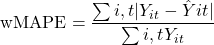
Finally, we measured the error between the actual sales volume () and the decimal prediction value () using MAE, RMSE, and the ratio error (wMAPE) that we get from the next formula:
Sensitivity and component ablations
The basic model originally used 14 observations and daily value 0.5. But in this test, we set the period to 7, 21, 28 observations and turned off the daily value as 0.0. In addition, we equally applied 0.5 rounding for every bread. If we turned on the stock out rule, we put modified sales numbers and set 0.25 equally for every weight. Finally, we changed the benchmark to 0.85, 0.90, and 0.95.
Results
Primary Store A performance
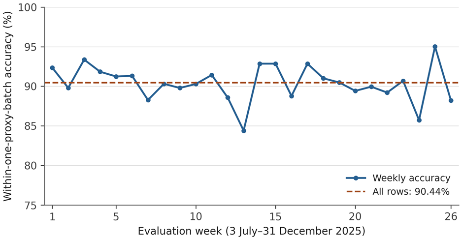
Every day, we predicted next-day sales for 182 straight days in Store A. We did not forcibly fill to 0 and just deleted 16 date-item pairs that did not have actual sold records among the original data. So we scored only based on a total of 4,810 rows that came from July 3 to December 31, 2025 (Figure 1). But we also excluded the first 28 rows (the first fold) from interval and review-gate evaluation, because they did not have prior past error data. Finally, we calculated the uncertainty band and review gate scores only based on the rest of the 4,782 rows (Table 1). We can see that 82.31% of actual sales came into the 80% prediction band that was made using only past fold errors, which was pretty similar to our target score of 80%.
| Measure | Result | Denominator or interpretation |
| Scored rows | 4,810 | 182 daily D+1 cutoffs |
| MAE | 1.87 units | Continuous center versus observed sales |
| RMSE | 8.84 units | Continuous center versus observed sales |
| wMAPE | 60.09% | Sum absolute error / sum observed sales |
| Exact proxy-batch accuracy | 57.90% | 4,810 rows |
| Within-one-proxy-batch accuracy | 90.44% | 4,810 rows |
| 80% residual-band coverage | 82.31% (3,936/4,782) | Prior-fold-calibrated rows |
| Guaranteed-shortfall row rate | 23.16% | Recommendation below observed sales |
| Guaranteed-shortfall units | 5,204 | Lower-bound shortfall versus completed sales |
| Potential-excess row rate | 30.98% | Recommendation above observed sales |
| Potential-excess units | 4,293 | Not observed waste |
| Retrospective review-trigger rate | 63.11% (3,018/4,782) | Calibration-eligible rows |
Error distribution and extreme-volume rows
Looking at Table 1, MAE is 1.87 but RMSE is 8.84, which means the difference is very big. This is not because we predicted badly every day. It is because there were some outliers where bread suddenly sold much more than on a normal day. Actually, the top 24 rows which is 0.5% that had the biggest squared error made up 89.2% of the sum of the total squared error. If we leave off only these 24 rows, RMSE decreases from 8.84 to 2.91, but MAE changes just from 1.87 to 1.49. And also, if we leave off the top 1% (48 rows), 92.0% of the total squared error disappears and RMSE drops down to 2.50. However, the POS data that we used did not have a catering or special event label. So we did not delete these big-number rows and we just kept them in our results.
Retrospective selective review
Among the 4,782 rows that we tested, 1764 at 36.89% went through automatically, and the rest 3018 at 63.11% were passed for human review. In Table 2, passed by itself rows have lower MAE and higher batch match rate agreement. In our systems’ actual pass rate 36.9%, automatic group accuracy within one batch was 95.6%. A random pick only gets 90.4%, so our result is much better. Still, a simple rule that only checks the range width gets 95.5% which is almost the same. If we raise the score limit, the share of rows that pass decreases but accuracy generally increases, with some reversals. For example, if we set the standard as 0.7, only 27.7% went through by themselves. But accuracy within one batch and the mistake rate became just 97.9%, 2.1%. But passing automatically and having a high trust score were not the same. 866 high score rows and 898 middle-score rows were mixed inside those 1764 rows. And among the 1153 high confidence, 287 rows were passed for human review because they were detected by other safety checks. In automatic groups, the rounded proxy-batch target was 0 in 73.6% of the rows, but review rows were 44.5%. If we only look at rows with a nonzero rounded proxy-batch target, there is little difference because accuracy was 84.1% and 84.5%.
| Route | Rows | Share | MAE (units) | Exact proxy-batch | Within one proxy batch |
| Auto-pass | 1,764 | 36.89% | 1.663 | 71.32% | 95.58% |
| Review-required | 3,018 | 63.11% | 1.993 | 50.03% | 87.44% |
Dense and sparse diagnostic
Looking at table 3, there is one interesting optical illusion. On the surface, occasionally sold breads’ accurate rate was 76.07% , so it looks much higher than popular breads’ 37.48%. However, this is because 96.54% of exact matches for occasionally sold bread had a zero rounded proxy-batch target and zero recommendation, compared with 0.24% for popular breads. So if we only calculate rows with a nonzero rounded proxy-batch target, the results were completely overturned. In this case, popular breads’ accurate match rate was 49.16% and within-one-batch accuracy was 87.52%.But occasionally sold bread dropped to 15.65% and 71.96%.( Popular bread and occasionally sold breads’ rate that came into the 80% prediction interval was 77.44%, 86.64%). 86.02% of Store A’s total sales came from these popular breads, and popular breads’(5.684) daily average sales were much higher than occasionally sold bread(0.822).So MAE is much bigger but wMAPE is much smaller. By the way, in store A ,all of the popular breads were in hero ranks so we can’t analyze the volume effect and the rounding effect separately.
| Segment | Rows | Sales share / zero proxy-batch target | MAE / wMAPE | Exact / within one |
| Dense | 2,265 | 86.02% / 23.93% | 3.060 / 53.83% | 37.48% / 85.08% |
| Sparse | 2,545 | 13.98% / 83.18% | 0.811 / 98.62% | 76.07% / 95.21% |
Store A model comparison
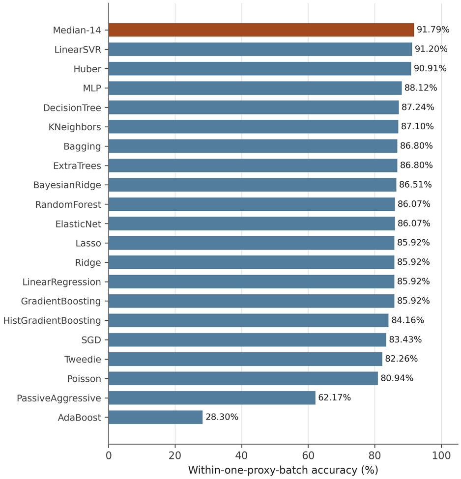
Table 4 was the result that pits our basic model(Median-14) against other 20 comparison models in store A. To summarize, in the within-one-batch accuracy rate, our model beat all of the predetermined 18 models even after statistical correction(adjusted p= 0.0020). Only LinearSVR and HuberRegressor models were not statistically meaningfully different from our model(Table 4; Figure 2). In this test, after deleting two combinations with empty data, every model equally predicted 682 rows about “Wednesday” 26 times and 34 breads. Here, our model’s batch accuracy rate was 58.80%(401/682), rate that falls within one batch was 91.79%(626/682), and error was MAE 1.70, RMSE 4.46, and wMAPE 56.62%.
| Model | Within one: Median-14 / model | Δ (pp; 95% CI) | Holm-adjusted p | Finding |
| Linear SVR | 91.79% / 91.20% | +0.59 [-0.28, +1.54] | 0.3894 | No clear difference |
| Huber | 91.79% / 90.91% | +0.88 [-0.29, +2.08] | 0.3894 | No clear difference |
Exploratory Store B rolling comparison
Table 5 was held in store B. Here, we need to consider that the sample size was small because we only used data from 8 Saturdays. Looking at the result, Huber model(78.70%) and LinearSVR models’(77.78%) 1- batch hit rate was much higher than our basic model(Median-14). DecisionTree(72.22%) model was not statistically much different from our model, and our model beat the rest 17 comparison models.
This comparison equally ran across 216 rows for 8 prediction days(all Saturday) and 30 breads with no missing records.Here, our Median-14 model’s batch matching accuracy was 50.00%(108/216), rate that matches within one batch was 73.15%(158/216), and error was MAE 2.05, RMSE 4.53, and wMAPE 51.31%.
| Model | Within one: Median-14 / model | Δ (pp; 95% CI) | Holm-adjusted p | Finding |
| Huber | 73.15% / 78.70% | -5.56 [-6.13, -5.00] | 0.0020 | Challenger higher |
| Linear SVR | 73.15% / 77.78% | -4.63 [-5.56, -3.70] | 0.0020 | Challenger higher |
| Decision tree | 73.15% / 72.22% | +0.93 [-1.89, +3.64] | 0.5262 | No clear difference |
Store B fixed-origin stress test
A large-scale stress test(Table 6) in store B came to the same conclusion as Store A’s main experiment. After the statistical correction( Block Bootstrap and Holm correction), there was no statistical difference with the top two models Huber(78.06%) and LinearSVR(77.00%) which were the most similar to our model. Our Median-14 model’s accuracy was higher than the other 18 machine learning models(adjusted p=0.0020). This test finished learning with data up to the end of 2025 and evaluated all 1,422 rows at once throughout 59 days in January and February 2026 and 26 breads(excluding 171 rows with no records). Here, our Median-14 model’s batch matching accuracy was 45.01%(640/1,422), rate that matches within one batch was 77.57%(1,103/1,422), and the error was MAE 1.95, RMSE 4.95, and wMAPE 64.34%.
| Model | Within one: Median-14 / model | Δ (pp; 95% CI) | Holm-adjusted p | Finding |
| Huber | 77.57% / 78.06% | -0.49 [-1.46, +0.43] | 0.4400 | No clear difference |
| Linear SVR | 77.57% / 77.00% | +0.56 [-0.34, +1.38] | 0.4400 | No clear difference |
Sensitivity and component ablation
Looking first at the results of the period (n) to find the median value in Table 7, no single period ranked first across all criteria at the same time. When we set it to 7 observations, every metric was the worst. 14 observations that we normally use had the highest batch accuracy(57.90%). Meanwhile, 21 observations’ 1-batch hit rate(90.91%) was the highest, and 28 observations’ MAE(1.847) and wMAPE(59.35%) were the lowest. These tests were comparing the Median-14 model in Store A’s same 4,810 rows to a single-variable model(Originally 16 names, removing the duplicates with the default values leaves a total of 10 distinct settings).
| n | Exact proxy batch; delta (pp) | Within one; delta (pp) | MAE; delta | wMAPE; delta (pp) |
| 7 | 57.01%; -0.89 | 89.65%; -0.79 | 1.925; +0.056 | 61.88%; +1.79 |
| 14 (primary) | 57.90%; 0 | 90.44%; 0 | 1.870; 0 | 60.09%; 0 |
| 21 | 57.55%; -0.35 | 90.91%; +0.48 | 1.854; -0.016 | 59.58%; -0.52 |
| 28 | 57.75%; -0.15 | 90.77%; +0.33 | 1.847; -0.023 | 59.35%; -0.74 |
Looking at the different settings in Table 8, if we used the 0.50 rounding method for every bread rather than rounding differently by ranks, batch accurate match rate and 1-batch hit rate increased by 1.68%p and 0.15%p even though the predicted number remained. However, if we turned off day of the week adjustment to 0.0, exact match rate and 1-batch hit rate decreased by 1.66%p and 1.00%p. We can know that every grade deteriorated noticeably.Especially, when we only looked at POS data and turned on Sell-out rule, all data performed worse than the model that learned on the original sales regardless of how we changed weight or Threshold(q)(dropping by 3.20%p to 6.32%p).
| Specification | Exact proxy batch; delta (pp) | Within one; delta (pp) | MAE; delta | wMAPE; delta (pp) |
| Primary: weekday shrinkage 0.5, raw POS target, service-profile rounding | 57.90%; 0 | 90.44%; 0 | 1.870; 0 | 60.09%; 0 |
| Weekday shrinkage 0.0 | 56.24%; -1.66 | 89.44%; -1.00 | 1.941; +0.071 | 62.38%; +2.29 |
| Heuristic-corrected target, default weights, q=0.90 | 53.95%; -3.95 | 90.04%; -0.40 | 1.916; +0.047 | 61.59%; +1.50 |
| Heuristic correction, equal 0.25 weights | 53.22%; -4.68 | 90.04%; -0.40 | 1.926; +0.056 | 61.89%; +1.80 |
| Heuristic correction, default weights, q=0.85 | 54.70%; -3.20 | 90.25%; -0.19 | 1.903; +0.033 | 61.16%; +1.07 |
| Heuristic correction, default weights, q=0.95 | 51.58%; -6.32 | 89.25%; -1.19 | 1.968; +0.098 | 63.23%; +3.14 |
| Common 0.50 rounding | 59.58%; +1.68 | 90.58%; +0.15 | 1.870; 0 | 60.09%; 0 |
POS-only stockout correction
To find out why out of stock correction that was based only on the POS record failed, we did an extra experiment(random seed 42) that made a fake out of stock situation. To get to the point, our Out-of-Stock Suspect Score was unable to distinguish between days when an actual stockout happened and normal days(ROC AUC 0.52, like a coin toss).Just looking at the day when stockout happened, correction rule decreased the error with original demand by 15.8%. But we couldn’t determine appropriately which day had a stockout, so we inflated sales needlessly across 55% of normal days. Because of this, if we calculate the sum of all rows, the adjusted number ( ) was actually much further away from the original demand (
 ) than the untouched number (
 ) ( Total MAE got worse from 0.23 to 0.73 after correction). When we did this experiment, we defined the original sales number as the true demand () and randomly selected 15% of the peak sales days (at or above the 60th percentile). Then we made fake stockouts by artificially suppressing sales with this method:

And based only on the reduced number (
), we checked how accurately the correction value () found the original number ().
Discussion
These results show that it serves as a robust baseline, performing on par with highly complex machine learning models. We can even see our Median-14 model’s calculating process in the POS data environment of a small bakery. (Of course, no statistical difference doesn’t mean that the two models are exactly the same, and keep in mind that this comparison was only based on Store A’s 26 Wednesdays of data and 1-batch hit rate). Reviewing the answers to the four questions we initially asked, in the test that changed settings one by one, no period between 7 and 28 observations ranked first in all aspects at the same time. Day of the week adjustment steadily increased grades, and general 0.5 rounding also slightly increased the batch match rate. But stockout correction that only used POS records rather decreased accuracy. The 80% prediction range made with past errors accurately captured 82.31% of the eligible rows. Review gate automatically passed through the rows with lower error by passing 63.11% of the eligible rows to human review. When we evaluated it in a direct row-by-row comparison with other machine learning models, there was no big difference between our model and the two linear models(LinearSVR, HuberRegressor). Also our model beat all 18 other models. This was also checked in both Store A’s weekly comparison and Store B ‘s stress test( But, both linear models performed better in the small-scale test for Store B, which looked at only 8 Saturdays). Finally, in store A’s main experiment ( 4,810 rows) conducted with complete prevention of data leakage, our Median-14 model provided recommendations within a 1-batch margin of actual sales in 90.44% of the total and MAE was 1.87 ( The high RMSE was primarily due to outliers in the top 0.5% of date-SKU rows ranked by squared error).
Interpreting the operational layers
From the design stage, our system was made for humans to understand the calculation process easily. Users can see step-by-step exactly how the recommended number was calculated, including the number of items sold over the last 14 observed open-day records, the day of week correction ratio, rounding criteria, the width of the prediction range, and the specific reason why it was passed to human review.
We set aside the breads that have insufficient or unstable data for human review, and looked at the records that were already incorrect in the past, and then set the risk range. Next, we decided the proxy batch count using the fixed proxy batch sizes and grade standards.On the other hand, our baseline model (Median-14) only calculated the number of breads sold the next day.
As seen in the previous test, all of those steps did not exist to increase the simple prediction accuracy.For example, although grade-specific rounding results in a slightly lower simple match rate compared to 0.50 rounding, it included the store’s operational strategy to avoid stockouts of its popular breads. Difference between popular bread and occasionally sold bread was combined not only because of how often it is sold, but also because of sales volume, the percentage of zero-sales days, batch sizes, and hero rank rounding for all popular breads. Also POS data alone fails to differentiate between early stockouts and low customer demand(AUC 0.52) , so turning on stockout correction without inventory records will unnecessarily inflate the forecast numbers even for normal days.
The review gate should also be viewed as a practical classification rule that chooses the bread the manager needs to check personally, and not as an AI that predicts the correct probability perfectly. As we increase the confidence score limit, the error generally decreases, but not at every threshold. But the reason why the accuracy of the automatically passed through group showed much higher results(95.58% vs 87.44%) in the comprehensive review gate was that the automatic pass group included many easy rows with a zero rounded proxy-batch target. Looking only at rows with a nonzero rounded proxy-batch target, accuracy of the two groups was almost same as 84.1%, 84.5%. So, as related studies16 indicate, when evaluating a review gate, we must look not only at overall accuracy but also consider the volume of work passed to humans, the risk of error, and the proportion of rows with a zero rounded proxy-batch target mixed in.
Recommendations
Before using the recommendations to plan actual production, bakeries should replace the estimated batch sizes and service tiers with recipe yields and documented store policies. Future data collection should include production quantities, inventory, sell-out times, and waste, so that we can evaluate whether the recommendations reduce shortages or leftovers. Weather forecasts should also be saved with their issue times to test what was actually available when each decision was made. A prospective study with managers should record decision time, changes to recommendations, product availability, waste, and cost. It should also check whether the explanations help managers recognize unreliable recommendations. Further comparisons should include stores from other brands, longer sales histories, and model tuning that uses only past data. These steps would test whether the results remain useful outside the current retrospective evaluation.
Limitations
This study used POS sales without records of production, inventory, sell-out times, waste, unmet requests, or manager actions. Therefore, we cannot estimate latent demand, actual waste, lost-sales costs, service levels, or profit. The shortage and leftover measures only describe differences from observed sales. Batch sizes and service tiers were estimated from past POS data, so proxy-batch accuracy does not measure agreement with actual production decisions. Both stores belong to the same brand, and the evaluation covers limited periods. Store B weather was synthetic, and neither dataset contained archived weather forecasts available at the decision time. The neutral weather inputs prevent future weather leakage but do not measure the value of real forecasts. The 20-model comparison used one fixed feature set without nested tuning, so different features, tuning, or longer histories could change the ranking. The review gate was tested only on historical data, and its effect on managers or store outcomes remains unknown. Repeated observations from the same products and dates also limit independence. Date-block resampling and multiple-comparison correction address part of this problem, but the Store B rolling comparison has only eight forecast dates. Its fixed-origin stress test mixes forecast horizons and does not reproduce repeated next-day deployment.
Conclusion
With POS-only operational data, a defensible batch-production system must be explicit about what is observed, what is proxied, and what is unavailable at decision time. The corrected evaluation shows how a transparent rolling-median core can be embedded in point-in-time data controls, proxy-batch discretization, walk-forward uncertainty estimation, and selective review. The contribution is not a claim that simple models always outperform complex models, nor that the system recovers latent demand or improves human decisions. It is a reproducible framework for producing and auditing next-day recommendations under severe data limitations, together with clear boundaries for the stronger operational claims that require inventory, waste, forecast-vintage, and user-study data.
References
- S. Nahmias. Demand estimation in lost sales inventory systems. Naval Research Logistics. Vol. 41, pg. 739-757, 1994, https://doi.org/10.1002/1520-6750(199410)41:6%3C739::AID-NAV3220410605%3E3.0.CO;2-A [↩]
- R. Anupindi, M. Dada, S. Gupta. Estimation of consumer demand with stock-out based substitution: An application to vending machine products. Marketing Science. Vol. 17, pg. 406-423, 1998, https://doi.org/10.1287/mksc.17.4.406 [↩]
- A. Jain, N. Rudi, T. Wang. Demand estimation and ordering under censoring: Stock-out timing is (almost) all you need. Operations Research. Vol. 63, pg. 134-150, 2015, https://doi.org/10.1287/opre.2014.1326 [↩]
- J. D. Croston. Forecasting and stock control for intermittent demands. Operational Research Quarterly. Vol. 23, pg. 289-303, 1972, https://doi.org/10.1057/jors.1972.50 [↩]
- A. A. Syntetos, J. E. Boylan. The accuracy of intermittent demand estimates. International Journal of Forecasting. Vol. 21, pg. 303-314, 2005, https://doi.org/10.1016/j.ijforecast.2004.10.001 [↩]
- R. H. Teunter, A. A. Syntetos, M. Z. Babai. Intermittent demand: Linking forecasting to inventory obsolescence. European Journal of Operational Research. Vol. 214, pg. 606-615, 2011, https://doi.org/10.1016/j.ejor.2011.05.018 [↩]
- L. J. Tashman. Out-of-sample tests of forecasting accuracy: An analysis and review. International Journal of Forecasting. Vol. 16, pg. 437-450, 2000, https://doi.org/10.1016/S0169-2070(00)00065-0 [↩]
- C. Bergmeir, R. J. Hyndman, B. Koo. A note on the validity of cross-validation for evaluating autoregressive time series prediction. Computational Statistics & Data Analysis. Vol. 120, pg. 70-83, 2018, https://doi.org/10.1016/j.csda.2017.11.003 [↩]
- H. Hewamalage, K. Ackermann, C. Bergmeir. Forecast evaluation for data scientists: Common pitfalls and best practices. Data Mining and Knowledge Discovery. Vol. 37, pg. 788-832, 2023, https://doi.org/10.1007/s10618-022-00894-5 [↩]
- S. Kapoor, A. Narayanan. Leakage and the reproducibility crisis in machine-learning-based science. Patterns. Vol. 4, pg. 100804, 2023, https://doi.org/10.1016/j.patter.2023.100804 [↩]
- S. Makridakis, E. Spiliotis, V. Assimakopoulos. The M4 Competition: Results, findings, conclusion and way forward. International Journal of Forecasting. Vol. 34, pg. 802-808, 2018, https://doi.org/10.1016/j.ijforecast.2018.06.001 [↩]
- V. Sillanpaa, J. Liesio. Forecasting replenishment orders in retail: Value of modelling low and intermittent consumer demand with distributions. International Journal of Production Research. Vol. 56, pg. 4168-4185, 2018, https://doi.org/10.1080/00207543.2018.1431413 [↩]
- R. Fildes, S. Ma, S. Kolassa. Retail forecasting: Research and practice. International Journal of Forecasting. Vol. 38, pg. 1283-1318, 2022, https://doi.org/10.1016/j.ijforecast.2019.06.004 [↩]
- R. A. C. M. Broekmeulen, K. H. van Donselaar. A heuristic to manage perishable inventory with batch ordering, positive lead-times, and time-varying demand. Computers & Operations Research. Vol. 36, pg. 3013-3018, 2009, https://doi.org/10.1016/j.cor.2009.01.017 [↩]
- F. M. M. Christensen, C. Solheim-Bojer, I. Dukovska-Popovska, K. Steger-Jensen. Developing new forecasting accuracy measure considering product’s shelf life: Effect on availability and waste. Journal of Cleaner Production. Vol. 288, pg. 125594, 2021, https://doi.org/10.1016/j.jclepro.2020.125594 [↩]
- R. El-Yaniv, Y. Wiener. On the foundations of noise-free selective classification. Journal of Machine Learning Research. Vol. 11, pg. 1605-1641, 2010, https://www.jmlr.org/papers/v11/el-yaniv10a.html [↩] [↩]
- H. Mozannar, D. Sontag. Consistent estimators for learning to defer to an expert. Proceedings of the 37th International Conference on Machine Learning. Vol. 119, pg. 7076-7087, 2020, https://proceedings.mlr.press/v119/mozannar20b.html [↩]
- G. Bansal, T. Wu, J. Zhou, R. Fok, B. Nushi, E. Kamar, M. T. Ribeiro, D. S. Weld. Does the whole exceed its parts? The effect of AI explanations on complementary team performance. Proceedings of the 2021 CHI Conference on Human Factors in Computing Systems. pg. 1-16, 2021, https://doi.org/10.1145/3411764.3445717 [↩]
- Z. Bucinca, M. B. Malaya, K. Z. Gajos. To trust or to think: Cognitive forcing functions can reduce overreliance on AI in AI-assisted decision-making. Proceedings of the ACM on Human-Computer Interaction. Vol. 5, pg. 1-21, 2021, https://doi.org/10.1145/3449287 [↩]
- C. Rudin. Stop explaining black box machine learning models for high stakes decisions and use interpretable models instead. Nature Machine Intelligence. Vol. 1, pg. 206-215, 2019, https://doi.org/10.1038/s42256-019-0048-x [↩]