A Cost Sensitivity Framework for Machine Learning Model Selection in Semiconductor Defect Detection

Abstract

Semiconductor manufacturing requires precise quality control, where even small defect rates significantly impact yield and profitability. In practice, the cost of missing a defective wafer may differ from the cost of triggering a false alarm. Motivated by this problem , this study develops a framework for selecting optimal machine learning models based on cost-sensitivity models in defect detection. Forty configurations using traditional and ensemble models, Logistic Regression (LR), Random Forest (RF), Support Vector Machine (SVM), Neural Network (NN), Easy Ensemble Classifier (EEC), and Balanced Random Forest Classifier (BRFC) were evaluated on  the UCI SECOM (Semiconductor Manufacturing) dataset containing 1,567 samples with 6.6% defect rate, and 590 features. Configurations spanned two preprocessing pipelines (with and without feature reduction) and two resampling strategies (none, SMOTE, and SMOTEENN). All preprocessing was performed strictly after train-test splitting, with transformations fitted only on training data to prevent information leakage. F1-score was used to shortlist the top 6 models as it balances precision and recall; subsequent analyses including statistical validation, feature importance, and cost-sensitivity were conducted on these models. EEC achieved the highest F1-score (0.22, 95% CI: 0.15 –0.29) and recall (62%), making it the best performer for minority class detection. However, cost-sensitivity analysis reveals that F1-score alone does not determine the optimal model. NN with SMOTE minimizes total cost in most operational scenarios including equal cost conditions and when false alarms are expensive due to its higher precision (25% vs 13%). EEC becomes optimal when missed defects cost 10× or more than false alarms, where its superior recall outweighs the higher false alarm rate. Statistical analysis showed overlapping confidence intervals among top models, indicating no significant performance differences reinforcing that model selection should be driven by operational cost structure rather than F1-score ranking alone.

Keywords: SECOM dataset, Easy Ensemble Classifier, Balanced Random Forest, class imbalance, precision, recall, F1-score, cost-sensitive learning

Introduction

Semiconductor manufacturing is a very precision-dependent industry that involves hundreds of intricate step sensor readings that must be executed flawlessly. Even minor deviations in process parameters, or equipment performance can lead to wafer defects, reducing yield and driving up production costs. As AI rapidly advances  powering technologies from conversational agents to self-driving cars, medical diagnostics and robotics the demand for faster, more efficient, and reliable semiconductor chips continues to grow. With growing global demand for chips in order to  avoid supply shortage , improving manufacturing efficiency is critical.

 A core challenge in semiconductor defect detection is extreme class imbalance: the vast majority of wafers pass inspection, while defective wafers are rare. This creates a problem where machine learning models can achieve high accuracy by simply predicting “pass” for everything—while failing to detect the defects that actually matter.

The SECOM dataset (Semiconductor Manufacturing) is a publicly available dataset from a real semiconductor fabrication facility, introduced by McCann and Johnston¹, has become a benchmark for studying this challenge. It contains 1,567 production records with 590 sensor variables, classified as either pass (1,463 samples, 93.4%) or fail (104 samples, 6.6%). One important aspect of this dataset is that the 590 sensor variables are represented only by numerical indices rather than descriptive names. This anonymization was done to protect the proprietary details of the semiconductor manufacturing process, as the original sensor identities (e.g., machine parameters, chemical measurements) are considered confidential.

This study makes two distinct contributions: (1) Rigorous methodology with all preprocessing performed after train-test splitting and transformations fitted only on training data which some prior studies had missed along with complete minority class metrics (precision, recall, and F1) with 95% confidence intervals from cross-validation. Without minority class reporting, high accuracy may just mean predicting the majority and without confidence intervals, apparent performance differences between models may simply reflect random variation. (2) A practical cost-sensitivity framework that helps practitioners select models based on their operational cost structure, specifically whether the cost of missed defects outweighs the cost of false alarms or vice versa.

Literature Review

Foundational Studies (2008-2017)

McCann and Johnston¹ introduced the SECOM dataset in 2008 which has been studied and analysed over the years in many research papers. Kerdprasop and Kerdprasop² and Munirathinam and Ramadoss³ have conducted extensive work on the SECOM dataset, applying feature selection methods such as Principal component analysis (PCA), chi-square tests, correlation analysis and Variance Inflation Factor (VIF) , along with a range of models including Decision Tree (DT), Naïve Bayes (NB), k-Nearest Neighbor (KNN), LR, Artificial Neural Networks (ANN) and SVM (precision=0.47, recall=1.00, F1=0.61)—perfect recall suggests contamination.

Recent SECOM Studies (2018-2024)

Salem et al.⁴ conducted the most methodologically rigorous preprocessing evaluation, testing 288 combinations of data pruning, imputation, feature selection, and classification methods. They performed train-test splitting before imputation to prevent data leakage. Their ‘In-painting KNN-Imputation’ technique achieved 65.38% recall and 70.22% AUC with LR. Lee et al. ⁵ proposed a data-driven approach for identifying critical process steps using Expectation-Maximization (EM) algorithm imputation, SMOTE resampling and MeanDiff-based feature selection, focusing on feature relevance rather than classification performance optimization. While demonstrating novel ensemble optimization, minority class-specific metrics were not isolated. Moldovan et al. ⁶ introduced a PSO-optimized ensemble of deep neural networks (DNNs) for SECOM classification which determined optimal weights for combining multiple DNN models. Cho et al.⁷ compared seven imputation methods with six resampling techniques including Generative Adversarial Network (GAN) based oversampling.Yousef et al.⁸ have focused on feature  reduction using CfsSubsetEval and dimensionality reduction via PCA, reducing features to 168 and applying NB, DT, Multilayer Perceptron (MLP), and SVM models, evaluated against five metrics (TP rate, FP, precision, F-measure, and accuracy).Swathi et al.⁹ applied SMOTE for class balancing before train-test split, which causes data leakage and inflates their reported metrics (99.4% SVM accuracy, 99.1% RF accuracy). Pradeep et al.¹⁰ frame semiconductor fault prediction as a supervised classification problem using Random Forest–centric pipelines, achieving very high reported accuracy by optimizing tree depth and feature subsets. Zhai et al.¹¹ proposed xAutoML, treating missing value patterns as signals rather than noise, expanding the original 590 features to over 60,000 domain-informed features. Farrag et al.¹² proposed a rare-class prediction framework using consensus-based feature selection with multiple heterogeneous methods (Boruta, MARS, mutual information, ANOVA, RFE, LASSO, sequential selection) using voting-based feature retention. Moldovan et al. ¹³ applied Boruta and MARS algorithms for feature selection combined with undersampling and Random Forest classification. Park et al.¹⁴ used LR, SVM, and Extreme Gradient Boosting (XGB), combined with preprocessing and feature selection techniques such as Pearson correlation coefficient–based selection (reducing to 12 features) and various resampling methods, including advanced sampling based selection methods to handle class imbalance .Using accuracy, recall, and specificity as metrics and geometric mean of recall & specificity, the authors evaluated 150 combinations and identified SVM with ADASYN oversampling and MaxAbs scaling as the best-performing configurations.

Cost-Benefit Studies

Van Kollenburg et al.¹⁵ approached the problem from a cost-benefit perspective through ‘predictive discarding’ aborting production when failure is predicted. They demonstrated that even weak predictors (recall <50%) provide economic benefit when downstream costs are high, establishing the theoretical foundation for cost-sensitivity analysis. Presciuttini et al.¹⁶ introduced an interpretable ML framework using LIME for sample-specific explanations, enabling operators to understand why a wafer fails. Due to computational costs, explanations were generated for only a subset of samples.

Identified Gaps

Three critical gaps emerge from this literature review. First, several studies apply preprocessing before train-test splitting, potentially getting results through data leakage. This has been called out and addressed by Park et al.¹⁷  too. Second, no prior study reports complete minority class metrics (precision, recall and F1) with statistical confidence intervals. Third, no existing study covers the practical, cost-based application of any model. This paper bridges that gap through a cost-sensitivity analysis demonstrating real-life applicability, supported by rigorous methodology and comprehensive reporting. Table 1 depicts a consolidated literature review of 15 papers on SECOM dataset

Study	Year	Leakage Prev.	Imbalance Strategy	Accuracy	Precision	Recall/TPR	F1	AUC	Best Model
Kerdprasop et al.2	2011	Unclear	Boosting	—	0.47 (M)	1.00 (M)*	0.61 (M)*	—	DT + Boosting
Munirathinam et al.3	2016	Unclear	SMOTE	—	0.90 (O)	0.90 (O)	0.95 (O)	—	KNN
Salem et al. 4	2018	Yes ✓	SMOTE	—	0.157 (M)	0.654 (M)	—	0.702	LR
Lee et al.5	2019	Unclear	None	—	—	—	—	—	Feature Selection
Moldovan et al.6	2020	Unclear	None	—	—	—	—	—	PSO-DNN
Cho et al.7	2022	No ✗	GAN, SMOTE	—	—	—	0.915 (W)	—	Various ML
Yousef et al.8	2020	Unclear	None	0.91	0.91 (O)	0.91 (O)	—	—	MLP
Swathi et al.9	2024	Unclear	None	—	—	—	—	—	ML Ensemble
Pradeep et al.10	2023	Unclear	None	0.94	—	1.00 (O)*	0.97 (O)	—	RF
Zhai et al.11	2024	Unclear	None	—	—	—	—	—	xAutoML
Farrag et al.12	2024	Unclear	k-NN impute	—	0.66 (M)	0.96 (M)*	—	—	ML Ensemble
Moldovan et al.13	2017	Unclear	Undersampling	—	0.915 (?)	—	—	—	RF + Boruta
Park et al. 14	2024	Yes ✓	ADASYN	0.85	—	0.64 (M)	—	0.73 GM	SVM + ADASYN
van Kollenburg et al.15	2022	N/A	None	—	—	—	—	—	Various (Cost)
Presciuttini et al.16	2024	Unclear	None	—	—	—	—	—	XGBoost (LIME)
This Paper	2025	Yes ✓	Balanced Ensembles	0.71	0.134 (M)	0.62 (M)	0.220 (M)	—	EEC, BRFC

(M) = Minority class metrics — Performance on the 6.6% defective wafers specifically (true defect detection capability)

(O) = Overall/macro metrics — Averaged across both classes; high values can mask poor minority detection due to 93.4% majority class. (W) = Weighted F1 — Weighted by class support, not minority-specific . (?) = Unclear — Original paper does not specify whether minority or overall metrics. GM = Geometric Mean of Sensitivity and Specificity; — = Not reported; * = Potentially biased metric.

Key Observations:

1. Studies reporting (O) overall metrics show inflated performance (0.90+) because the 93.4% majority class dominates. 2. Only two studies^{18 ,19} explicitly preventsdata leakage. 3. Moldovan et al.²⁰ reported 0.915 precision using undersampling with Boruta and RF, but metric type (minority vs overall) is unclear.

4. Many studies do not clearly specify whether reported metrics are for minority class or overall, making direct comparison difficult.

Methodology

Experimental Design

Figure 1 presents the complete experimental methodology. The critical design principle is that all preprocessing occurs after the initial train-test split, and all transformations (imputation, scaling) are fitted only on training data then applied to test data. This prevents any information from test samples leaking into the training process for all models. Following steps were followed (1) Columns with > 55% missing data were removed (2)  train-test split (80/20) was split.(3) Median imputation fitted on training data only (4) Robust scaling fitted on training data only , less sensitive to outliers, with parameters fitted only on the training data. After this two preprocessing pipelines were developed. Pipeline A (566 features): This pipeline focuses on data cleaning and scaling without aggressive feature reduction beyond initial missing value handling. Pipeline A had 566 features, two resampling methods were applied which are explained in sec 3.4. Pipeline B (208 features):This pipeline builds upon Pipeline A by performing additional aggressive feature reduction steps.(5) Remove features with zero variance (6) Remove features with >0.95 Pearson correlation.(7) Features exhibiting high Variance Inflation Factor (VIF) scores (indicating multicollinearity above a threshold of (5) are iteratively removed until all remaining features have VIF below the threshold. Pipeline B had 208 features, two resampling methods were applied which are explained in sec 3.4.

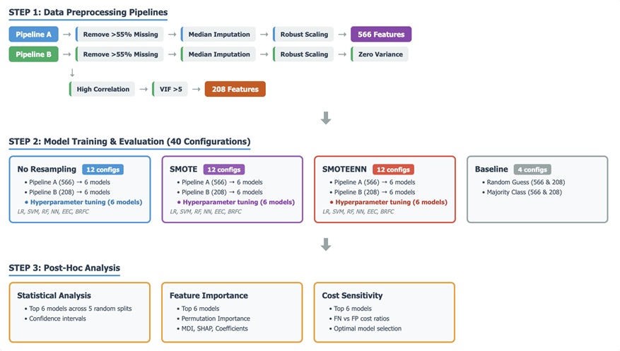
Models and Hyperparameters

 All six models were evaluated using RandomizedSearchCV with 2-fold stratified cross-validation on the training data. This approach explores the hyperparameter space by sampling a fixed number of combinations (n_iter=10). Parallel computation (n_jobs=-1) was enabled to accelerate the search process. Each model’s hyperparameter tuning strategy is detailed below, whereas foundation principles of BRFC and EEC are explained as these models are less common. Table 2 shows the  Hyperparameter Tuning parameters for the 6 models.

Logistic Regression (LR) – Hyperparameter Tuning applied : The tuning process focused on C, the inverse regularization strength that controls overfitting, along with the penalty type (l1 or l2) and the solver (liblinear or saga), which determines the optimization algorithm and its compatibility with different penalties.

Random Forest Classifier (RF) – Hyperparameter Tuning applied- `n_estimators` (the number of trees in the forest), `max_depth` (the maximum depth of each tree, controlling complexity), `min_samples_split` (the minimum number of samples required to split an internal node), and `max_features` (the number of features to consider when looking for the best split).

Support Vector Machine (SVM) – Hyperparameter Tuning: Tuning involved C (the regularization parameter balancing misclassification against decision boundary smoothness), gamma (kernel coefficient defining the influence of individual training examples), and kernel type (rbf and polynomial) to find the optimal decision boundary.

Neural Network (NN) – Hyperparameter Tuning – Optimization focused on the network architecture  (hidden_layer_sizes), activation function (relu or tanh for non-linearity), alpha (L2 regularization to prevent overfitting), and learning rate strategy (constant or adaptive) to control step size during weight updates.

Easy Ensemble Classifier (EEC) – An ensemble technique for class imbalance by repeatedly training multiple base estimators on different balanced subsets of the training data. Each subset is created by randomly selecting a portion of the majority class and combining it with all samples from the minority class. The final prediction is made by combining the predictions of these base estimators. Figure 2 shows the working of EEC.  Hyperparameter Tuning- `n_estimators` (the number of base estimators in the ensemble) and `sampling_strategy` (determining how the majority class samples are selected for each subset, e.g., `auto`, `majority`, `not minority`).

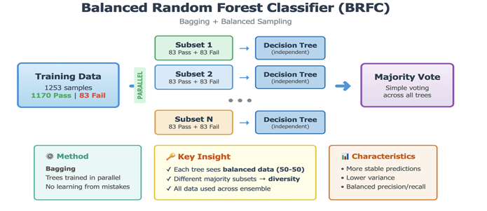
Balanced Random Forest Classifier (BRFC)-A variant of the Random Forest algorithm for imbalanced datasets. Each bootstrap sample for building individual trees is drawn in a way that balances the class distribution. It oversamples the minority class and undersamples the majority class to create balanced subsets for tree training, enhancing the model’s sensitivity to the minority class. Figure 3 shows the working of BRFC. Hyperparameter Tuning:Optimized parameters included `n_estimators` (the number of decision trees), `max_depth` (the maximum depth of each tree, controlling complexity), `min_samples_split` (the minimum number of samples required to split an internal node), and `max_features` (the number of features considered for the best split).

Resampling

Three conditions were tested on Pipeline A (566 features) and Pipeline B(208 features): (1) None – no synthetic resampling; (2) SMOTE – Synthetic Minority Over-sampling Technique; (3) SMOTE-ENN – SMOTE followed by Edited Nearest Neighbors. SMOTE is a resampling method that generates synthetic samples for the minority class by interpolating between existing minority class instances. It is used to address class imbalance. SMOTE-ENN: SMOTE + Edited Nearest Neighbors. ENN removes samples misclassified by neighbors, cleaning noisy boundaries. A baseline model  was also evaluated.  These baselines help confirm that our more advanced models are genuinely contributing to better predictive performance, especially for the challenging minority class.

Evaluation

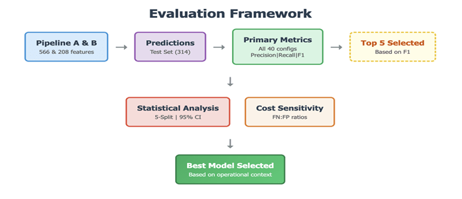
The evaluation framework depicted in Figure 4 addresses both methodological rigor and practical utility . Minority class metrics (precision, recall, F1) assess defect detection capability. Top 6 models were selected on the basis of F1-score, the same models were assessed for statistical reliability using 95% confidence intervals from 5-split cross-validation. Cost-sensitivity analysis for the same top 6 models was checked.Cost-sensitivity analysis enables practitioners to select models based on their operational cost structure.

Model	Hyperparameters
LR	C:[0.001-100], penalty:[l1,l2], solver:[liblinear,saga]
RF	n_estimators:[100-300], max_depth:[10,20,30,None], min_samples_split:[2,5,10]
SVM	C:[0.1-100], kernel:[rbf,poly], gamma:[scale,auto,0.01,0.1]
NN	hidden_layers:[(50,),(100,),(100,50)], activation:[relu,tanh], alpha:[0.0001-0.01]
EEC	n_estimators:[10,20,30], sampling_strategy:[auto,majority,not minority]
BRFC	n_estimators:[100-300], max_depth:[10,20,None], min_samples_split:[2,5]

Precision: When the model predicts a failure, how often is it correct? High precision means fewer false alarms. TP/(TP+FP).

Recall: Of all actual failures, how many did the model detect? High recall means fewer missed defects. TP/(TP+FN).

F1-Score: Harmonic mean of precision and recall: 2×(P×R)/(P+R).95% CI: Range where true F1 falls 95% of time. From 5-fold CV: Mean±1.96×SE. Overlapping CIs = no significant difference.

Nomenclature: Model_Features_Resampling. E.g., ‘EEC_566_None’ = Easy Ensemble, 566 features, no resampling.

Results

Overall Performance

Table 3 presents results for top-performing configurations. Complete results for all 40 configurations are provided in Appendix B, Table A. The best hyperparameters that led to the selection of top 6 models are tabulated in Appendix B, Table B. The top performing model based on F1 score is EEC with all 566 features and no resampling ,NN_566_SMOTE is not selected despite similar F1 because of low recall and  Its 95% CI includes negative values [-0.04, 0.30], indicating instability. EEC has tighter, all-positive CI [0.15, 0.29].

Config	Acc	Prec	Recall	F1	95% CI
EEC_566_None	0.71	0.13	0.62	0.22	[0.15,0.29]
NN_566_SMOTE	0.91	0.25	0.19	0.22	[-0.04,0.30]
BRFC_208_None	0.88	0.19	0.24	0.21	[0.08,0.32]
EEC_208_None	0.69	0.13	0.62	0.21	[0.17,0.28]
LR_208_SMOTEENN	0.76	0.13	0.48	0.21	[0.06, 0.23]
NN_208_SMOTEENN	0.76	0.13	0.48	0.21	[-0.07, 0.21]

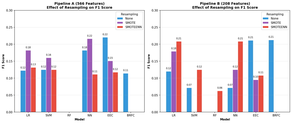
Impact of Feature reduction: Out of 36 configurations (18-Pipeline A, 18-pipeline B), only 4 benefitted from feature reduction from 566 to 208 but 3 out of those 4 are in top 6 performing models. In the case of RF the F1-score was 0 and the improved score is also too low. Models that benefited are highlighted in Table 4.

Model	Resampling	F1 (566)	F1 (208)	Improvement
BRFC	None	0.114	0.213	+0.099
NN	SMOTEENN	0.111	0.208	+0.097
LR	SMOTEENN	0.132	0.208	+0.077
RF	SMOTEENN	0.000	0.063	+0.063

Impact of Resampling Strategies

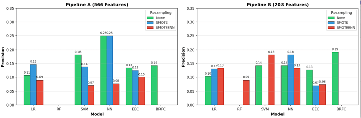
In Pipeline A (566 features), the high-dimensional feature space is sparse, allowing SMOTE-generated synthetic samples to spread without overlapping the majority class. In Pipeline B (208 features), the reduced feature space is denser and more compact, increasing the risk of synthetic samples overlapping with the majority class. SMOTEENN addresses this by applying an ENN cleaning step to remove noisy borderline samples. Traditional models (LR, SVM, NN) benefited from resampling, particularly on high-dimensional data. SMOTE improved F1-score for LR_566 (0.12→0.18), SVM_566 (0.13→0.16), and NN_566 (0.18→0.22). This improvement was driven primarily by recall gains—SVM_566 with SMOTEENN achieved 0.48 recall (vs 0.10 baseline)—though often at the cost of precision (0.18→0.07 for SVM_566_SMOTEENN). On reduced features (Pipeline B), SMOTEENN was more effective, with LR and NN both achieving F1=0.21.Ensemble models (EEC, BRFC) were hurt by resampling. These models already handle class imbalance internally through balanced bootstrapping, and adding synthetic samples disrupted their performance. EEC F1-score dropped from 0.22 to 0.15 with SMOTE, with recall falling from 0.62 to 0.19. BRFC failed completely (F1=0) with any resampling on both pipelines. Figures 5, 6, and 7 show the impact of resampling on F1-score, Precision, and Recall respectively. Full details are provided in Appendix Table B.

Statistical Analysis

Overlapping intervals: Five-split cross-validation for the top 6 models is shown in Table 5  reveals that no model achieves statistically superior minority F1 performance.

Model	F1	F2	F3	F4	F5	Mean±SD
EEC_208_None	0.19	0.27	0.23	0.24	0.20	0.23±0.03
NN_566_SMOTE	0.22	0.24	0.10	0.00	0.11	0.13±0.10
BRFC_208_None	0.30	0.17	0.21	0.22	0.23	0.22±0.05
EEC_566_None	0.22	0.27	0.21	0.23	0.16	0.22±0.04
LR_208_SMOTEENN	0.15	0.15	0.16	0.20	0.07	0.15±0.05

Cost-Sensitivity

This framework enables practitioners to select models based on their specific operational context.  Table 6 and 7 depicts bidirectional cost sensitivity of Top 6 models (based on F1- score ).

Total Cost = (FN × Cost_FN) + (FP × Cost_FP).

 Case 1: FN/FP ratio = 1, 5, 10, 25, 50, 100 (FN is more expensive). Cost = (FN × ratio) + (FP × 1). Ratios: 10:1 means FN costs 5× more than FP

• Missing defects is costly → High Recall is important
• Semiconductor context: A missed defect reaches customer = bad
• Optimal model at ratio s≥ 10:1 : EEC_566_None

Config	FN	FP	1:1	5:1	10:1	25:1	50:1	100:1
EEC_566_None	8	84	92	124	164	284	484	884
NN_566_SMOTE	17	12	29	97	182	437	862	1712
BRFC_208_None	16	21	37	101	181	421	821	1621
EEC_208_None	8	89	97	129	169	289	489	889
LR_208_SMOTEENN	11	65	76	120	175	340	615	1165
NN_208_SMOTEENN	11	65	76	120	175	340	615	1165

Case 2: FP/FN ratio = 1, 5, 10, 25, 50, 100 (FP is more expensive).Cost = (FN × 1) + (FP × ratio).Ratios: 1:5 means FP costs 5× more than FN

• False alarms are costly → High Precision is important
• Semiconductor context: Unnecessary inspection/rework = expensive
• NN is a better model at FP:FN ratio >=1

Config	FN	FP	1:1	1:5	1:10	1:25	1:50	1:100
EEC_566_None	8	84	92	428	848	2108	4208	8408
NN_566_SMOTE	17	12	29	77	137	317	617	1217
BRFC_208_None	16	21	37	121	226	541	1066	2116
EEC_208_None	8	89	97	453	898	2233	4458	8908
LR_208_SMOTEENN	11	65	76	336	661	1636	3261	6511
NN_208_SMOTEENN	11	65	76	336	661	1636	3261	6511

Feature Importance

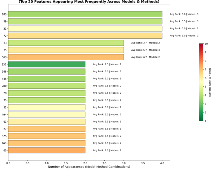
Feature importance analysis identifies which input variables (features) have the most influence on the model’s predictions ranking features from most to least important, This helps explain why a model predicts defects and which measurements matter most for quality control. Feature importance was computed using multiple methods for top 6 models only. 1.Permutation Importance(PI) – Model-agnostic 2. Mean Decrease Impurity(MDI) – Works on tree-based models i.e BRFC 3. Shapley Additive explanations (SHAP) Values – Works on LR, NN (not EEC, compatibility issues in BRFC ) 4. Coefficient Magnitude(CM) – Works on LR only. Overall 10 combinations were built. The results were consolidated and then a ‘consensus’ was built. This involves 1) Counting how many times each feature appears in the top 10 most important features across all model-method combinations. 2) Calculating the average rank for each feature. Step 1 has a priority over 2 . Figure 6 shows the top 20 consensus features by frequency of appearance across model-method combinations. The X-axis represents the number of appearances, and the Y-axis indicates the feature number. Average rank and unique model count are annotated for each feature.

Baseline Results

The results of baseline models are shown in Table 8. Any useful model must beat these. Of the 36 tuned model configurations, 26 outperformed the stratified random baseline, while 10 failed to detect any defects performing no better than the majority classifier.

Model	Accuracy	Precision	Recall	F1
Majority (all pass)	0.93	0.00	0.00	0.00
Stratified Random	0.87	0.05	0.05	0.05
Best (EEC)	0.71	0.13	0.62	0.22

Discussion

Model Selection Guidelines

Based on the results, final model guidance can be based on cost sensitivity. Other factors like feature reduction , resampling strategy and statistical analysis can be used to select the top few models for deeper analysis.

Cost sensitivity: When missed defects are costly (FN/FP ≥ 10:1), EEC_566_None minimizes total cost with its high recall (62%). When false alarms are costly (any FP/FN ratio), NN_566_SMOTE is optimal due to its higher precision (25%) and fewer false positives. Overall NN is a better model unless cost missed defects is 10 times more expensive than cost of unnecessary inspection, indicating that a model with high precision(NN) is more important than a model with higher recall (EEC), hence higher F1-score can be a factor to shortlist top models but cost sensitivity is recommended used to finalise the best model.

Feature Reduction: Only 4 of 36 configurations benefited from feature reduction, but 3 of these (BRFC_208_None, LR_208_SMOTEENN, NN_208_SMOTEENN) ranked in the top 6 by F1-score—indicating that when feature reduction helps, the improvement is substantial. Removing highly correlated features (>0.95 correlation) and multicollinear features (VIF>5) provided a cleaner feature space with less redundant sensor noise. This also improves feature importance interpretation: in Pipeline A, importance gets distributed across correlated sensors (e.g., Features 48-51 if nearly identical), whereas Pipeline B concentrates importance on representative sensors. For practical deployment, features important across both pipelines are most reliable; for Pipeline A models, manufacturers should monitor any representative sensor from each important correlated cluster.

Resampling Strategy : Traditional models (LR, SVM, NN) benefit from resampling as they lack inherent imbalance-handling mechanisms.Infact 3 out of top 6 models are traditional models on which resampling was applied.  SMOTE was more effective on full features (566), while SMOTEENN worked better on reduced features (208). However, resampling generally improves recall at the cost of precision. This occurs because synthetic minority samples make models more aggressive in predicting defects, catching more true positives but also generating more false alarms.In contrast, ensemble models (EEC, BRFC) that already handle imbalance internally through balanced bootstrapping were hurt by resampling—both precision and recall decreased due to noise introduced by synthetic samples. The cost-sensitivity framework in Section 4.5 provides guidance for selecting models based on these trade-offs.

Statistically superior: All top-performing models have overlapping 95% confidence intervals. This critical finding means that small F1 differences in published comparisons may not reflect true model superiority. Model selection should therefore be driven by operational requirements (cost structure, interpretability) rather than point-estimate rankings alone.

Why is the precision of our models so low?

A critical question emerges: why do our best models EEC and NN based on F1- score and cost-sensitivity analysis achieve only 13.% and 25% precision respectively. Several factors explain this:

(1) Fundamental data limitation: With only 104 defective wafers out of 1,567 (6.6%), the minority class provides limited examples for learning discriminative patterns.

(2) Recall-precision trade-off: EEC achieves 62% recall by being aggressive in flagging potential defects, which reduces false negatives (missed defects) but necessarily increases false positives (false alarms), resulting in lower precision (13%). Models with higher precision ( NN.at 25%) achieve this by being more conservative, but consequently miss more defects (19% recall).

(3) Comparison with prior work:  Park et al.²¹ achieved 64% recall under leakage-free conditions, nearly identical to our 62%. Salem et al.⁴ achieved 65% recall and 15.7% precision with their best configuration. This convergence suggests ~60-65% recall may represent the realistic ceiling for this dataset.

Limitations

This study has several limitations that should guide interpretation and future work:

(1) Small minority class: Only 21 defective wafers in the test set creates high variance in metrics. The wide confidence intervals reflect this uncertainty.

(2) Single dataset: Results are specific to this semiconductor facility. Different facilities with different processes, sensors, and defect types may show different model rankings.

(3) Anonymous features: The 590 features are anonymized (Feature 1 through Feature 590), preventing domain-specific feature engineering or interpretation of which sensors matter most.

(4) No temporal validation: We used random train-test splits rather than temporal splits (train on earlier data, test on later). In practice, manufacturing processes drift over time, and temporal validation would better estimate real-world performance.

(5) Limited deep learning exploration: While we included Neural Networks, we did not explore more sophisticated architectures (CNNs, LSTMs, Transformers) that might capture complex sensor interactions.

Conclusion

This study introduces a cost-sensitivity framework for selecting defect detection models based on operational cost structures rather than F1-score alone. Future work can validate these findings on larger, non-anonymized semiconductor datasets with temporal validation. All code and results are available to support reproducibility and future research as shared in the Appendix A and B.

Acknowledgments

“A preliminary version of this work focusing on model performance comparison was accepted at ICMLSC 2026 (https://icmlsc.org/) titled “Enhancing Failure Detection in Semiconductor Manufacturing using Balanced Random Forest Model”. This paper substantially extends the analysis by introducing a cost-sensitive decision framework.

Appendix

APPENDIX A: https://github.com/gandhidaksh/SECOMDATASETMLMODELS

APPENDIX B: Complete Results (All 40 Configurations)

Config	Acc	Prec	Recall	F1
EEC_566_None	0.71	0.13	0.62	0.22
NN_566_SMOTE	0.91	0.25	0.19	0.22
BRFC_208_None	0.88	0.19	0.24	0.21
EEC_208_None	0.69	0.13	0.62	0.21
LR_208_SMOTEENN	0.76	0.13	0.48	0.21
NN_208_SMOTEENN	0.76	0.13	0.48	0.21
LR_566_SMOTE	0.86	0.15	0.24	0.18
NN_566_None	0.91	0.25	0.14	0.18
LR_208_SMOTE	0.82	0.13	0.29	0.18
SVM_566_SMOTE	0.87	0.14	0.19	0.16
EEC_566_SMOTE	0.86	0.13	0.19	0.15
LR_566_SMOTEENN	0.79	0.09	0.24	0.13
SVM_208_SMOTEENN	0.91	0.18	0.10	0.13
SVM_566_None	0.91	0.18	0.10	0.13
SVM_566_SMOTEENN	0.55	0.07	0.48	0.13
NN_208_SMOTE	0.91	0.18	0.10	0.13
LR_566_None	0.86	0.11	0.14	0.12
LR_208_None	0.86	0.10	0.14	0.12
EEC_566_SMOTEENN	0.86	0.10	0.14	0.12
BRFC_566_None	0.90	0.14	0.10	0.11
NN_566_SMOTEENN	0.80	0.08	0.19	0.11
EEC_208_SMOTEENN	0.79	0.08	0.19	0.11
EEC_208_SMOTE	0.82	0.07	0.14	0.10
NN_208_None	0.92	0.14	0.05	0.07
SVM_208_None	0.92	0.14	0.05	0.07
RF_208_SMOTEENN	0.90	0.09	0.05	0.06
Baseline_Random_208	0.87	0.05	0.05	0.05
Baseline_Random_566	0.87	0.05	0.05	0.05
RF_208_None	0.93	0.00	0.00	0.00
RF_566_None	0.93	0.00	0.00	0.00
RF_566_SMOTEENN	0.92	0.00	0.00	0.00
RF_566_SMOTE	0.93	0.00	0.00	0.00
SVM_208_SMOTE	0.93	0.00	0.00	0.00
RF_208_SMOTE	0.93	0.00	0.00	0.00
BRFC_566_SMOTEENN	0.93	0.00	0.00	0.00
BRFC_566_SMOTE	0.93	0.00	0.00	0.00
BRFC_208_SMOTEENN	0.91	0.00	0.00	0.00
BRFC_208_SMOTE	0.93	0.00	0.00	0.00
Baseline_Majority_566	0.93	0.00	0.00	0.00
Baseline_Majority_208	0.93	0.00	0.00	0.00

Rank	Model	F1-score	Best Parameters
1	EEC_566_None	0.2203	sampling_strategy=auto; n_estimators=30
2	NN_566_SMOTE	0.2162	learning_rate=constant; hidden_layer_sizes=(100,50); alpha=0.0001; activation=relu
3	BRFC_208_None	0.2128	n_estimators=200; min_samples_split=5; max_features=sqrt; max_depth=20
4	EEC_208_None	0.2114	sampling_strategy=auto; n_estimators=20
5	LR_208_SMOTEENN	0.2083	solver=liblinear; penalty=l1; C=10
6	NN_208_SMOTEENN	0.2083	learning_rate=constant; hidden_layer_sizes=(100,50); alpha=0.001; activation=relu

References

1. M. McCann and A. Johnston, SECOM Dataset, UCI Machine Learning Repository, 2008, https://doi.org/10.24432/C54305. [↩] [↩]
2. K. Kerdprasop and N. Kerdprasop, Feature Selection and Boosting Techniques to Improve Fault Detection Accuracy in the Semiconductor Manufacturing Process, Proceedings of the International MultiConference of Engineers and Computer Scientists (IMECS), Hong Kong, 2011, https://www.iaeng.org/publication/IMECS2011/. [↩]
3. S. Munirathinam and B. Ramadoss, Predictive Models for Equipment Fault Detection in the Semiconductor Manufacturing Process, International Journal of Engineering and Technology, Vol. 8, pg. 273–285, 2016, https://doi.org/10.7763/IJET.2016.V8.898. [↩]
4. M. Salem, S. Taheri, and J.-S. Yuan, An Experimental Evaluation of Fault Diagnosis from Imbalanced and Incomplete Data for Smart Semiconductor Manufacturing, Big Data and Cognitive Computing, Vol. 2, no. 4, Article 30, 2018, https://doi.org/10.3390/bdcc2040030. [↩] [↩]
5. D. H. Lee, J. K. Yang, C. H. Lee, K. J. Kim, A Data-driven Approach to Selection of Critical Process Steps in the Semiconductor Manufacturing Process Journal of Manufacturing Systems, Vol. 52, 146-156, 2019, https://doi.org/10.1016/j.jmsy.2019.07.001. [↩]
6. D. Moldovan, I. Anghel, T. Cioara, and I. Salomie, Particle Swarm Optimization Based Deep Learning Ensemble for Manufacturing Processes, IEEE 16th International Conference on Intelligent Computer Communication and Processing (ICCP), pg. 563-570, 2020, https://doi.org/10.1109/ICCP51029.2020.9266269. [↩]
7. E. Cho, T.-W. Chang, and G. Hwang, Data Preprocessing Combination to Improve the Performance of Quality Classification in the Manufacturing Process, Electronics, Vol. 11, no. 3, Article 477, 2022, https://doi.org/10.3390/electronics11030477. [↩]
8. E. M. Yousef, E. H. Youssef, Z. Hicham, and W. Younes, Predictive System of Semiconductor Failures Based on Machine Learning Approach, International Journal of Advanced Computer Science and Applications (IJACSA), Vol. 11, pg. 1-7, 2020, https://doi.org/10.14569/IJACSA.2020.0111225. [↩]
9. B. P. Swathi, D. S. K. V, A. Balakrishna, H. Jampala, G. Mishra. Silicon Wafer Fault Detection Using Machine Learning Techniques. International Journal of Intelligent Systems and Applications in Engineering Vol. 12, pg 3059–3068 ,2024, https://doi.org/10.48550/IJISAE.2024.12.3.3059. [↩]
10. D. Pradeep, B. V. Vardhan, S. Raiak, I. Muniraj, K. Elumalai, and S. Chinnadurai, Optimal Predictive Maintenance Technique for Manufacturing Semiconductors Using Machine Learning, Proceedings of the 2023 International Conference on Communication and Technology (ICCT), pg. 1-5, 2023, https://doi.org/10.1109/ICCT56969.2023.10075658. [↩]
11. W. Zhai, X. Shi, Y. D. Wong, Q. Han, and L. Chen, Explainable AutoML (xAutoML) with Adaptive Modeling for Yield Enhancement in Semiconductor Smart Manufacturing, arXiv preprint arXiv:2403.12381, 2024, https://doi.org/10.48550/arXiv.2403.12381. [↩]
12. A. Farrag, M.-K. Ghali, and Y. Jin, Rare Class Prediction Model for Smart Industry in Semiconductor Manufacturing, arXiv preprint arXiv:2406.04533, 2024, https://arxiv.org/abs/2406.04533. [↩]
13. D. Moldovan, T. Cioara, I. Anghel, and I. Salomie, Machine Learning for Sensor-Based Manufacturing Processes, 13th IEEE International Conference on Intelligent Computer Communication and Processing (ICCP), Cluj-Napoca, Romania, pg. 147-154, 2017, https://doi.org/10.1109/ICCP.2017.8116997. [↩]
14. H. J. Park, Y. S. Koo, H. Y. Yang, Y. S. Han, and C. S. Nam, Study on Data Preprocessing for Machine Learning Based on Semiconductor Manufacturing Processes, Sensors, Vol. 24, no. 17, Article 5461, 2024, https://doi.org/10.3390/s24175461. [↩]
15. G. H. van Kollenburg, M. Holenderski, and N. Meratnia, Value proposition of predictive discarding in semiconductor manufacturing, Production Planning & Control, Vol. 35, pg. 525-534, 2022, https://doi.org/10.1080/09537287.2022.2103471. [↩]
16. A. Presciuttini, A. Cantini, and A. Portioli-Staudacher, Advancing Manufacturing with Interpretable Machine Learning: LIME-Driven Insights from the SECOM Dataset, APMS 2024, IFIP Advances in Information and Communication Technology, Vol. 730, pg. 286-300, 2024, https://doi.org/10.1007/978-3-031-71629-4_20. [↩]
17. H. J. Park, Y. S. Koo, H. Y. Yang, Y. S. Han, and C. S. Nam, Study on Data Preprocessing for Machine Learning Based on Semiconductor Manufacturing Processes, Sensors, Vol. 24, no. 17, Article 5461, 2024, https://doi.org/10.3390/s24175461. [↩]
18. M. Salem, S. Taheri, and J.-S. Yuan, An Experimental Evaluation of Fault Diagnosis from Imbalanced and Incomplete Data for Smart Semiconductor Manufacturing, Big Data and Cognitive Computing, Vol. 2, no. 4, Article 30, 2018, https://doi.org/10.3390/bdcc2040030. [↩]
19. H. J. Park, Y. S. Koo, H. Y. Yang, Y. S. Han, and C. S. Nam, Study on Data Preprocessing for Machine Learning Based on Semiconductor Manufacturing Processes, Sensors, Vol. 24, no. 17, Article 5461, 2024, https://doi.org/10.3390/s24175461. [↩]
20. D. Moldovan, I. Anghel, T. Cioara, and I. Salomie, Particle Swarm Optimization Based Deep Learning Ensemble for Manufacturing Processes, IEEE 16th International Conference on Intelligent Computer Communication and Processing (ICCP), pg. 563-570, 2020, https://doi.org/10.1109/ICCP51029.2020.9266269. [↩]
21. H. J. Park, Y. S. Koo, H. Y. Yang, Y. S. Han, and C. S. Nam, Study on Data Preprocessing for Machine Learning Based on Semiconductor Manufacturing Processes, Sensors, Vol. 24, no. 17, Article 5461, 2024, https://doi.org/10.3390/s24175461. [↩]