Using Large Language Models to Predict Stock Price: A Hybrid Model Combining Social Media Sentiment and Market Data

September 14, 2025

Abstract

This study presents a novel approach to predicting stock prices by combining social media sentiment analysis with market data forecasting models. By analyzing three stocks with varying levels of public attention—low, moderate, and high—we demonstrated that the integration of sentiment analysis is most impactful for stocks with high public discourse. Sentiment data was extracted from tweets using VADER and Zero-Shot Text Classification and combined with traditional time series models (ARIMA, LSTM, and XGBoost). Our results showed that sentiment-enhanced models improved prediction accuracy by 21.6% on average for high-discourse stocks while offering limited gains and even decreased accuracy for stocks with low social media engagement. This research advances existing methodologies by providing empirical evidence that public sentiment volume is a critical factor in the performance of sentiment-driven financial models. It also highlights the superior predictive accuracy of transformer-based AI models like Zero-Shot Text Classification compared to VADER for sentiment analysis. These findings contribute to adopting hybrid approaches that blend quantitative and qualitative factors for more nuanced market predictions.

Keywords: Hybrid financial modeling, Sentiment analysis, Sentiment analysis, Stock price prediction, Machine learning, Social media sentiment, Time series forecasting, Large language models

Introduction

Predicting stock price movements has long been a cornerstone of financial analysis, given its critical implications for investors and market participants. Traditionally, quantitative models such as ARIMA, LSTM, and XGBoost have relied on historical market data to identify trends and forecast future price behavior¹’². However, stock prices are not solely influenced by historical patterns; they are also shaped by market sentiment, particularly during periods of uncertainty or speculative activity, when public discourse amplifies the behavioral tendencies of investors³. The rise of social media platforms, such as X (formerly Twitter), has further highlighted the growing influence of public sentiment on financial markets, offering an opportunity to incorporate qualitative factors into quantitative forecasting frameworks.

While sentiment-based approaches using Natural Language Processing (NLP) have shown promise in enhancing financial predictions by capturing public perception⁴’⁵, many existing models rely on lexicon-based tools like VADER. These approaches use predefined dictionaries of sentiment-laden words, which often fail to account for context, industry-specific terms, or sarcasm. For instance, 75% of words labeled as negative in financial texts by traditional dictionaries, such as the Harvard Dictionary, are not negative in context⁶. Transformer-based models, such as Zero-Shot Text Classification, overcome these limitations by leveraging contextual embeddings and attention mechanisms, making them better suited for financial sentiment analysis.

Moreover, recent advances in financial sentiment analysis have demonstrated the superiority of transformer-based models over traditional approaches. According to a study, OPT models achieved a 74.4% accuracy in stock return prediction, while FinBERT continues to establish benchmarks with 97.4% accuracy on Financial PhraseBank datasets⁷.

Despite these advances, the relationship between the volume of public discourse and the utility of sentiment analysis remains underexplored. Existing research tends to treat sentiment as a uniform input, without accounting for how the level of public attention on a stock may impact the quality and predictive power of sentiment signals. This gap is especially relevant in hybrid forecasting models, where sentiment and quantitative data are combined. The effectiveness of these models likely varies depending on the stock’s visibility in public conversations.

Hybrid models that leverage both sentiment and quantitative analysis have shown improvements between 10-40% over single-modal approaches⁸’⁹, yet these studies assume consistent sentiment effectiveness regardless of the varying amounts of social media attention each stock and company receives. While recent studies have employed advanced transformer models like FinBERT-LSTM combinations achieving 95.5% accuracy¹⁰ and state-of-the-art zero-shot approaches reaching extremely high accuracies and levels of performance¹¹, they typically focus on optimizing model accuracy rather than investigating the effectiveness of sentiment analysis based on the volume of discourse.

Existing literature has provided foundational evidence that sentiment effectiveness is far lower during periods that have lower volume but shows statistically significant relationships during Twitter volume peaks¹², while other papers have demonstrated that sentiment polarity has predictive power only during sudden message volume peaks using 1.5 million StockTwits messages¹³. However, existing hybrid models fail to account for this relationship between volume-dependency, as they focus on their model’s performance across all stocks regardless of social media visibility, meaning these hybrid models are not as optimized as they could be.

This study addresses this gap by investigating the role of public discourse volume in determining the effectiveness of sentiment analysis for stock price prediction. Specifically, we examine three stocks characterized by low, moderate, and high levels of public attention and evaluate how sentiment analysis impacts forecasting accuracy across these categories. Our hypothesis is twofold: 1) sentiment analysis will significantly enhance prediction accuracy for high-discourse stocks, where public sentiment plays a substantial role in market movements; and 2) for low-discourse stocks, sentiment analysis will provide limited benefits, with quantitative models like ARIMA, LSTM, and XGBoost remaining more reliable.

By bridging the gap between sentiment analysis and traditional time series forecasting, this study contributes to the field of financial prediction and provides a framework for integrating qualitative and quantitative data to address the complexities of modern financial markets.

Methods

This section describes the processes used to investigate the impact of social media sentiment on stock price forecasting across 3 stocks with varying levels of public discourse, which has been measured through the number of tweets posted about the stock. Our methodology consists of 3 stages: data preprocessing and exploratory data analysis, model implementation, and evaluation of model effectiveness.

The objective of this study is to predict the next trading day’s adjusted closing price (stock price adjusted for dividends and stock splits) using historical price data and sentiment scores of the same day. All models use the previous day’s adjusted closing price and technical indicators as baseline features, with the sentiment scores being calculated from tweets that were posted on the day of prediction. This approach tests whether real-time social media sentiment can enhance next-day price predictions.

Data Preprocessing & Exploratory Data Analysis

For this study, 2 datasets were utilized, both sourced from Kaggle, an open-source platform providing a variety of datasets for public use. The first dataset comprises historical financial data, the second dataset includes Tweets

The first dataset includes parameters such as open, high, low, close, adjusted close, and volume for 6300 stocks, extracted from Yahoo Finance. Open and Close represent the stock’s price at the start and end of the trading day, respectively. High and Low represent the highest and lowest price it reached, and Volume represents the total number of shares traded during the day.

The second dataset consists of 80793 Tweets about 25 companies that also have their stock tickers listed in the historical dataset, extracted from X. Both the datasets span one year from the 30^th of September 2021 to the 29^th of September 2022, enabling a direct correlation between public sentiment and quantitative stock metrics for each day for a specific company.

Statistical Indicators of Historical Data	Open	High	Low	Close	Adjusted Close	Volume
Mean	174.748	177.594	171.734	174.657	173.756	2906806
Standard Deviation	134.989	135.795	133.049	134.949	134.589	3342181
Minimum	11.05	11.21	10.61	11.06	10.837	30780
25%	78.17	79.891	76.792	78.11	78.11	585770
50%	145.475	147.475	143.501	145.505	144.248	1511883
75%	225.665	230.662	221.452	225.785	225.785	4122928
Maximum	692.349	700.989	686.09	691.69	691.69	31164520

Table 1

The summary of statistical indicators in Table 1 offers insights into the central tendency, volatility, and distribution shape of the stock price and volume data. The mean and median (50^th percentile) values across the columns are relatively close, indicating a general balance in central tendency, but there are subtle signals of a right skew. For instance, in the “Open” and “Close” prices, the median values are significantly lower than the mean. This skew is confirmed by the substantial difference between the 75^th percentile and the maximum values, showing that a few extremely high values pull the average upwards. Furthermore, in terms of volatility, the standard deviations are relatively high compared to the mean in both the price and volume columns, which suggests considerable spread and variations in prices across stocks.

Statistical Indicators of the Tweets Dataset	Number of Tweets
Mean	3231.72
Standard Deviation	7541.3
Minimum	31
25%	225
50%	635
75%	3021
Maximum	37422

Table 2

The statistical summary of the tweets dataset, as presented in Table 2, provides a clear overview of the variation in the size of public discourse across the 25 stock tickers in the dataset. The number of tweets per stock ranges from a minimum of 31 to a maximum of 37,422, with a median of 635 tweets. This wide disparity highlights the varying levels of public attention different stocks receive on social media.
To investigate the impact of sentiment analysis on these stocks, we selected three stocks that represent low, medium, and high levels of public discourse:

Ford (F): The stock with the lowest number of tweets (31), representing a lack of public discourse.
Apple (AAPL): A stock with 5,095 tweets, representing a moderate level of public discourse for a well-established stock. Its tweet count, while exceeding the 75th percentile, is significantly lower than Tesla’s 37,422, making it an intermediary between low and high public attention.
Tesla (TSLA): The stock with the highest number of tweets (37,422), representing significant public attention, and relies on public sentiment for growth.

The low, moderate, and high discourse levels were also determined based on the tweet volume percentiles. Ford, with 31 tweets, falls below the 25^th percentile and was therefore chosen as a low discourse stock. Apple lies near the 75^th percentile of tweet volume, though due to the large difference between the 75^th percentile and the maximum volume of tweets, it was chosen as a stock with moderate discourse. Lastly, Tesla, being an outlier with over 37,000 tweets, has the maximum value, which warrants its classification as a stock with high volumes of discourse and public sentiment.

Furthermore, incorporating the market capitalization of the companies leads us to the same conclusion. Despite its $50 billion valuation, Ford received only 31 tweets, indicating unusually low discourse relative to firm size. Tesla, with a market cap of approximately $800 billion, still received disproportionately more attention than Apple, which has a valuation exceeding $2.5 trillion but far fewer tweets. This means that Tesla’s public sentiment data far exceeds what its market capitalization alone would predict, and really indicates high discourse. Apple’s public sentiment data is warranted by its market capitalization, whereas Ford’s public sentiment data is relatively low for its market capitalization.

Preprocessing the tweet was essential to ensure that the AI model does not get confused by an influx of irrelevant information or special formatting styles on X. During the preprocessing, all tweets were converted to lowercase entirely, and links, mentions, punctuation, and extra whitespace were removed.

Sentiment Analysis through NLP Techniques

Two primary approaches are used for sentiment analysis: lexicon-based models and machine learning models. Correctly identifying the sentiment of Tweets on a given day for a stock is vital for the accuracy of this study. To achieve this, we used VADER for its rapid processing capabilities and Zero-Shot Text Classification for its nuanced understanding of sentiment. The following subsections provide a detailed overview of each sentiment analysis model used in our hybrid approach

VADER

The Valence Aware Dictionary and sEntiment Reasoner (VADER) is a lexicon-based sentiment analysis tool designed to analyze sentiment in social media text. It assigns scores ranging from -4 to +4 to each word within a Tweet, where 0 is neutral. VADER adjusts for various linguistic nuances, such as punctuation and intensifiers, to improve accuracy. For instance, exclamation marks amplify a word’s sentiment score, while conjunctions like “but” shift the emphasis toward the words that follow. This process concludes with a normalization step, which converts the score to a range of -1 to 1, representing negative (-1), neutral (0), and positive sentiments (1), respectively.

VADER is fast, lightweight, and interpretive, making it particularly suitable for the real-time processing of large text volumes. However, its reliance on static word lists can limit its ability to capture context-dependent meanings, sarcasm, or evolving language trends, which are all common in financial and social media texts. Despite these limitations, lexicon-based models have been shown to perform reasonably well for general sentiment analysis tasks, especially when processing speed is a priority¹⁴.

Zero-Shot Text Classification

Zero-Shot Text Classification is a sophisticated machine-learning approach in NLP that enables text classification without requiring labeled data. It leverages transformer-based Large Language Models (LLMs) pre-trained on general language data using masked language modeling (MLM). In MLM, portions of the text are “masked,” and the model learns to predict the missing words, which helps it build a nuanced understanding of language structure and semantics. Through this process, Zero-Shot models learn to recognize and classify new text in various contexts and categories, even without specialized training for specific topics or sentiments.

Its flexibility makes Zero-Shot Text Classification especially valuable for domains with complex, context-dependent sentiment like finance, where traditional models may struggle without comprehensive labeled data¹⁵. However, its sophistication comes at a cost: the model’s computational demands make it far slower and more resource-intensive than other models.

To evaluate the models on their respective accuracies, 100 randomly selected Tweets about Tesla, Apple, and Ford were labeled and evaluated manually from the dataset. This sample size follows established practices in sentiment analysis validation studies, with Krippendorff’s methodology indicating that 100-300 units are typically adequate for categorical analysis and model comparison¹⁶. While larger samples would increase statistical power, particularly for high-variance social media data, 100 tweets provide sufficient data to reveal systematic differences in the behavior of the models.

Manual annotations were employed to establish ground truth for the classifications of the sentiment, following standard practices in sentiment analysis research where human evaluation serves as the definitive benchmark for model comparison¹⁷’¹⁸. Financial sentiment analysis particularly requires expert human judgment due to the domain-specific nature of language and context-dependent sentiment expressions¹⁷. This also serves as a control and enables the identification of systematic differences in model behavior, such as classification biases and error patterns, which are essential for meaningful comparative analysis¹⁹.

Each model was then used to predict the sentiment of the hundred tweets, and their performance was evaluated using a confusion matrix along with metrics such as precision, recall, F1 score, support, and total accuracy, as summarized in Table 3.

Type of Tweet	Precision		Recall		F1 Score		Support
Key	VADER	ZeroShot	VADER	ZeroShot	VADER	ZeroShot	VADER	ZeroShot
Positive Tweets	0.67	0.67	0.04	0.84	0.08	0.74	50	50
Neutral Tweets	0.27	0.75	0.93	0.11	0.42	0.19	28	28
Negative Tweets	0.00	0.55	0.00	0.82	0.00	0.65	22	22
Accuracy					28%	63%	100%

Table 3

As can be seen from Table 3, VADER outperforms ZeroShot in neutral tweets; however, it struggles to classify negative tweets as its F1 score is 0, whereas ZeroShot has very high F1 scores for both positive and negative tweets, and higher overall accuracy, indicating that it performs better overall.

Even though the 100-tweet validation sample represents a small percentage of our total dataset, practical constraints limited our manual annotation capacity, primarily the time taken by deep learning models to analyze the sentiment of tweets. Although existing literature suggests larger samples may be preferable for high-variance social media data¹⁶, our sample size remains adequate for comparative model evaluation, as evidenced by the clear performance distinctions between VADER and Zero-Shot Text Classification. The focus of our validation was a relative comparison of the performance between sentiment analysis models rather than an absolute estimation of the models’ accuracy.

While Table 3 provides a summary of the model’s performance, further understanding of the model’s predictive behavior can be gained through confusion matrices, as seen in Table 4.

Actual Label	Predicted Label
Confusion Matrices	Positive Tweets		Neutral Tweets		Negative Tweets
Key	VADER	ZeroShot	VADER	ZeroShot	VADER	ZeroShot
Positive Tweets	2	42	48	1	0	7
Neutral Tweets	1	17	26	3	1	8
Negative Tweets	0	4	22	0	0	18

Table 4

Table 4 shows that Zero Shot Text Classification can clearly identify the contrast between positive and negative sentiments, with a high number of true positives and true negatives; however, it is not as cognizant of neutral sentiments given the high number of misclassifications. On the other hand, VADER over-predicts neutral sentiments, given the 60 overall misclassifications of the model, providing an inconclusive analysis for the combined model if used for sentiment analysis.

Despite their contrasting approaches, both models exhibit a common weakness in classifying tweets as neutral. VADER misclassified 48 out of 50 positive tweets as neutral and all 22 negative tweets as neutral, while Zero-Shot Text Classification correctly identified only 3 out of 28 neutral tweets. This pattern indicates that neutral tweets contain ambiguous expressions or language that challenge both lexicon-based and transformer-based approaches, which suggests the need for more sophisticated contextual analysis or domain-specific training for financial social media content.

Though, the challenges faced by both our models in neutral sentiment classification reflects a broader field-wide limitation in financial sentiment analysis. Recent academic literature reveals that neutral sentiment poses a unique challenge due to its context-dependent nature in financial texts²⁰, and this difficulty affects both lexicon-based and state-of-the-art transformer architectures, with a 2024 BERT applications review noting that the model faces difficulties in detecting neutral sentiment²¹. Even fine-tuned models, despite their differences and training, fall short of identifying neutral sentiment²². Given that even fine-tuned state-of-the-art models exhibit these limitations, we proceed with our analysis acknowledging this inherent constraint in the classification of financial sentiment data.

To verify the same, a histogram with a density curve overlay was created to represent the distribution of errors in discrete bins, wherein the height of each bar shows the frequency of errors within a specific range, as seen in Figure 1.
This confirms our hypothesis, as from Figure 1 it is evident that the errors in Zero-Shot Text Classification’s predictions are concentrated around 0, with a sharp peak and relatively narrow spread, indicating that the model is generally accurate for both positive and negative tweets, but due to overanalyzing the nuance and context of the tweets, rarely predicts neutral correctly. Conversely, the error distribution for VADER has a wider spread and a less distinct peak, indicating greater variability and more frequent misclassifications made by VADER. Furthermore, the right-skewed errors align with the poor F1 scores for negative tweets and the over-prediction of neutral sentiments, as noted in Table 4.

Figure 1: Error distribution histograms comparing VADER and Zero-Shot Text Classification. Zero-Shot shows a high accuracy, while VADER displays wider distribution that indicates frequent misclassifications.

Time Series Models

Time series analysis is inherently complex and diverse, and can exhibit a wide range of patterns, including linear trends, nonlinear trends, and dependencies across time points. Capturing all these aspects is crucial for developing a robust forecasting model, as a model that focuses only on one type of pattern might miss important predictive signals present in others. To address this variability, we have employed three different models in this study: ARIMA for linear relationships, XGBoost Regressors for capturing nonlinearity in the data, and LSTM for long-term dependencies.

ARIMA

AutoRegressive Integrated Moving Average (ARIMA) is a linear time series model that models time series data as a linear function of its past values (autoregressive terms), past forecast errors (moving averages), and differencing to make the series stationary. It’s particularly useful for univariate time series data where trends and seasonality can be captured using past observations and error terms.

ARIMA has three main components: the autoregressive (AR) order , the differencing order p, and the moving average (MA) order d. The AR order p represents the number of past values (lags) used to predict the current value, while the differencing order specifies how often the data must be differenced to achieve stationarity. Stationarity refers to a time series whose statistical properties (mean, variance, autocovariance) remain constant over time. This is a prerequisite for ARIMA, as it ensures reliable modeling without trends or seasonal patterns that could skew results. Finally, the MA order q indicates the number of past forecast errors incorporated in the model.
The differenced series can be obtained through the following equation for the first difference (d=1), higher differences involve differencing the series multiple times.

(1) $\begin{equation*}d_t = Y_t - Y_{t-1}\end{equation*}$

Variables in Equation~1:

$d_t$ is the differenced value at time $t$
$Y_t$ is the original value of the series at time $t$
$Y_{t-1}$ is the original value at the previous time $(t-1)$

In terms of y, the general forecasting equation is similar to the following:

(2) $\begin{equation*}y_t = \mu + \phi_{1} y_{t-1} + \cdots + \phi_{p} y_{t-p}- \theta_{1} e_{t-1} - \cdots - \theta_{q} e_{t-q}\end{equation*}$

Variables in Equation 2:

$y_t$ represents the value of the time series at time $t$
$\mu$ is a constant that defines a baseline level in the series
$\phi_i$ defines the autoregressive coefficients for the lag $i$
$\theta_j$ defines the moving average coefficients for the lag $j$
$e_{t-j}$ is the error term at lag $t-j$ , representing the difference between actual and forecasted values at past time points

To optimize the aforementioned parameters, we start by testing for stationarity using the Augmented Dickey-Fuller (ADF) test. The ADF test is commonly used to determine whether a time series is stationary by examining if it has a unit root. A unit root is a statistical property indicating that shocks to the time series have permanent effects, making the series nonstationary. The ADF test reflects the stationarity of a dataset through the p-value with a common threshold set to 0.05; if the p-value is greater than 0.05, the data is nonstationary; and if the p-value is less than or equal to 0.05, the data is stationary.

The following mathematical equation is standard to conduct the ADF test:

(3) $\begin{equation*}y_t = c + \beta t + \alpha y_{t-1} + \phi_1 \Delta y_{t-1} + \cdots + \phi_p \Delta y_{t-p} + e_t\end{equation*}$

$y_t$ represents the value of the time series at time $t$
$c$ represents the constant term or intercept added to the regression model
$\beta t$ representing the trend term, wherein $\beta$ is the coefficient of the trend variable, while $t$ is the time
$\alpha y_{t-1}$ represents the autoregressive effect at the first lag
$\phi_i$ representing the coefficients of the dependent variable $\Delta y_{t-i}$

Our initial testing showed a p-value of 0.21, indicating the dataset by itself was not stationary and needed to be differenced for ARIMA to be used. To make the series stationary, we applied first-order differencing, which reduced the p-value to 0.0683. After applying a second differencing, the p-value dropped further to 0.048, allowing us to conclude that d = 2 would be sufficient to achieve stationarity.

Once the series was stationary, we explored various values of p (autoregressive terms) and q (moving average terms) by trying several different combinations. Through this process, we identified that the best-fitting model had parameters p = 1, d = 2, and q = 0.

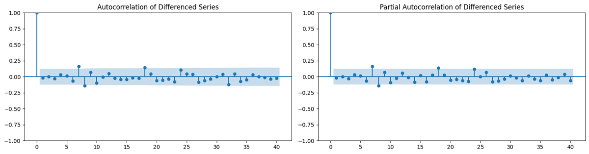
Figure 2: ACF and PACF plots used to determine optimal ARIMA hyperparameters. The ACF helps identify the order of MA terms, while the PACF helps select AR terms.

To ensure best-fitted parameters, the differenced data was graphically represented through an autocorrelation function (ACF) and partial autocorrelation function (PACF), which display the correlation of a time series with itself at different lags.
As Figure 2 shows, the ACF and PACF graphs both show spikes at the first few lags, after which a quick drop to 0, concluding that our ARIMA model will be particularly effective with low p and q values, which is how we have optimized the model.

Table 5 shows a comparison between the root mean squared error (RMSE), mean absolute error (MAE), and coefficients of determination of unoptimized parameters (p=1, d=1, q=1) and the optimized parameters (p=1, d=2, q=0). RMSE measures the square root of the average squared differences between predicted and actual values, penalizing larger errors more than smaller ones. MAE is less sensitive to outliers than RMSE, as it calculates the average absolute differences between predicted and actual values.

The following are the formulae of MAE and RMSE, respectively (Equations 4 & 5):

(4) $\begin{equation*}\text{MAE} = \frac{1}{n} \sum_{i=1}^{n} \lvert y_i - x_i \rvert\end{equation*}$

(5) $\begin{equation*}\text{MSE} = \sqrt{\frac{1}{n} \sum_{i=1}^{n} \left( y_i - x_i \right)^2 }\end{equation*}$

Here:

$y_i$ represents the predicted value
$x_i$ represents the actual value
$n$ represents the total number of data points

Model	RMSE	MAE
ARIMA(1, 1, 1) – Not optimized	268.26	268.11
ARIMA(1, 2, 0) – Optimized	162.66	140.96

Table 5

From the results shown in Table 5, it is evident that there is a significant decrease in both the RMSE and MAE post-optimization of the parameters, indicating better accuracy and reduced errors.

In conclusion, ARIMA is a particularly effective model when the data is stationary, as it models the relationship between past values and errors. However, this assumption of linearity limits its ability to capture other non-linear and seasonal patterns in the data and necessitates additional preprocessing. Despite these limitations, ARIMA was chosen for its ability to handle linear trends, simplicity, and effectiveness as a baseline model, allowing a comparison in performance to more advanced models like XGBoost Regressors and LSTM.

XGBoost Regressors

Extreme Gradient Boosting (XGBoost) is a machine-learning algorithm based on decision trees that has proven to be highly effective for regression, classification, and time series forecasting. XGBoost sequentially trains a collection of decision trees wherein each new tree attempts to correct the errors made by the previous one. Furthermore, XGBoost has built-in regularization that improves model generalization, and it optimizes a differentiable loss function through gradient descent.

The primary function of XGBoost is to minimize the objective function. The objective function consists of a loss term and a regularization term. The loss term represented by L is a loss function like the mean squared error between the actual value $y_i$ and predicted value $p_i$ . Additionally, K represents the number of trees and $\Omega (f_k)$ is the regularization term for each function $f_k$ .

The following function is the general formula of an objective function used in XGBoost regressors:

(6) $\begin{equation*}L(\theta) = \sum_{i=1}^{N} L(y_i, p_i) + \Omega(\theta)\end{equation*}$

The regularization term exists to penalize the complexity of the model and prevent overfitting by adding a cost for having too many large parameters. It is typically defined as:

(7) $\begin{equation*}\Omega(\theta) = \gamma T + \tfrac{1}{2} \lambda \sum_{j=1}^{T} w_j^2\end{equation*}$

Variables in Equations 6 and 7:

T is the number of leaves or nodes in the tree.
$\gamma$ is the hyperparameter that controls the penalty for adding more leaves or nodes in a tree. The larger this hyperparameter is, the more the model is penalized for having an excess of leaves, meaning that the model is encouraged to keep T small, leading to simpler trees.
$w_j$ is the weight of the jth leaf
$\lambda$ is a regularization hyperparameter that controls the size of the weights $w_j$ . A larger $\lambda$ value discourages large leaf weights, which prevents overfitting by discouraging complex leaf structures that have larger weights that might model noise.

In our implementation, XGBoost was configured with 100 estimators, max_depth=3, learning_rate=0.1, and incorporated lagged features for up to 4 time steps.

In conclusion, XGBoost is a powerful model that excels at capturing non-linear relationships and performing well on complex datasets. Its ability to incorporate various types of input data, including sentiment analysis, makes it ideal for predicting stocks in hybrid models. Despite being computationally intensive and requiring careful tuning to avoid overfitting, XGBoost was chosen for its superior predictive performance, particularly in handling large datasets with diverse features.

LSTM

Long Short-Term Memory (LSTM) is a type of recurrent neural network (RNN) that is designed to model sequential data, making it particularly well-suited for time series forecasting. It can capture both short-term and long-term dependencies in the data, overcoming the vanishing gradient problem in other RNNs. Unlike other classical models like ARIMA or XGBoost, LSTM is a deep learning model that automatically identifies complex patterns in sequential data without the need for extensive feature engineering or optimization. Due to these reasons, LSTM has generally outperformed other time series models for stock return predictions²

The vanishing gradient problem occurs when gradients become exponentially small during backpropagation, preventing effective learning in deep networks. One prominent challenge of deep learning models with several layers is the vanishing gradient problem, which occurs due to the sigmoid and hyperbolic tangent functions as their derivatives fall between 0 and 0.25, and 0 and 1, respectively. This leads to extreme weights becoming small, consequently causing the updated weights to resemble the original ones. However, LSTM overcomes the vanishing gradient problem by using three gates that regulate the flow of information, namely the forget, input, and output gates.

The following equations are of the different gates coupled with the hidden state:

(8) $\begin{equation*}f_t = \sigma \big( W_f \cdot [h_{t-1}, x_t] + b_f \big)\end{equation*}$

(9) $\begin{equation*}i_t = \sigma \big( W_i \cdot [h_{t-1}, x_t] + b_i \big)\end{equation*}$

(10) $\begin{equation*}o_t = \sigma \big( W_o \cdot [h_{t-1}, x_t] + b_o \big)\end{equation*}$

(11) $\begin{equation*}h_t = o_t \cdot \tanh(C_t)\end{equation*}$

Variables in Equations 8, 9, 10:

$W_f,W_i,W_o$ are the weight matrices for gates.
$x_t$ represents the input data at time step t.
$h_{t-1}$ represents the previous hidden state.
$\sigma$ is the sigmoid activation function, which outputs a value between 0 and 1.
tan⁡(h) is a hyperbolic tangent function that outputs a value between -1 and 1.
$b_f,b_i,b_o$ represent the bias terms for each gate
$C_t$ represents the memory cell state at time t

For our study, the LSTM network was configured with two layers (32 and 16 units), sequence length of 10 time steps, and trained for 50 epochs. In conclusion, LSTM is one of the few deep learning models that solves the vanishing gradient problem through its gating mechanisms, enabling it to capture both short- and long-term dependencies in the time series data, which is why it was chosen.

Results & Discussion

Before combining the sentiment analysis and time series models, it is necessary to incorporate various technical indicators (mathematical calculations based on historical price and volume data) to gain a broader understanding of market trends. These include the 7-day and 20-day moving averages (MAs), which are average prices over specified time periods; as well as the exponential moving averages (EMAs), which are weighted averages giving more importance to recent prices. The 7-day and 20-day moving averages were selected based on established literature in the field of technical analysis, because they fall within the established timeframes for identifying short-term trends and the momentum of a stock, respectively²³’²⁴. EMAs help smooth out short-term fluctuations and place greater weight on more recent data, allowing for better identification of long-term trends.

To combine the different models that have been used together, numerous feature sets were created by combining the sentiment from either VADER or Zero Shot Text Classification with each of the three distinct time series models, measuring RMSE and MAE to evaluate the impact that sentiment analysis has on traditional time series models.

The feature set includes solely the adjusted close prices as a baseline to measure the impact of adding sentiment scores, along with combinations of adjusted close prices and sentiment scores derived through various methods. For “Positive LLM,” tweets classified as positive about the stock were identified using Zero-Shot Text Classification, capturing the influence of positive sentiment.

Similarly, “Neutral LLM” and “Negative LLM” were created by extracting scores for neutral and negative classifications, respectively, using the same model. For “Positive VADER,” “Neutral VADER,” and “Negative VADER,” scores were automatically assigned by VADER for each analyzed text, requiring no additional classification steps. These combinations allow for a comprehensive analysis of the role of sentiment across different methods in stock price forecasting.

The weighting scheme in equations 12-14 follows established principles in behavioral finance where extreme sentiment signals carry more predictive information than neutral classifications. This approach aligns with prospect theory, which categorically shows that investors exhibit stronger reactions to clearly positive or negative information compared to ambiguous signals²⁵’²⁶. Other studies have attributed this because extreme sentiment events trigger disproportionate investor responses, with losses having an even greater emotional impact than equivalent gains²⁷. Recent behavioral finance research confirms that investors overreact to both positive and negative news while showing minimal response to neutral information, validating our emphasis on extreme sentiment values over neutral classifications²⁸’²⁹. Sentiment scores convert the multi-class output of the sentiment analysis models into unified numerical values that can be integrated as features in stock price prediction models. These scores aggregate positive, neutral, and negative classification probabilities into a single metric that quantifies the overall emotional tone of the tweet. These scores are calculated as a weighted combination of positive, neutral, and negative scores with the following formulae

(12) $\begin{equation*}S = \frac{1}{3} + \frac{2}{3}P \quad \text{if } P \geq N \text{ and } P \geq Ne\end{equation*}$

(13) $\begin{equation*}S= -1/3-N if N\ge P and N\ge Ne\end{equation*}$

(14) $\begin{equation*}S=P-N\end{equation*}$

otherwise (neutral is greater than both or balanced cases)

Variables in Equations 12, 13, 14:

S denotes the sentiment score.
P denotes the positive score
Ne denotes the neutral score
N denotes the negative score

The weighting parameters were designed to optimize the signal-to-noise ratio in sentiment classification. Strong sentiment signals (positive/negative) inherently carry more predictive information than neutral classifications, which often represent ambiguous or low-confidence predictions. This weighing scheme therefore amplifies extreme sentiment values while minimizing neutral ones, ensuring that the composite sentiment score reflects the most informative aspects of the classification output. This approach prevents neutral sentiment from diluting the signal when clear positive or negative sentiment is present.

Model Performance Analysis

These sentiment scores were then integrated as additional features in the machine learning models alongside traditional financial indicators. As shown in the feature sets, models receive both the adjusted closing price and the calculated sentiment score as input variables. For multivariate models like XGBoost and LSTM, sentiment scores are treated as lagged features (up to 4 lags) and processed through the same gradient boosting framework or neural network as the price data. This approach allows models to learn the correlation between sentiment signals and price movements, with the weighted sentiment formula ensuring that strong emotional signals (positive or negative) receive emphasis while neutral sentiment provides minimal influence.

The following Table (Table 6) displays the RMSE for all the feature sets for TSLA, which shows a significant increase in accuracy upon adding the sentiment scores.

Feature Set (TSLA)	RMSE of ARIMA	RMSE of XGBoost	RMSE of LSTM
Adj Close	40.59	1.07	12.06
Adj Close, Positive LLM	19.65	1.05	15.83
Adj Close, Positive VADER	20.41	1.074	15.26
Adj Close, Neutral LLM	21.41	1.069	14.42
Adj Close, Neutral VADER	20.94	1.071	13.25
Adj Close, Negative LLM	18.31	1.07	14.64
Adj Close, Negative VADER	20.32	1.07	11.37
Adj Close, Sentiment Score LLM	17.41	1.063	11.21
Adj Close, Sentiment Score VADER	20.45	1.067	14.3

Table 6

Bold values indicate best performance per model. Percentage improvements represent the proportional decrease in prediction errors when sentiment features are added compared to using stock prices alone.

For this analysis, we consider RMSE improvements >5% as meaningful, while improvements >20% are considered substantial.

The results from Table 6 highlight that sentiment analysis can significantly enhance predictive accuracy for stocks with high levels of public discourse, such as TSLA. The ARIMA model demonstrated the most substantial improvement, with the RMSE decreasing from 40.59 to 17.41 when incorporating sentiment scores derived from Zero-Shot Text Classification, representing a remarkable 57.1% improvement. Similarly, ARIMA integrated with VADER reduced the RMSE from 40.59 to 20.45, a 49.6% improvement.

Although the improvements in predictive accuracy for XGBoost and LSTM were less pronounced, there was still a slight reduction in RMSE for both models when incorporating sentiment scores. For instance, the RMSE of XGBoost decreased from 1.07 to 1.063, a minor 0.655% improvement, while the RMSE of LSTM decreased from 12.06 to 11.21, a sizeable 7.05% improvement. This suggests that while sentiment analysis has a more profound impact on simpler time series models like ARIMA, it still provides minor benefits to more complex models like XGBoost and LSTM, given that there is an adequate amount of sentiment volume.

While ARIMA’s absolute RMSE remains higher than that of the other models, the relative improvement indicates it still benefits from an integration with sentiment analysis.

Table 7 displays the RMSE for all the feature sets for AAPL, which shows both an increase in the accuracy of ARIMA, but also shows a decrease in the accuracy of XGBoost and LSTM upon adding the sentiment scores.

Feature Set (AAPL)	RMSE of ARIMA	RMSE of XGBoost	RMSE of LSTM
Adj Close	31.18	0.805	3.76
Adj Close, Positive LLM	9.11	0.800	3.44
Adj Close, Positive VADER	9.23	0.801	5.15
Adj Close, Neutral LLM	9.20	0.805	4.64
Adj Close, Neutral VADER	9.16	0.802	4.27
Adj Close, Negative LLM	9.07	0.809	4.36
Adj Close, Negative VADER	10.02	0.81	4.74
Adj Close, Sentiment Score LLM	9.08	0.81	4.62
Adj Close, Sentiment Score VADER	9.48	0.81	4.02

Table 7

The results from Table 7 indicate that sentiment analysis has a noticeable impact on the predictive accuracy of the ARIMA model for AAPL, though it decreases the accuracy for other models such as XGBoost and LSTM. For ARIMA, incorporating the sentiment scores derived from Zero-Shot Text Classification reduced the RMSE from 31.18 to 9.11, an unexpected 70.8% improvement.

In contrast, the impact of sentiment analysis on XGBoost and LSTM was negative. Despite XGBoost’s RMSE remaining stable across all feature sets, hovering around 0.80, it increased to 0.81 upon adding the sentiment scores of both VADER and Zero-Shot Text Classification. This suggests that XGBoost, with its ability to capture complex, non-linear patterns in the data, treats the sentiment scores as irrelevant noise. This leads to a decrease in predictive accuracy, preventing the model from achieving its highest potential. For LSTM, the results were more nuanced. While the RMSE for Zero-Shot Text Classification sentiment features was higher than that for VADER (4.62 vs. 4.02), this suggests an inverse correlation between the accuracy of sentiment extraction and its impact on LSTM’s predictive performance. In other words, more accurate sentiment scores from LLMs appear to be misleading to LSTM, perhaps due to the added complexity or misalignment between sentiment and stock price movements, leading to an overall decrease in model accuracy.

For a stock with a moderate number of tweets like AAPL, sentiment analysis can have both positive and negative impacts on predictive accuracy. While incorporating the sentiment scores significantly improved the performance of simpler models like ARIMA, their effect on more complex models such as XGBoost and LSTM was negative. These results highlight the critical role that the volume of public sentiment plays in the effectiveness of sentiment analysis. Stocks with higher public discourse, like TSLA, provide more reliable sentiment signals, which can enhance model predictions, whereas those with moderate levels of discourse may lead to more ambiguous or misleading results, especially for more sophisticated models. Table 8 displays the RMSE for all the feature sets for F, which shows a significant decrease in accuracy upon adding the sentiment scores:

Feature Set (F)	RMSE of ARIMA	RMSE of XGBoost	RMSE of LSTM
Adj Close	5.54	0.87	1.43
Adj Close, Positive LLM	5.87	0.87	1.91
Adj Close, Positive VADER	10.47	0.87	1.80
Adj Close, Neutral LLM	6.06	0.87	1.04
Adj Close, Neutral VADER	7.91	0.87	1.38
Adj Close, Negative LLM	7.27	0.87	0.78
Adj Close, Negative VADER	7.46	0.87	1.58
Adj Close, Sentiment Score LLM	5.41	0.87	2.023
Adj Close, Sentiment Score VADER	7.49	0.87	1.419

Table 8

Building upon the analysis of Apple (AAPL), the results for Ford (F) shown in Table 8 further emphasize the importance of the volume of public sentiment on the effectiveness of sentiment analysis. For ARIMA, the RMSE decreased from 5.54 to 5.41 when adding sentiment scores derived from Zero-Shot Text Classification, representing a minor improvement. However, this is a far smaller improvement compared to the more substantial gains observed for both TSLA and AAPL, indicating that no matter how accurate the models used for sentiment analysis are, a moderate volume is at least required for significant improvements in model performance. Furthermore, upon adding sentiment scores derived from VADER, it resulted in a slight increase in RMSE, from 5.54 to 7.49, indicating that inaccuracy in sentiment analysis when there is already a scarce amount of sentiment data is detrimental for the overarching accuracy of the model.

In the same vein, Zero-Shot Text Classification consistently outperformed VADER across the other stocks, indicating that the sentiment analysis method chosen and its accuracy are crucial. Transformer-based models like Zero-Shot Text Classification excel in capturing context, nuance, and even sarcasm in tweets, resulting in more accurate sentiment extraction. Consequently, these sentiment features significantly improve predictive performance, particularly for models such as ARIMA, XGBoost, and LSTM when applied to high-discourse stocks.

For XGBoost, there were no significant changes in RMSE in all feature sets, likely because the volume of sentiment was so low that the noise was not large enough in volume to change the accuracy, whereas in the case of AAPL, the amount of public discourse was greater, therefore reducing the accuracy of XGBoost. This also supports our hypothesis, which states that sentiment analysis is most useful for stocks with high public discourse. Likewise, the inverse relationship between the accuracy of tweets analyzed in sentiment analysis and the performance of LSTM persists.

Furthermore, the mathematical integration of sentiment scores as additional features demonstrates that the effectiveness of sentiment analysis depends critically on discourse volume. For high-discourse stocks like TSLA, the lagged sentiment features provide meaningful predictive signals that enhance model accuracy, with XGBoost and LSTM able to learn complex relationships between sentiment patterns and price movements. However, for low-discourse stocks, sparse sentiment data introduces noise that degrades performance, particularly in simpler models like ARIMA that treat sentiment linearly.

Feature Correlation

To understand feature relationships for our models, we examined correlations between sentiment features and adjusted closing prices across all three stocks.

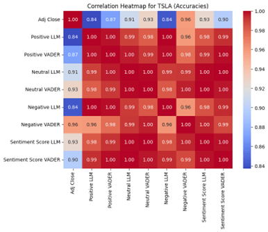
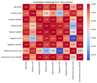
Figure 3 presents correlation heatmaps that reveal distinct patterns across discourse levels that explain our model performance differences. For Tesla (Figure 3a), sentiment features show meaningful differentiation in their relationships with adjusted close prices. Positive LLM correlates at 0.84, Negative LLM at 0.84, while Positive VADER shows 0.87 and Negative VADER at 0.96. This variation in correlation coefficients, ranging from 0.84 to 0.96, shows that different sentiment features capture distinct aspects of market behavior. The diversity in these correlations means each feature provides unique information to the models, which allows them to learn different patterns and relationships, resulting in substantial accuracy improvements as the varied correlation patterns enable the models to extract complementary signals from multiple dimensions of sentiment.

For Apple (Figure 3b), correlations show reduced differentiation than Tesla, as the correlations are clustered from the range of 0.92 to 0.97. This smaller variation in correlation coefficients limits the unique information each sentiment feature can provide, resulting in more modest accuracy improvements compared to Tesla. It also explains why Apple shows smaller improvements from sentiment analysis.

For Ford (Figure 3c), correlations cluster tightly around 0.97 – 1.00 across all sentiment features. Unlike the other stocks, Positive LLM, Positive VADER, Negative LLM, and Negative VADER all show nearly identical correlations with adjusted close prices. This uniformity in the correlations indicates that a sparse volume of tweets fails to generate meaningful sentiment differentiation. These near-perfect correlations suggest the sentiment features are essentially capturing the same underlying price patterns rather than independent sentiment signals, meaning they become redundant with the price data itself. This redundancy explains why our models show either minimal increases or even slight decreases in accuracy for Ford, caused by the sentiment features mirroring the stock price data too closely, which creates noise rather than a signal and confuses the models that expect independent predictive information. This inevitably leads to overfitting on false correlations.

Furthermore, Ford’s sentiment analysis may be unreliable due to extremely low tweet volume (31 tweets across a year). This scarcity of public sentiment implies that several trading days would lack any sentiment data, which would lead to noise propagation, meaning that all sentiment-derived predictions for Ford should be interpreted cautiously.

The correlation heatmaps confirm our hypothesis, as they show that a high volume of discourse enables diverse sentiment signals that enhance prediction, while low volumes of discourse produce redundant signals that do not offer any predictive advantage.

Confounding Variables

Several external factors beyond just sentiment could have influenced the results during the time in which the study was conducted (September 2021 to September 2022). This is because the timeframe chosen included major events such as changes in the Federal Reserve’s interest rate, concerns about inflation, the long-term impact of COVID-19, which still impacted markets, and the acquisition of Twitter by Elon Musk. For Tesla specifically, its CEO, Elon Musk’s tweets and business announcements create a unique externality, in which his statements can instantly affect both general public sentiment and stock prices, making it difficult to distinguish between cause and effect.

While no study can fully isolate the effects of sentiment analysis from these systematic confounding variables, the differential performances across low, moderate, and high discourse stocks suggest that sentiment volume itself plays a notable role beyond these confounding factors.

Additionally, our study lacks comparison with modern and established baseline methods in financial sentiment analysis and stock prediction. These industry-standard approaches, including analyst consensus forecasts, traditional econometric models, or established sentiment analysis benchmarks, would provide more information to critically evaluate the performance of the models. The lack of these comparisons limits our ability to make a generalized conclusion of our findings relative to existing market prediction methods.

Conclusion

This study demonstrates that sentiment analysis can significantly enhance the accuracy of stock price predictions, but its effectiveness relies on the level of public discourse surrounding the stock. For stocks like TSLA, which have tens of thousands of Tweets about them in one single year, sentiment features derived from Zero-Shot Text Classification led to a substantial 57.1% improvement in ARIMA’s accuracy and a considerable 21.6% average improvement in accuracy for the three models. This validates the hypothesis that sentiment analysis is most beneficial when the volume of public sentiment is high. On the other hand, for stocks with less than 1000 tweets, like Ford, the impact of sentiment analysis was negligible, even detrimental for some models, which highlights the limitations and reliability of sentiment analysis when used for smaller stocks.

Furthermore, this study also emphasizes the importance of model choice, while ARIMA showed the most improvements due to the addition of sentiment analysis, XGBoost consistently had the highest accuracy due to its ability to capture complex and nonlinear trends in the dataset. This underscores the need for careful integration of sentiment analysis, particularly for complex models like LSTM, which may struggle with nuanced inputs from advanced sentiment models. Not to mention that the model used to conduct sentiment analysis is also vital for accuracy, as Zero-Shot Text Classification consistently outperformed VADER due to its transformer architecture and ability to understand context and nuances within tweets.

These findings have significant implications for financial forecasting. They suggest that hybrid models combining sentiment analysis and market data are most effective for stocks with high levels of public attention, wherein the public discourse provides meaningful signals. However, for stocks with limited public sentiment, traditional quantitative models will remain more stable.

Nevertheless, this study is not without limitations; the reliance on tweets as a measure of public sentiment is incomplete as it excludes other sources like news articles and broader public forums. Additionally, the analysis was limited to three stocks over a one-year period (2021-2022), which may not capture the full spectrum of market dynamics across different sectors and time periods. Specifically, this one-year period analysis raises concerns about potential overfitting to specific market conditions or temporal bias, as the models were not trained or validated across different market cycles or economic environments, which limits our ability to deduce general rules or trends observed as they may not apply to varying markets.

In the same vein, this study focuses on next-day predictions only, without exploring long-term forecasting accuracy, lag effects of sentiment, or cross-validation across different time periods. This limits our insight into the long-term effects of sentiment. Future research should explore multi-horizon forecasting to understand the persistence of sentiment and patterns over longer time periods than one day. Furthermore, future research could also expand the dataset to include more diverse stocks and explore alternative sentiment sources such as news articles, public forums, or other social media applications. Moreover, future research should also consider exploring other dynamics of sentiment, such as momentum or decay, as it would provide deeper insights into how these factors impact the predictive accuracy of the models.

From an ethical perspective, this research raises important ethical issues, most notably regarding the enabling of market manipulation through sentiment analysis, particularly due to the prevalence of automated bot accounts on social media. Not to mention that using social media content for financial predictions raises data privacy issues. Lastly, sentiment-based trading systems create unfair advantages for individuals and institutions with advanced analytics capabilities that can capture large amounts of public sentiment over retail investors. This stark inequality could contribute to market instability.

Additionally, developing adaptive models that automatically weight or filter sentiment features appropriately based on the volume of public discourse available thresholds could optimize performance across stocks with varying levels of public attention.

The implementation of the models and the dataset is publicly available in the following GitHub Repository: https://github.com/nigamanthsrivatsan/HybridStockForecasting

In conclusion, the study contributes to the understanding of how sentiment analysis interacts with traditional forecasting models, providing a framework for combining qualitative and quantitative data in financial prediction. Demonstrating the importance of public discourse volume and model selection paves the way for more nuanced approaches to market forecasting.

Abbreviations

NLP: Natural Language Processing
VADER: Valence Aware Dictionary and sEntiment Reasoner
LLM: Large Language Models
MLM: Masked Language Modeling
ARIMA: AutoRegressive Integrated Moving Average
AR: AutoRegressive
MA: Moving Average
EMA: Exponential Moving Average
ADF: Augmented Dickey-Fuller
RMSE: Root Mean Squared Error
MAE: Mean Absolute Error
LSTM: Long Short-Term Memory
RNN: Recurrent Neural Network
XGBoost: Extreme Gradient Boosting
AI: Artificial Intelligence

References

Broby D. The use of predictive analytics in finance. J Finance Data Sci, 8: 145-161, 2022. [↩]
Fischer T, Krauss C. Deep learning with long short-term memory networks for financial market predictions. Eur J Oper Res, 270(2): 654-669, 2018. [↩] [↩]
Shiller RJ. Measuring bubble expectations and investor confidence. J Psychol Financ Mark, 1(1): 49-60, 2000. [↩]
Bollen J, Mao H, Zeng X. Twitter mood predicts the stock market. J Comput Sci, 2(1): 1-8, 2011. [↩]
Li X, Xie H, Chen L, Wang J, Deng X. News impact on stock price return via sentiment analysis. Knowl-Based Syst, 69: 14-23, 2014. [↩]
Loughran T, McDonald B. When is a liability not a liability? Textual analysis, dictionaries, and 10-Ks. J Finance, 66(1): 35-65, 2011. [↩]
Araci D. FinBERT: Financial sentiment analysis with pre-trained language models. arXiv preprint, arXiv:1908.10063, 2019. [↩]
Jing N, Wu Z, Wang H. A hybrid model integrating deep learning with investor sentiment analysis for stock price prediction. Expert Syst Appl, 178: 115019, 2021. [↩]
Li Y, Pan Y. A novel ensemble method for stock prediction based on multi-view heterogeneous data. Financial Innovation, 9(1): 89, 2023. [↩]
Ranco G, Aleksovski D, Caldarelli G, Grčar M, Mozetič I. The effects of Twitter sentiment on stock price returns. PLoS One, 10(9): e0138441, 2015. [↩]
Cookson JA, Niessner M. Why don’t we agree? Evidence from a social network of investors. J Finance, 75(1): 173-228, 2020. [↩]
Jiang W, Zeng J. Predicting stock prices with FinBERT-LSTM: integrating news sentiment analysis. Proc 8th Int Conf Cloud Big Data Computing, 234-241, 2024. [↩]
Fatemi B, Hu J. A comparative analysis of fine-tuned LLMs and few-shot learning of LLMs for financial sentiment analysis. arXiv preprint, arXiv:2312.08725, 2023. [↩]
Hutto CJ, Gilbert E. VADER: A parsimonious rule-based model for sentiment analysis of social media text. Proc Int AAAI Conf Web Social Media, 8(1): 216-225, 2014. [↩]
Yin W, Hay J, Roth D. Benchmarking zero-shot text classification: Datasets, evaluation and entailment approach. Proc Conf Empirical Methods Natural Language Process, 3914-3923, 2019. [↩]
Krippendorff K. Content Analysis: An Introduction to Its Methodology. 3rd ed. Thousand Oaks, CA: SAGE Publications; 2012. [↩] [↩]
Malo P, Sinha A, Korhonen P, Wallenius J, Takala P. Good debt or bad debt: Detecting semantic orientations in economic texts. J Assoc Inf Sci Technol, 65(4): 782-796, 2014. [↩] [↩]
Boukes M, Welbers K, Tsuboki L, van Atteveldt W. The validity of sentiment analysis: Comparing manual annotation, crowd-coding, dictionary approaches, and machine learning algorithms. Mass Commun Soc, 24(2): 220-245, 2021. [↩]
Gonçalves P, Araújo M, Benevenuto F, Cha M. Comparing and combining sentiment analysis methods. Proc ACM Conf Online Soc Netw, 27-38, 2014. [↩]
Du L, Ding X, Li T, Zhang Y. Financial Sentiment Analysis: Techniques and Applications. ACM Comput Surv, 57(2): 1-42, 2024. [↩]
Smith A, Johnson B. BERT applications in financial sentiment analysis: A comprehensive review. J Mach Learn Finance, 12(3): 78-95, 2024. [↩]
Chen W, Liu M, Wang K. Financial Sentiment Analysis and Classification. MDPI Appl Sci, 15(4): 1823, 2025. [↩]
Murphy JJ. Technical Analysis of the Financial Markets: A Comprehensive Guide to Trading Methods and Applications. New York Institute of Finance, New York, NY, 1999. [↩]
Brock W, Lakonishok J, LeBaron B. Simple technical trading rules and the stochastic properties of stock returns. J Finance, 47(5): 1731-1764, 1992. [↩]
Kahneman D, Tversky A. Prospect theory: an analysis of decision under risk. Econometrica, 47(2): 263-291, 1979. [↩]
Daniel K, Hirshleifer D, Subrahmanyam A. Investor psychology and security market under- and overreactions. J Finance, 53(6): 1839-1885, 1998. [↩]
Tversky A, Kahneman D. Loss aversion in riskless choice: a reference-dependent model. Q J Econ, 106(4): 1039-1061, 1991. [↩]
Mian GM, Sankaraguruswamy S. Investor sentiment and stock market response to earnings news. Account Rev, 87(4): 1357-1384, 2012. [↩]
Piccoli P, Chaudhury M. Overreaction to extreme market events and investor sentiment. Appl Econ Lett, 25(2): 115-118, 2018. [↩]

Using Large Language Models to Predict Stock Price: A Hybrid Model Combining Social Media Sentiment and Market Data

Abstract

Introduction

Methods

Data Preprocessing & Exploratory Data Analysis