United We Predict: An Ensemble Learning Approach to Unmask Fake News

Abstract

The spread of fake news presents a significant challenge to society necessitating accurate detection systems. This study explores the application of an ensemble learning approach for fake news detection. The approach relies on combining the embeddings of Bidirectional Encoder Representations from Transformers (BERT) , Robust Bidirectional Encoder Representations from Transformers (RoBERTa) and Bi-directional Long Short-Term Memory (BiLSTM) into a single feature vector. Subsequently, the light gradient boosting machine (LightGBM) classifier identifies the best combination of embeddings from the combined feature vector for predicting truthfulness using six classes. Utilizing the LIAR dataset, the proposed ensemble learning approach is benchmarked against stand-alone deep learning and recurrent neural network models. The results demonstrate that the ensemble learning model achieves modestly effective performance (accuracy= 0.40, F1 score= 0.40) compared to stand-alone models (accuracy of BERT= 0.26, accuracy of RoBERTa =0.20, accuracy of BiLSTM=0.20, accuracy of LSTM=0.19) making it a viable solution for fake news detection. This study contributes to the limited body of research that uses LightGBM in conjunction with transformer-based and neural network models for misinformation detection. Future work will focus on incorporating speaker metadata to assess performance improvement and assessing whether feature importance analysis from the LightGBM can help in reducing the number of dimensions and streamlining the model.

Keywords: Fake News, Ensemble Learning, BERT, RoBERTa, BiLSTM, Gradient Boosting Machine

Introduction

The rapid spread of misinformation on social media platforms poses significant threats to public discourse and democratic processes1,¹. The danger of misinformation lies in the fact that the public tends to believe it initially and attempts to rectify it later proves to be expensive3. While traditional fact-checking relies on human experts, the quick speed at which misinformation spreads necessitate automated detection systems. Current approaches to fake news detection employ either deep learning models or traditional machine learning classifiers, each with distinct limitations. Deep learning models, particularly transformer-based architectures like Bidirectional Encoder Representations from Transformers (BERT) and Robust Bidirectional Encoder Representations from Transformers (RoBERTa), demonstrate superior semantic understanding but require substantial computational resources and training time4,². Conversely, traditional machine learning approaches offer computational efficiency but often lack the semantic depth necessary for nuanced misinformation detection6. Fake news detection presents additional challenges as statements often fall along a spectrum of truthfulness rather than binary true/false categories. The LIAR dataset, with its six classes of truthfulness exemplifies the range of misinformation that is seen in political statements.

Research Contributions

This study addresses the critical need for a scalable and accurate fake news detection systems. The study’s primary contributions are: (1) a development of a hybrid ensemble model that combines feature extraction from multiple deep learning models with lightweight gradient boosting machine (LightGBM) classification and (2) a demonstration that ensemble feature fusion can achieve competitive performance compared to individual deep learning models.

Literature Review

In this section, related research on the use of ensemble learning models for detecting fake news is reviewed. Hansrajh, Adeliyi and Wing developed a blending ensemble machine learning approach for automated fake news detection³. The study developed a system that combines five base machine learning algorithms (logistic regression, support vector machine, linear discriminant analysis, stochastic gradient descent, and ridge regression) using natural language processing techniques including Term Frequency-Inverse Document Frequency (TF-IDF) and n-grams for feature extraction. The blending ensemble model outperformed individual classifiers, achieving 60.81% accuracy on the Liar dataset. However, the study did a binary classification of truth, converting the original six-category labels from the datasets into simple “true” or “fake” classifications.

Essa, Omar and Alqahtani proposed a hybrid fake news detection system combining BERT with LightGBM⁴. Their method uses BERT as a feature extractor to generate contextualized word embeddings by concatenating the classification [CLS] token representations from the last three hidden layers, which are then fed into a LightGBM classifier for final prediction. The system was evaluated on three real-world datasets (ISOT with 45,000 articles, TI-CNN with 20,015 articles, and FNC with 1,000,000 articles) and compared against machine learning approaches using TF-IDF and Global Vectors (GloVe) embeddings with classifiers like Multinomial Naive Bayes, Linear Regression, Support Vector Machine (SVM), and Long Short-term Memory (LSTM). The hybrid BERT-LightGBM model achieved superior performance with accuracies of 99.88% on ISOT, 96.94% on TI-CNN, and 99.06% on FNC datasets, outperforming all baseline methods. This study also performed a binary classification of news articles as either “real” or “fake.”

Dev and coauthors developed a hybrid deep learning model that combines Convolutional Neural Networks (CNN) with LSTM networks⁵. Their methodology involved extensive text preprocessing using Natural Language Processing techniques, feature extraction through Count Vectorizer and TF-IDF Vectorizer from Python’s scikit-learn library, and the implementation of GloVe word embeddings to capture contextual relationships in the text. Testing on a Kaggle dataset containing 7,796 news articles with balanced fake and real content, their CNN+LSTM hybrid approach achieved 98% accuracy, outperforming individual models like standard neural networks (93%), recurrent neural networks (RNN) +LSTM (91%), and other baseline approaches including AdaBoost (97%), Logistic Regression (95%), and Artificial Neural Networks (93%). This study also classified the news articles as either “fake” or “real.”

Parthiban, Alex and Peter proposed an Integrated Hybrid Deep Learning AI (IHDLAI) framework to classify fake news as either “fake” or “real”⁶. The paper used a comprehensive three-phase approach combining multiple deep learning architectures to enhance fake news detection capabilities. Their methodology integrated Convolutional Neural Networks (CNNs) for capturing spatial patterns in textual data, RNNs with LSTM cells for sequential dependency analysis, and BERT models for contextual understanding, all combined through an ensemble voting mechanism. Testing on the LIAR dataset, their hybrid ensemble approach achieved 94% accuracy, 96% precision, 94% recall, and 94% F1-score, significantly outperforming individual models (CNN: 85%, RNN-LSTM: 87%, BERT: 92% accuracy).

Pillai developed a multi-class fake news detection approach using transformer models and gradient boosting on the LIAR dataset, categorizing news statements into six levels of truthfulness⁷. Using the LIAR dataset (10,269 training records, 1,284 validation, and 1,283 test records), their study found that the best-performing GBM ensemble achieved only 41% accuracy with an F1-score of 0.42, while individual models performed much worse (BERT: 22% accuracy, RoBERTa: 23%, BiLSTM: 21%). The study demonstrates that while ensemble methods can improve performance over individual models, the complexity of distinguishing between nuanced levels of truthfulness remains a significant challenge.

Yadav and coauthors developed a hybrid deep learning approach combining CNN and BiLSTM architectures with different word embedding techniques⁸. The paper again used binary classification of news articles as either “fake” or “real,”. The paper used two publicly available datasets (Fake and real news dataset with 44,919 articles and allData with 20,015 articles) to create a larger training dataset of 64,934 labeled news articles. After evaluating 16 different machine learning configurations and 12 deep learning model combinations, their best-performing model (CNN-BiLSTM with Word2Vec embeddings) achieved 97.5% accuracy, 98.4% precision, 97.0% recall, 97.7% F1-score, and 99.2% Area under the curve- Receiver Operating Characteristics (AUC-ROC), outperforming individual models like LSTM (94.4% accuracy), BiLSTM (97.0% accuracy), and traditional machine learning approaches such as SVM (92.3% accuracy).

Research Gap and Motivation

The literature review indicates two research gaps in fake news detection methodologies. First, while several studies have examined binary classification of fake news, studies examining six-class classification of fake news are very limited. Second, while previous studies have demonstrated the effectiveness of ensemble learning approaches for binary fake news classification, achieving impressive accuracies ranging from 60.81% to 99.88% across various datasets, a performance degradation is seen in the context of multi-class detection. A question that arises is whether current natural language processing techniques can capture the nuanced linguistic and contextual features to detect different levels of truthfulness. The motivation for this paper is to use an ensemble learning model for a six-class classification of fake news and add to the limited body of research that attempts to study this challenging problem. In addition, the study’s motivation is also to explore whether the performance of an ensemble learning model for six-class classification can be improved beyond what the study by Pillai documented⁷.

Methods

Dataset Description

The LIAR dataset is a publicly available resource comprising 12.8K manually labeled short statements from various contexts, such as political debates, TV ads, and social media posts. Each statement is annotated with one of six truthfulness ratings: true, mostly-true, half-true, barely-true, false and pants-fire. In addition to the statements, the dataset included metadata such as the subject, speaker, job title, state and party affiliation of the speaker.

Data Acquisition

The dataset was obtained from the official repository provided by the authors⁹. An automated script was developed to download and extract the dataset, ensuring reproducibility and efficiency in data handling. The script checks for the existence of the dataset locally to avoid unnecessary downloads and proceeds to download and unzip the dataset if not found.

To understand the characteristics of the LIAR dataset, Figure 1 presents the frequency count of the most frequently occurring topics among the labeled statements. Thematically, the dataset is dominated by politically relevant issues such as the economy, healthcare, and taxes, which often attract misinformation and public scrutiny. Approximately, a third of the political statements in the LIAR dataset feature topics related to the economy, healthcare and taxes. The possibility that these topics involve complex factual claims that often require verification, and policy knowledge is indicative of an inherent challenge in the LIAR dataset.

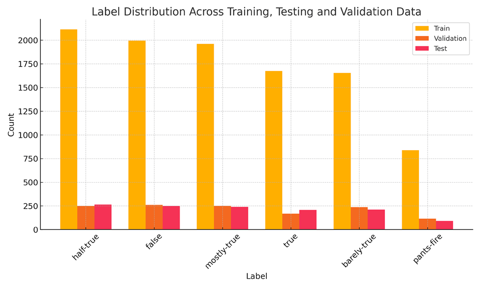
Figure 2 shows the distribution of the six truthfulness labels, “True,” “Mostly True,” “Half True,” “Barely True,” “False,” and “Pants on Fire”, across the training, validation, and test sets. The relatively balanced label distribution supports the use of accuracy and F1-score as performance metrics and confirms that the model was trained and tested on a representative set of statements. These distributions also highlight the challenges of the task, as categories such as “Pants on Fire” are under-represented in the dataset. The challenge is whether the model can learn effectively from a relatively smaller sample of “Pants on Fire” statements.

Data Preprocessing

The dataset was provided in tab-separated values (TSV) format and split into training, validation and test sets. The pandas library was used to read the TSV files into DataFrames for efficient data manipulation. The columns were renamed to meaningful names for better readability and ease of reference during data processing. The primary columns used in this study included:

• ID: Unique identifier for each statement
• Label: The truthfulness rating assigned to the statement
• Statement: The actual textual content of the statement

Label Encoding

The numerical labels y_i  were converted into one-hot encoded vectors y_i ∈ R⁶  where each vector has a value of 1 at the index corresponding to the label and 0 elsewhere

(1)  

(2)  

Data Splitting

The dataset was already partitioned into training, validation and test sets by the dataset authors (80% training, 10% validation and 10% testing) ensuring that the model’s performance could be evaluated on unseen data. The splits are as follows:

• Training Set: Used to train the model parameters
• Validation Set: Used for hyperparameter tuning and to prevent overfitting via early stopping
• Test Set: Used to assess the final performance of the model

Summary of Data Preparation Steps

The data preparation involved the following key steps:

• Data Acquisition: Automated downloading and extraction of the dataset
• Data Loading: Reading the TSV files into structured DataFrames
• Data Cleaning: Renaming columns and ensuring data integrity
• Feature Engineering: Computing statement lengths and transforming textual data into numerical feature vectors using the bag of words (BoW) model
• Label Encoding: Converting categorical labels into numerical and one-hot encoded formats
• Data Reshaping: Adjusting the shape of the data to match the input requirements of the transformer and BiLSTM models

These preprocessing steps ensure that the data was in an optimal format for training, facilitating efficient learning and improving the potential for accurate classification.

Method Layout and Rationale for Model Selection

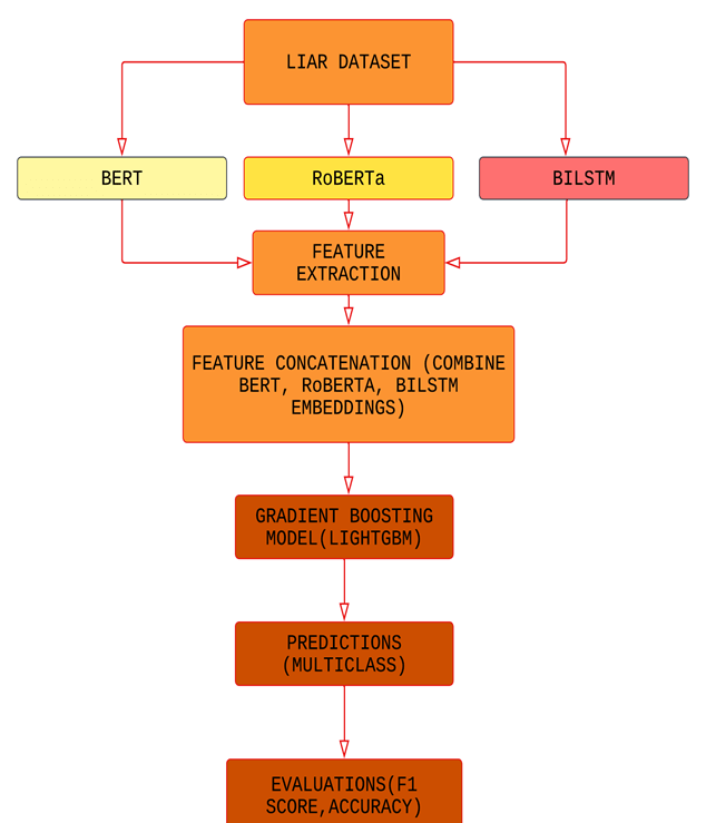
The proposed model employs a hybrid approach that combines deep learning and machine learning to classify fake news into six categories. The selection of BERT, RoBERTa, and BiLSTM as foundational models for feature extraction in the ensemble architecture is driven by their complementary strengths in capturing semantic, contextual, and sequential patterns in text, an essential requirement for accurately classifying fake news statements, which often rely on subtle phrasing, partial truths, or ambiguous claims. Figure 3 shows the layout of the proposed ensemble learning approach.

As figure 3 depicts, the system leverages multiple state-of-the-art natural language processing models for feature extraction. BERT (Bi-directional Encoder Representations from Transformers) and its optimized variant RoBERTa analyze text bidirectionally, capturing deep contextual relationships through transformer architectures, while BiLSTM (Bidirectional Long Short-Term Memory) processes text sequences in both forward and backward directions to better understand word order and local context¹⁰’²’¹¹. These models work in parallel, with BERT and RoBERTa extracting 768-dimensional embeddings from their [CLS] tokens and BiLSTM generating sequential representations of the text . As seen in figure 3, the features from BERT, RoBERTa and BiLSTM are concatenated before being fed to the GBM for multiclass predictions.

The hybrid architecture offers several advantages, including deep contextual understanding from BERT and RoBERTa, and sequential processing capabilities from BiLSTM. The advantage of using LightGBM as a final classifier is that it can learn patterns from the text embeddings (e.g., BERT, RoBERTa, BiLSTM outputs) and identify complex patterns in the high-dimensional feature space created by these embeddings. LightGBM does not generate features but instead it learns how to best combine the features to predict each truth class. Performance is evaluated using accuracy and F1-score to balance precision and recall, ensuring robust detection of both blatant and subtle misinformation. By combining these techniques, the model achieves improved classification performance compared to standalone approaches.

BERT Architecture

The BERT architecture utilizes a transformer-based approach with multiple bidirectional encoder layers. Each layer contains self-attention mechanisms that allow the model to weigh the importance of different words in a sentence. The input undergoes WordPiece tokenization before being processed through transformer layers, with each word’s representation informed by its context. A special [CLS] token aggregates sentence-level information for classification tasks. BERT’s strength lies in its pre-training on massive text corpora using masked language modeling, where it learns to predict randomly masked words in sentences¹².

BERT (Bidirectional Encoder Representations from Transformers) understands language by looking at all the words in a sentence at once, instead of just left-to-right or right-to-left. Each word in a sentence is first turned into a vector (a list of numbers) called an embedding, which includes both the meaning of the word and its position. BERT uses a method called self-attention, where every word compares itself to all other words in the sentence. Mathematically, this is done by computing similarity scores between word vectors using the formula¹³:

Attention(Q,K,V) = softmax ( (QK^T)/√d)V,

Q is the query matrix that represents the current word (or token)

K is the Key matrix that represents all words as “labels” that can be matched against queries.

T is the transpose operator

V is the Value matrix that represents the actual information carried by each word.

d is the dimensions of the key vectors that are used for scaling

softmax is a function that converts the scores into probabilities between 0 and 1

BERT is trained in two main ways. First, some words in a sentence are hidden and the model seeks to guess them (called Masked Language Modeling). Second, it predicts whether one sentence follows another (Next Sentence Prediction). By combining these training methods, BERT learns deep, bidirectional representations of language that can then be applied to many tasks such as classification of truthfulness in political statements.

RoBERTa Architecture

RoBERTa (Robustly Optimized BERT Pretraining Approach) is a model built on top of BERT, but with some important improvements in how it is trained. Like BERT, it represents each word as a vector and uses the self-attention formula Attention (Q,K,V) = softma x¹⁴’¹².

BiLSTM Architecture

Figure 5 depicts the architecture of the BiLSTM model. The BiLSTM architecture processes text sequentially in both forward and backward directions through specialized memory cells. Each LSTM unit contains gates that regulate information flow, enabling the network to learn long-range dependencies in text. The forward pass analyzes the sentence from start to end, while the backward pass processes it in reverse. As shown in figure 5, hidden states from both directions are concatenated at each timestep, providing a rich representation that captures contextual relationships from the entire sentence¹⁵’¹⁶. This bidirectional processing makes BiLSTM particularly effective for understanding word order and local linguistic patterns¹⁵’¹⁷. The dropout layer in figure 5 turns off a fraction of the neurons during training to make sure the model is not overfitting.

The following mathematical equations describe the operations of a Long Short-Term Memory (LSTM) unit at time step t. In a BiLSTM, these equations are applied in both forward and backward directions, and the final hidden state is formed by concatenating them¹⁸’¹⁶.

The model takes the current input and the previous hidden state , applies weights , adds a bias , and the sigmoid function outputs values between (completely forget) and (completely keep).

(input gate)

This is like the forget gate but controls what portion of new candidate memory gets added.
(output gate)

This acts like a “filter” on the memory cell contents before sending it to the next layer or prediction

(candidate memory)

This generates a set of new information that could be added to the cell state.

(cell state update)

This updates the memory cell by combining old information and new information. It is the core memory update that lets the LSTM remember things over long sequences.

(hidden state update)

This produces the output for this time step which is passed to the next step or used for predictions.

(bidirectional concatenation)

In a BiLSTM, the forward and backward hidden states are combined.

Feature Vector Construction

To prepare the input for classification, a unified feature vector was constructed that combines contextual information extracted from multiple deep learning models. Each news statement was independently processed by BERT, RoBERTa, and BiLSTM. BERT and RoBERTa each generated 768-dimensional sentence-level embeddings using their [CLS] tokens, while BiLSTM captured sequential dependencies by processing the input text in both forward and backward directions.

The resulting embeddings were then concatenated into a single feature vector, combining the semantic richness of transformer-based models with the sequential feature of BiLSTM¹⁹. Specifically, np.hstack was used to combine the feature vectors generated by BERT, RoBERTa, and BiLSTM into a single, unified vector. Each of these models captures different aspects of the input text such as semantic meaning, contextual relationships, and sequential patterns. By horizontally stacking (hstacking) their outputs, one comprehensive feature representation of each news statement was created¹⁹. This fused representation served as the input to the LightGBM classifier, enabling the model to make fine-grained predictions across six truthfulness categories. By relying solely on text-based features, the architecture is lightweight and adaptable to real-time classification tasks. LightGBM processes the mixed feature types, iteratively building decision trees to classify news statements into one of six categories: “True,” “Mostly true,” “Half true,” “Barely true,” “False,” or “Pants on fire” (completely false).

LightGBM Architecture

The LightGBM layout in the hybrid fake news detection system serves as the final classification stage, where it processes the combined feature vectors extracted from BERT, RoBERTa, and BiLSTM models. Figure 6 depicts the architecture of LightGBM. As shown in figure 6, LightGBM takes these pre-processed text embeddings as input, then applies its gradient-boosted decision tree algorithm to make the final classification. LightGBM (Light Gradient Boosting Machine) builds many small decision trees one after another, where each new tree tries to fix the mistakes of the previous ones. These are the residuals in Figure 6. Mathematically, suppose we want to predict a target y_i from input x_i. LightGBM builds a model as the sum of decision trees²⁰:

where each is a regression tree.

At each step, the model minimizes an objective function that includes both a loss term and a regularization term:

where is a loss function (similar to squared error in regression), and penalizes tree complexity²⁰.

The output layer produces one of six possible classification labels ranging from “True” to “Pants on Fire,” completing the end-to-end fake news detection pipeline. This layout emphasizes LightGBM’s role as an efficient aggregator of deep learning features for real-world deployment.

Hyperparameters tuning and regularization

During training, three separate BERT based models were trained, each for 3 epochs. After each epoch, the model was evaluated on the validation set and the training and validation accuracy was recorded. The model weights were saved after each epoch to preserve intermediate checkpoints and facilitate later analysis or ensemble methods.

An optimization approach was employed to fine-tune the hyperparameters in two stages. Initially, a random search was conducted to broadly explore the hyperparameter space, which helped identify promising regions for each model type. Following this initial exploration, Optuna, a hyperparameter optimization framework, was used to perform more targeted refinement within the identified promising regions, ensuring optimal performance across all model architectures²¹. The optimal learning rates discovered were 2e-5 for both BERT and BiLSTM models, 1.85e-05 for RoBERTa, and 0.05 for LightGBM. The dropout rate of 0.10 was applied to the BiLSTM model to prevent overfitting by randomly deactivating 10% of the neurons during training. This prevents the model from memorizing the training data based on a few specific neurons and forces it to learn generalizable patterns across many neurons. The dropout rate of 0.10 is a good middle ground as a higher dropout rate such as 0.30 can leave out many neurons and have the risk of the model underfitting. At the same time, a dropout rate of 0.05 can leave out too few neurons and have the risk of the model overfitting.

Results

Before discussing the model performance, it is crucial to understand the metrics used to assess its effectiveness in multi-class classification. This study relied on accuracy and F1-score, as they provide a comprehensive view of a model’s predictive capabilities, especially in scenarios where class distribution might be imbalanced.

• Accuracy: Accuracy is a fundamental metric that measures the proportion of correctly classified instances out of the total number of instances. It is calculated as:

Accuracy = Number of Correct Predictions /Total Number of Predictions​

While intuitive, accuracy can be misleading in datasets with significant class imbalance, as a model might achieve high accuracy by simply predicting the majority class.

• F1 score: The F1-Score is the harmonic mean of Precision and Recall, offering a more balanced evaluation, particularly useful in multi-class classification and when dealing with imbalanced datasets.
  • Precision measures the proportion of true positive predictions among all positive predictions made by the model. It addresses the question: “Of all instances predicted as positive, how many were actually positive?”
  • Recall (also known as Sensitivity) measures the proportion of true positive predictions among all actual positive instances. It addresses the question: “Of all actual positive instances, how many did the model correctly identify?”

The F1 score is calculated as:

F1 score= 2×(Precision x Recall) / (Precision + Recall)​

A higher F1 score indicates a better balance between Precision and Recall, signifying robust performance in correctly identifying relevant instances while minimizing false positives. In the context of fake news detection, a high F1-score is critical for avoiding the misclassification of real news as fake (false positives) and correctly identifying fake news (true positives).

The overall performance of the ensemble learning model, which combines features extracted from BERT, RoBERTa, and BiLSTM with a LightGBM classifier, is summarized in Table 1.

Metric	Value
Accuracy	.40
F1 Score	.41

Next, Table 2 reports the performance evaluation of the proposed ensemble deep learning and machine learning model for multi-class fake news classification, along with a comparison against individual benchmark models and a LSTM. The primary metrics used for evaluation were Accuracy and F1 score, chosen for their ability to provide a balanced assessment of classification performance, particularly in multi-class scenarios where class imbalance might exist. As seen in Table 2, the proposed ensemble learning model outperforms the benchmarked models on both accuracy and F1 scores. The performance of the benchmarked models is similar to what is reported in previous work. The original paper on the LIAR dataset reports accuracies ranging from 0.20 to 0.27 for LSTM and hybrid convolutional neural network models on the with six-class predictions⁹. Although the ensemble learning model of this study performs better than the individual models, its absolute performance is still modest. The only other study that has examined a multi-class classification using a similar hybrid approach on the LIAR dataset reports an accuracy of 0.42⁷.

Model	Accuracy	F1 Score
BERT	0.26	0.25
RoBERTa	0.20	0.18
BILSTM	0.20	0.20
LSTM	0.19	0.20
Ensemble learning model	0.40	0.41

Analyzing the model performance using the confusion matrix

In Table 3, the confusion matrix from the final classification layer is reported. The confusion matrix shows that the model struggles most with telling apart similar categories, like “True” vs “Mostly-True” or “Half-True” vs “Barely-True,” which makes sense because these labels are similar and even people would have trouble separating them. The “Pants-on-Fire” category was the hardest for the model to identify correctly because there were way fewer examples of it in the dataset compared to the other categories. The categories like “Half-True” and “Barely-True” caused the most confusion because they are naturally subjective. However, the model did better at recognizing “True” or “Pants-on-Fire” statements. When it misclassified, it picked an adjacent category rather than something completely different.

	Predicted
Actual	True	Mostly True	Half-True	Barely True	False	Pants-on-Fire
True	1061	605	346	173	86	86
Mostly True	456	990	456	260	130	65
Half-True	255	447	825	447	255	128
Barely True	134	267	467	754	468	267
False	70	139	278	487	896	487
Pants-on-Fire	30	30	59	118	206	608

Table 4 presents the performance of the model on an individual class basis. Looking at the class-wise metrics table, the performance of truthfulness categories varied in the model. The most striking pattern is how class imbalance drives performance differences. Pants-on-Fire shows the highest recall (0.578) but relatively low precision (0.371). Despite having only 1,051 examples compared to 2,357 for other classes, the model identifies a higher percentage of true Pants-on-Fire statements. However, it also frequently misclassifies other statements as Pants-on-Fire, leading to lower precision. The middle truthfulness categories like “Half-True” and “Barely-True” struggled with low F1 scores (low precision and low recall) because it is difficult to agree on what makes something “Half-True” versus “Barely-True.” The “True” and “False” categories performed slightly better perhaps because they have distinct language patterns.

The per-class accuracy is calculated as:  (True Positives + True Negatives)/(Total Statements)

Overall, the class-wise F1 scores ranged from 0.32 to 0.48 and the class-wise accuracies ranged from 0.75 to 0.88, showing that some categories were easier for the model to identify than others.

Class	Precision	Recall	F1-Score	Accuracy
True	0.529	0.450	0.486	0.825
Mostly True	0.400	0.420	0.410	0.777
Half-True	0.339	0.350	0.345	0.755
Barely True	0.337	0.320	0.328	0.759
False	0.439	0.380	0.407	0.797
Pants-on-Fire	0.371	0.578	0.452	0.885

To further analyze the performance of the individual deep learning models and the LightGBM model, the study explored the accuracy and F1-scores of a subset of models. Table 5 presents the results of these combinations. Looking at the results of Table 5, it can be seen that the LightGBM model improves the accuracy and F1-score of the BERT model by 6% to 8%, the performance of the RoBERTa model by 5%-8% and the performance of the BiLSTM model by 4%. The LightGBM model is thus helping improve the performance of the individual deep learning models although to different extent. The varying improvement levels likely reflect differences in how well each model’s embeddings align with the fake news detection in the LIAR dataset and how effectively LightGBM can exploit their representational patterns. The improvement in accuracy and F1-scores by LightGBM is because it can learn complex rules using abstract embedding features, such as combining multiple BERT dimensions that collectively capture subtle linguistic patterns associated with different truthfulness levels.

Model	Accuracy	F1-Score	% Improvement over Baseline
BERT + LightGBM	0.32	0.33	6-8%
RoBERTa+LightGBM	0.25	0.26	5-8%
BiLSTM+LightGBM	0.24	0.24	4%

Discussion

The proposed gradient boosting ensemble model achieved accuracy and F1 scores of 0.40 and 0.41 respectively. It is acknowledged that the performance improvement of the hybrid learning approach is modest. However, it is important to interpret the results within the nuanced context of multi-class classification on the LIAR dataset. The task involves predicting one of six fine-grained truthfulness labels, ranging from true to pants-fire, based on short political statements with limited context and not much difference in language semantics. It is worth noting that accuracy and F1 scores of models that predict fake news in terms of either true or false categories (i.e., binary classification) is significantly higher. However, fake news varies in terms of its truthfulness or falsehood necessitating the model to discriminate across categories. Given the complexity of multi-class classification, a baseline accuracy from random guessing would be approximately 16.7% (1/6), making scores in the low 40% competitive.

A few other factors may explain the modest model performance:

• Label Ambiguity: The boundaries between adjacent labels like mostly-true, half-true, and barely-true are inherently fuzzy, both for human annotators and automated classifiers.
• Brevity and Limited Language Semantics of Political Statements: Many political statements in the dataset are short and lack sufficient detail, which restricts the effectiveness of linguistic and semantic features alone. Examples such as “Texas has created more jobs in the last five years than the rest of the states combined” or “Social Security will go bankrupt in 2017” show the brevity of the political statements. Beyond semantics in language, assessing the truthfulness of such short political statements related to the economy requires validation with external knowledge as well. Specifically, knowledge graph integration directly addresses this by giving the model access to the external information needed to verify specific claims. For example, a political statement such as “Social Security will go bankrupt in 2017” could be validated by querying authoritative publicly accessible structured databases through APIs. Adding these verification results as additional features to the current architecture could yield performance improvements.
• Subjectivity in Human Annotators: Some distant classes are inconsistently labeled due to subjective human judgment, impacting model learning. For example, the claim “The U.S. has the highest corporate tax rate in the world” can be interpreted differently by human annotators. From a legal corporate rate perspective, some might view the statement as “Half-true” but others who consider the actual rates paid by corporates might view the statement as “Mostly False”. One possible approach to address the label ambiguity problem in the LIAR dataset is to use the ordinal loss function²². While ordinal loss functions typically punish “big” errors more than “small” ones, it will still be unable to decide which of the ambiguous labels is correct. Looking at the confusion matrix, the model when it gets something wrong, it usually picks a nearby category like confusing “Half-True” with “Barely-True” instead of mixing up “True” with “Pants-on-Fire.” The challenge with the LIAR dataset is that even the human experts who labeled the data may not agree on what makes something “Half-True” versus “Barely-True.” As noted earlier, human annotators can have different interpretations for the same statement. Therefore, making the model to follow strict ordering rules with an ordinal loss function could potentially force the model to learn patterns from inconsistent ground truths. A possible solution could be to use multiple human annotators to clearly validate the ground truth. This way the ensemble model can learn patterns more consistently.
• Model Training: Although the study did fine-tune the hyperparameters such as learning rates, dropout rates, more extensive tuning could possibly improve the overall accuracy and F-1 score of the model

Conclusion

This paper demonstrated that a hybrid ensemble approach combining BERT, RoBERTa, and BiLSTM feature extraction with LightGBM classification achieves competitive performance (.40 accuracy, .41 F1-score) compared to individual deep learning models on the challenging six-class LIAR dataset. The key finding is that ensemble methods can achieve modestly effective performance relative to standalone approaches with the hybrid ensemble model achieving nearly double the accuracy of individual BERT (26%), RoBERTa (20%) and BiLSTM (20%) models.

The confusion matrix analysis revealed that more misclassifications occurred between adjacent truthfulness categories rather than extreme classes. Thus, the model successfully learned the relationships although it was not accurate in classifying the amount of truthfulness. Notably, the model’s natural tendency to confuse similar categories (e.g., “Half-True” vs “Barely-True”) indicates that the main challenge lies not in boundary learning but in the fact that there is subjectivity in human classification. An alternate middle ground approach for future work could be the use of a three-class classification with labels such as “True”, “Partly True” and “False” as the chances of ambiguity with these three categories are relatively lower.

The study has important limitations that could have affected the results. First, the study tested a few settings for training the models (like learning rate and number of epochs) instead of trying different combinations to find the best performance. This suggests that the models might not have reached their full potential. Second, even though the LIAR dataset includes information about the speakers like their political party and job title, the study only used the text of the statements and ignored the additional data that could have helped the model make better predictions. Third, this study does not conduct feature importance analysis to understand which components of the concatenated feature vector contribute most to the LightGBM classifier’s decisions. Future research should explore if a subset of embeddings contributes to model performance and whether reducing the number of dimensions on the combined feature vector could streamline the model without reducing accuracy.

References

1. N. Grinberg, K. Joseph, L. Friedland, B. Swire-Thompson, & D. Lazer. Fake news on twitter during the 2016 US presidential election. Science, 363(6425), 374-378 (2019). [↩]
2. Y. Liu, M. Ott, N. Goyal, J. Du, M. Joshi, D. Chen, O. Levy, M. Lewis, L. Zettlemoyer, & V. Stoyanov. RoBERTa: a robustly optimized BERT pretraining approach. arXiv preprint arXiv:1907.11692 (2019). [↩] [↩]
3. A. Hansrajh, T. T. Adeliyi, & J. Wing. Detection of online fake news using blending ensemble learning. Scientific Programming, 2021(3434458), 1–10 (2021). [↩]
4. E. Essa, K. Omar, & A. Alqahtani. Fake news detection based on a hybrid BERT and LightGBM models. Complex & Intelligent Systems, 9, 6581–6592 (2023). [↩]
5. D. G. Dev, V. Bhatnagar, B. S. Bhati, M. Gupta, & A. Nanthaamornphong. LSTMCNN: A hybrid machine learning model to unmask fake news. Heliyon, 10(e25244), 1–12 (2024). [↩]
6. G. Parthiban, M. G. Alex, & S. J.Peter. A hybrid approach for integrating deep learning and explainable AI for augmented fake news detection. Journal of Computational Analysis and Applications, 33(6), 299–308 (2024). [↩]
7. A. S. Pillai. Fake news multi classification detection using transformers and gradient boosting ensemble. International Research Journal of Modernization in Engineering Technology and Science, 6(2), 2200-2205 (2024). [↩] [↩] [↩]
8. A. K. Yadav, S. Kumar, D. Kumar, L. Kumar, K. Kumar, S. K. Maurya, M. Kumar, & D. Yadav. Fake news detection using hybrid deep learning method. SN Computer Science, 4(845), 1–15 (2023). [↩]
9. W. Y. Wang, Liar, liar pants on fire: A new benchmark dataset for fake news detection, in Proceedings of the 55th Annual Meeting of the Association for Computational Linguistics (ACL), 2, 422–426 (2017). [↩] [↩]
10. J. Devlin, M. W. Chang, K. Lee, & K. Toutanova. BERT: pre-training of deep bidirectional transformers for language understanding. Proceedings of the 2019 Conference of the North American Chapter of the Association for Computational Linguistics: Human Language Technologies (NAACL-HLT), Volume 1 (Long and Short Papers), 4171–4186 (2019). [↩]
11. Understanding LSTM networks. https://colah.github.io/posts/2015-08-Understanding-LSTMs/. (2015). [↩]
12. A. Vaswani, N. Shazeer, N. Parmar, J. Uszkoreit, L. Jones, A. N. Gomez, Ł. Kaiser, & I. Polosukhin. Attention is all you need. Advances in Neural Information Processing Systems (NeurIPS), 30, 5998–6008 (2017). [↩] [↩]
13. A. Vaswani, N. Shazeer, N. Parmar, J. Uszkoreit, L. Jones, A. N. Gomez, L. Kaiser, & I. Polosukhin. Attention is all you need. Advances in Neural Information Processing Systems (NeurIPS), 30, 5998–6008 (2017). [↩]
14. QK^T^)/√d)V to decide how much each word should pay attention to the others. The main difference is in training. Instead of using the Next Sentence Prediction task, RoBERTa only focuses on predicting missing words (masked language modeling), which makes it learn more accurately. It also uses much more data, larger batches, and longer training time. By training more efficiently and with more examples, RoBERTa produces stronger word representations than BERT (( Y. Liu, M. Ott, N. Goyal, J. Du, M. Joshi, D. Chen, O. Levy, M. Lewis, L. Zettlemoyer, & V. Stoyanov. RoBERTa: a robustly optimized BERT pretraining approach. arXiv preprint arXiv:1907.11692 (2019). [↩]
15. Understanding LSTM networks. https://colah.github.io/posts/2015-08-Understanding-LSTMs/. (2015). [↩] [↩]
16. A. Graves, & J. Schmidhuber. Framewise phoneme classification with bidirectional LSTM and other neural network architectures. Neural Networks, 18(5–6), 602–610 (2005). [↩] [↩]
17. A. Graves, & J. Schmidhuber. Framewise phoneme classification with bidirectional LSTM and other neural network architectures. Neural Networks, 18(5–6), 602–610 (2005). [↩]
18. Understanding LSTM networks. https://colah.github.io/posts/2015-08-Understanding-LSTMs/.(2015). [↩]
19. N. Mungoli. Adaptive ensemble learning: boosting model performance through intelligent feature fusion in deep neural networks. arXiv preprint arXiv:2304.02653 (2023). [↩] [↩]
20. T. Chen & C. Guestrin. XGBoost: a scalable tree boosting system. Proceedings of the 22nd ACM SIGKDD International Conference on Knowledge Discovery and Data Mining (KDD), 785–794 (2016). [↩] [↩]
21. T. Akiba, S. Sano, T. Yanase, T. Ohta, & M. Koyama. Optuna: a next-generation hyperparameter optimization framework. Proceedings of the 25th ACM SIGKDD International Conference on Knowledge Discovery & Data Mining (KDD), 2623–2631 (2019). [↩]
22. J. de la Torre, D. Puig, & A. Valls. Weighted kappa loss function for multi-class classification of ordinal data in deep learning. Pattern Recognition Letters, 105, 144–154 (2018). [↩]