
Abstract
This study explores the extent to which machine learning can predict an individual’s likelihood of believing and sharing online right-wing misinformation based on different demographic and personality features. Using data from a 2020 survey of over 2500 respondents, we build Random Forest and XGBoost machine learning models with various classification approaches. Our top models achieved F1-scores 0.80 ± 0.02 for predicting sharing and 0.73 ± 0.04 for predicting belief. Model analysis reveals that high levels of conservatism, low levels of openness, US residency, and having previously shared misinformation are strong predictors of belief and sharing. While men are more likely to share than women, their likelihood of belief is relatively the same. Younger age increases likelihood of belief, but age didn’t affect sharing behaviour. Media literacy and post characteristics (i,e., authoritativeness, consensus) have minimal impact on the model’s predictions. This study presents a unique approach of using AI to predict interactions with misinformation based primarily on an individual’s characteristics, highlighting the potential of using AI to inform targeted interventions.
Keywords
Machine learning, Misinformation, Misinformation dissemination, Predicting misinformation belief, Predictive Modelling, Right-wing misinformation, Personality traits
Introduction
While there once may have been clarity, many scholars have painted contemporary politics as being ‘post-truth’. That is, it becomes increasingly difficult to distinguish fact from fiction, especially considering the widespread dissemination of fake news and misinformation. Fake news, now synonymous with false information, is defined by the Collins English Dictionary as “false, often sensational, information disseminated under the guise of news reporting”.
Social media has become a powerful tool for misinformation dissemination due to factors such as confirmation bias, accessibility, and believability1. In a 2023 survey2, over 50% of adults reported seeing false information on a daily basis. The pervasiveness of false information has recently surged as a result of the COVID-19 pandemic. The internet saw a rise in public panic and buy-in to false information such as the use of industrial bleach as a cure, a phenomenon now coined as an ‘infodemic’3. Misinformation has become a pressing issue condemned by numerous organizations, including the European Union, which has addressed fake news as potentially “threatening…democracies, polarizing debates, and putting the health, security, and environment of the EU at risk”4.
Considering the ubiquity of misinformation and its detrimental impacts, it thus becomes paramount to understand the factors that contribute to the likelihood that an individual will share and/or believe it.
The design of social media platforms contributes to the spread of misinformation. Ceylan, Anderson, and Wood’s 2023 research suggests that misinformation sharing is largely habitual, arising from the accessibility of sharing features (ie. the arrow below the post). A lack of negative consequences for sharing misinformation, and the lack of reward structures for engaging with factual information, is also a factor causing habitual misinformation-sharing to arise.5. Social media algorithmic designs contribute to the political polarization and construction of echo chambers, which has been found to increase the spread of misinformation, for instance in the dissemination of health misinformation in the midst of COVID-196.
The spread of misinformation can be explained by a number of psychology theories. The framework of Motivated Reasoning suggests that misinformation can be used to confirm preexisting beliefs or directional goals7. Social Identity Theory suggests that group affiliations may also motivate unconscious misinformation sharing8. Studies find that ideologically extreme internet users are more likely to share and believe content aligning with their own ideology9. A 2023 study suggests that misinformation was more likely to be shared if viewers had been exposed to it in the past10.
Recent advances in misinformation research have utilized transformer-based modelling, many which use natural language processing (NLP) approaches. Alghamdi, Lin and Luo (2023)11 built Bidirectional Encoder Representations from Transformers (BERT) and neural network structures to detect COVID-19 misinformation based on textual features, achieving a high level of predictive power. Similarly, Ahmad et al. (2020)12 used various ensemble methods and machine learning models to classify fake news articles to >90% accuracy. A literature review by Rini Anggrainingsih, Hassan and Datta (2024)13 describes that transformers excel at identifying misinformation on platforms as they convert textual data to numerical data. While NLP misinformation-text related research is abundant, there have been far fewer transformer-based studies investigating the perspective of viewer behaviour when exposed to false information, with a general research gap in terms of understanding: “under which circumstance are individuals more vulnerable to misinformation and/or fake news?”14. This question is worthy of study as it provides actionable insights for online interventions.
To answer this question, a recent study, Buchanan (2020)15, used linear regression analysis on psychology study data to analyze factors impacting misinformation resharing, finding that belief that the stories were likely true and prior familiarity with the stories were the biggest predictors of sharing the right wing false information. There are a number of key limitations of Buchanan (2020)’s16 work: the research only examined the likelihood of sharing misinformation, not factors influencing whether misinformation is perceived as true. Additionally, Buchanan (2020)16 relies on hypothesis testing and multi-regression analysis, lacking predictive power (R2 = 42%). Finally, in treating likelihood of believing as an input variable to model against likelihood of sharing, we also see potential data leakage.
Based on the above limitations, we utilize the same dataset as Buchanan (2020)15 in this study to gather new insights. We aim to build a machine learning model that can take a variety of features, such as personality and media literacy, to predict the likelihood of an individual to share and believe right-wing misinformation on social media. We will also use the model to understand and quantify the contribution of the various features that influence an individual’s interactions with misinformation.
We build on Buchanan (2020)’s work in a few essential ways:
- Buchanan (2020) relies on simple linear multi-regression methods. Comparatively, we aim to build models with predictive capacity that can be generalized to new data. Regression analysis also often assumes linear relationships, whereas machine learning algorithms can capture more complex, nonlinear relationships. Our machine learning method can thus yield unique insights and predictive capabilities beyond Buchanan’s regression analysis.
- We treat likelihood of belief and likelihood of sharing as independent outcomes to avoid the possibility of data leakage and to explore how each can be predicted without relying on information about the other variable
- We will investigate methods to handle data imbalance between believers/non-believers as well as between sharers/non-sharers.
- Finally, we conduct feature importance analysis to provide information on both local and global rigorous and interpretable estimates of feature importance, which regression coefficients cannot provide.
Dataset
In our study, we employed an open access dataset15. The study was conducted over a series of 4 online surveys. Participants in each study were shown 3 different pieces of right-wing misinformation, specifically on topics regarding terrorism and immigration. Participants rated their likelihood of sharing the post and the likelihood the message was accurate and truthful. Although Buchanan (2020)16’s study explored the impact of misinformation on different social media platforms (Facebook, Instagram, Twitter), they found no significant statistical difference in misinformation sharing and belief behaviour between platforms. We thus combined the data from different social media platforms to increase statistical power. We acknowledge that this approach introduces the possibility of obscuring subtle, platform-specific variations that could influence user behaviour. The survey included questions on participants’ demographic features, as well as questions measuring the individual based on the New Media Literacy Scale17, the Social and Economic Conservatism Scale18, and a Five-Factor personality questionnaire19.
Our dataset has 2634 rows and 119 columns, of which only 2579 rows were kept due to missing data. Missingness was generally limited (<1% for all variables), though slightly more prevalent in the New Media Literacy Scale variable. After confirming no evident patterns in these missing responses across demographic groups, we opted for deletion rather than imputation given the small overall proportion of incomplete cases (2.1%) and the challenges of reliably imputing subjective scale responses. Each row represents a unique participant. Of the 119 columns, 19 were kept as input columns as shown in Table 1. The 19 variables in Table 1 contain key demographic features and aggregates of certain survey questions, allowing for better interpretability of results. The target columns of this experiment were the likelihood of sharing, and the likelihood of believing misinformation.
Likelihood of sharing is a measure of the likelihood a user would share the post containing misinformation. Of the 3 posts participants were shown, they were asked to rate the likelihood of sharing each post on a scale of 1 to 11, this variable is a sum of those 3 responses. Likelihood of believing is a measure of how much the user believed the post’s information to be accurate and truthful on a scale of 3 to 15. Of the 3 posts participants were shown, they were asked to rate the likelihood of believing the post on a scale of 1 to 5, this variable is a sum of the 3 responses. Table 1 consolidates the description and ranges of all input and output variables used in our study.
Table 1. Input features and output target descriptions
| Variable Name | Description | Range |
| Likelihood of sharing (output) | Total self-reported Likelihood Rating of Sharing 3 Sample Misinformation Items | 3-33 |
| Likelihood of believing (output) | Total self-reported Likelihood Rating of Believing 3 Sample Misinformation Items | 3-15 |
| Gender | The gender of the respondent: 1 (Male), 2 (Female), 3 (Other), 4 (Prefer not to say) | |
| Country | Country of residence: 1 (US), 2 (UK) | |
| Education | 1 (Less than High School), 2 (High School / Secondary School), 3 (Some post-school College or University education), 4 (College or University undergraduate degree), 5 (Master’s Degree), 6 (Doctoral Degree), 7 (Professional Degree (JD, MD)) | |
| Age group | Age band the participant falls into: 1 (18-29), 2 (30-39), 3 (40-49), 4 (50-59), 5 (60-69), 6 (70+) | |
| Occupation | Self-described occupational status. 1 (Employed for wages), 2 (Self-employed), 3 (Unemployed but looking for work), 4 (Home-maker), 5 (Student), 6 (Retired), 7 (Unable to work for health or other reasons) | |
| Political orientation | Participant’s self-described political orientation 1 (left), 2 (centre), 3 (right) | |
| sm_usage | Participant’s estimate of how frequently they visit or use a social media platform. 1 (Several times a day), 2 (About once a day), 3 (A few times a week), 4 (Every few weeks), 5 (Less often), 6 (Not at all) | |
| shared_found_later | Whether the participant had in the past shared political misinformation they didn’t realise was false at the time: 0 (no), 1 (yes) | |
| shared_while_knowing | Whether the participant had in the past shared political misinformation they knew was false at the time: 0 (no), 1 (yes) | |
| Authoritative | Experimental manipulation: participants were exposed to posts from sources of various credibility: 0 (unauthoritative), 1 (authoritative) | |
| Consensus | Experimental manipulation: markers of high or low consensus associated with the number of likes on a post: 0 (no consensus), 1 (consensus) | |
| Openness | One of the 5 factor personality traits: how open-minded, creative, and insightful an individual is. | 7-35 |
| Neuroticism | One of the 5 factor personality traits: how moody, sad, or emotionally unstable an individual is | 8-40 |
| Extraversion | One of the 5 factor personality traits: how assertive, gregarious, outgoing an individual is. | 9-45 |
| Conscientiousness | One of the 5 factor personality traits: how responsible, goal-directed, rule-following an individual is. | 10-50 |
| Agreeableness | One of the 5 factor personality traits: how kind, cooperative, considerate, polite an individual is. | 7-35 |
| Conservatism | The level of an individual’s social and economic conservatism. | 0-1200 |
| Total_NMLS | The individual’s new media literacy score measures their ability to access, analyze, evaluate and communicate media information. | 35-175 |
Some limitations of the data stem from the survey’s experimental design. As respondents were only exposed to three specific pieces of right-wing misinformation, we cannot provide definitive insight into how people interact with left-wing misinformation, or misinformation in general. In addition, reference bias, defined as “systematic error arising from differences in the implicit standards by which individuals evaluate behavior”20, could affect the reliability of some self-reported data. Furthermore, as the data was collected in 2019-2020, our research doesn’t account for how misinformation may have evolved since then, for example with the rise of AI deep fakes. Finally, the respondents were all from the United States and the United Kingdom, so the data does not accurately reflect on the entire world.
Contextual factors are also important to note. The misinformation posts shown to subjects were presented in the form of news headlines, which may not generalize to other forms of online content. Users in the experiment were also told, contextually, that “a friend of yours recently shared this, commenting that they thought it was important and asking all of their friends to share it”. The framing of this post as being from a friend may generate a social desirability bias-driven response due to an artificial signal of trust21. Other contexts of receiving misinformation, for instance from an unknown source, may bring rise to differing user behaviour.
Exploratory Data Analysis
In this section, we explore the distribution of data, and understand the relationships between variables. The trends observed in this section are solely based on the given dataset.
Figure 1 shows the kernel density estimation (KDE) distributions of our target variables, likelihood of sharing and likelihood of believing. As shown, Likelihood of Sharing is positively skewed, with a mode value of 3, a median value of 5, and an average value of 8.99 (Figure 1A). This indicates that the majority of respondents are unlikely to share. Likelihood of believing is also skewed positively, but less so than likelihood of sharing. Likelihood of believing has a mode of 3, average of 6.7, and median of 6 (Figure 1B). This shows that the majority of respondents believe that the posts are unlikely to be true.
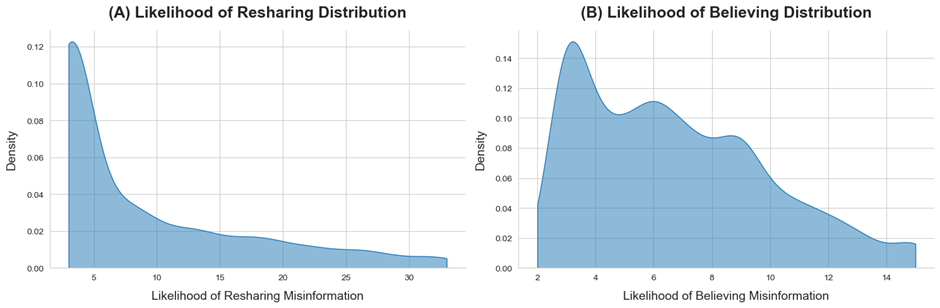
Figure 1. Likelihood of sharing and the likelihood of believing misinformation distributions
Figure 2 shows the Spearman correlation between variables. The correlation matrix reveals that Likelihood of sharing and Likelihood of Believing are correlated with each other with a correlation coefficient of 0.63.
Likelihood of sharing does not share high correlation coefficients with any input features. Among the highest correlation pairs are Likelihood of sharing and country (0.36), Likelihood of sharing and conservatism (0.32), Likelihood of sharing and shared_while_knowing (0.28) and Likelihood of sharing and shared_found_later (0.27). Likelihood of Believing is also not highly correlated with any input variable. The highest correlation pairs are Likelihood of Believing and conservatism (0.35), Likelihood of Believing and country (0.28), and Likelihood of Believing and openness. (-0.26)
No collinearity between the input features is observed in this dataset. The highest correlation pairs include: conservatism and openness (-0.41), shared_while_knowing and shared_found_later (0.36), neuroticism and extraversion (-0.37), agreeableness and conscientiousness (0.49), agreeableness and neuroticism (-0.34).

Figure 2. Spearman correlation matrix between variables
The relationships between likelihood of sharing and a few key variables are shown in Figure 3. For Figures 3A-3D, we plot the percentiles of likelihood of believing, openness, neuroticism, and conservatism against likelihood of sharing to better visualize the relationships. We calculate the percentile ranking of the traits, convert them into percentages, then calculate the mean Likelihood of sharing for each percentile increment. For Figures 3E-3H, the mean likelihood of sharing is plotted against input categorical variables gender, sm_usage, shared_found_later, and shared_while_knowing.
Figure 3B shows that openness and Likelihood of sharing have a generally negative relationship, whereas the relationships between Likelihood of sharing and Likelihood of Believing (Figure 3A) and conservatism (Figure 3D) are positive. The relationship between likelihood of sharing and neuroticism is ambiguous (Figure 3C). Figure 3E also reveals that men are more likely to share than women. Additionally, Figure 3F suggests that those who use social media less often are more likely to share the misinformation. Finally, those who had previously knowingly or unknowingly shared misinformation are shown to be more likely to share misinformation than those who hadn’t (Figure 3G-H).
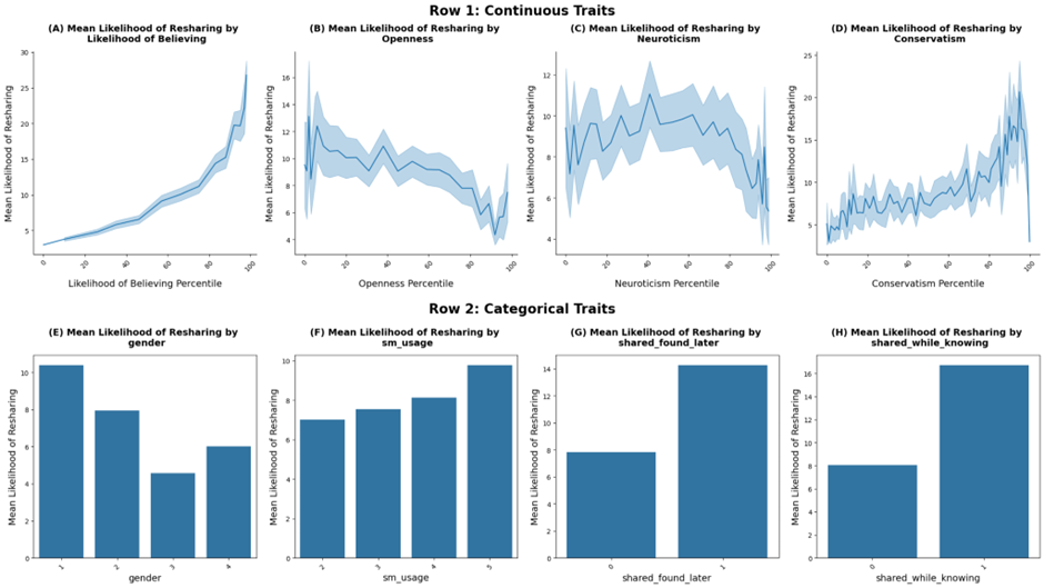
Figure 3. Relationships between likelihood of sharing and key input variables
Figure 4 illustrates the relationships between Likelihood of Believing and other key variables. Likelihood of Believing shares a negative relationship with openness (Figure 4A) and agreeableness (Figure 4B), and has a positive relationship with conservatism (Figure 4C). Additionally, the data suggests that men are slightly more likely to believe right wing misinformation than women (Figure 4D), and that individuals who use social media less frequently are more likely to believe the misinformation (Figure 4E). Furthermore, there is a negative relationship between Likelihood of Believing and age (Figure 4F), with those in the older age group being less likely to believe the right-wing misinformation. Finally, those who had previously unknowingly shared misinformation are found to be more likely to believe the provided misinformation (Figure 4G).

Figure 4. Relationships between likelihood of believing and key input variables
We also plot the relationships between key input variables (Figure 5) to further understand the dataset. We found that openness and conservatism have a negative relationship. Those more right leaning were found to have lower levels of openness (Figure 5A-B). Country and conservatism were also found to have a relationship within this dataset (Figure 5C), where those from the US had a higher mean conservatism rating as opposed to those from the UK. Agreeableness and extraversion were found to have a slightly positive correlation (Figure 5D). Neuroticism and extraversion (Figure 5E) as well as neuroticism and conscientiousness display a negative relationship (Figure 5F)

Figure 5. Relationships between input variables
Methodology
Data Pre-Processing
Due to the data’s self-reported nature, users’ exact numeric responses may be subject to reference bias. Treating this as a classification problem allows for increased interpretability and aligns more with real-world goals of targeting users for intervention. We acknowledge the risk of information loss through dichotomization, but decided on this method for its practical applicability for decision making22.
The next question that arises is: where should the thresholds be drawn? As there is no universal method of selecting thresholds, and thus follow through with multiple approaches as shown in Table 2. For each output variable, we split the data into 2 classes as well as 3 classes. When splitting into 2 classes, we attempt two different thresholds. One threshold is chosen based on the mean value of all responses (mean Likelihood of sharing is 9, mean Likelihood of Believing is 6). This is because it represents the central tendency of data and aligns with common practice in ordinal data analysis23. The other threshold is chosen based on the midpoint value of the range as it provides a neutral reference for classification and ensures an equal-range split24.
When splitting the data into 3 categories, we set thresholds by evenly splitting the range into thirds to maintain equal-width intervals to maintain balance in analysis, an important factor in data analysis as research has shown25. The purpose of introducing a “neutral” class was to understand the factors determining a user’s ambivalence towards a piece of misinformation, as these stakeholders could be crucial targets for online intervention.
| Target Variable | Threshold(s) | Description |
| Likelihood of sharing, likelihood of sharing (range 3-33) | ≤9: unlikely to share >9: likely to share | Threshold is chosen based on mean value of likelihood of sharing |
| ≤15: unlikely to share >15: likely to share | Threshold is chosen based on midpoint of likelihood of sharing range | |
| <13: unlikely to share 13 ≤ and <23: neutral ≥23: likely to share | Two thresholds are chosen to divide the likelihood of sharing scale into three equal parts | |
| Likelihood of believing, Likelihood of Believing (range 3-15) | <6: don’t believe to be true ≥6: believe to be true | Threshold is chosen based on mean value of likelihood of believing |
| <8: don’t believe to be true ≥8: believe to be true | Threshold is chosen based on midpoint of likelihood of believing range | |
| <7: don’t believe to be true 7≤ and <11: neutral ≥11: believe to be true | Two thresholds are chosen to divide the likelihood of believing scale into three equal parts |
Models and Evaluation Metrics
To develop each machine learning model, the data is split into a training set and a testing set. Specifically, 80% of the data is allocated for training and 20% for testing. We also stratify the data to maintain the class distribution in both the training and testing sets.
In this study, we implement two ensemble based machine learning models and one single-model approach. Firstly, we implement Random Forest models, which create a set of decision trees on various subsets of the training data. The votes of the decision trees are then counted to determine the final prediction26. Since the individual models make decisions independently, Random Forest classifiers can avoid overfitting and can model complex nonlinear relationships, thus often have the advantage of high accuracy27.
The second model used is XGBoost, which implements gradient boosting. XGBoost builds decision tree models sequentially, where each new model corrects the error of the previous one28. XGBoost’s advantages lie in its high predictive accuracy as well as its speed. However, it is resource intensive and requires tuning a long list of parameters for optimal performance.
The single-model approach includes logistic regression, which uses a logistic function to predict the probability that an observation belongs to a particular class. It is well-regarded for its simplicity and speed but struggles with non-linear and complex data29. We include logistic regression results to contextualize performance gains and quantify performance improvements. The discussion and analysis will focus on the results of ensemble-based machine learning models because they generally offer more robust performance when handling non-linear and imbalanced data.
To evaluate the performances of the models, we used precision, recall, and F1 scores. Precision measures out of all those predicted positive, how many of them are actually positive. Recall calculates out of all of those actually positive, how many were captured by the model. F1 score seeks to find a balance between precision and recall. Furthermore, model performances are evaluated by comparing train and test results. We aim to balance the model’s precision, recall, and F1 between train and test to avoid overfitting.
In order to compare model performance across thresholds, Receiver Operating Characteristic Area Under Curve scores are calculated for each model, which measures the probability of ranking a random positive instance higher than a random negative instance. With values ranging from 0 to 1, higher AUC values denote a perfect classifier, while a score of 0.5 denotes a random classifier.
All evaluation metrics and AUC scores are presented with bootstrapped confidence intervals at a 95% confidence interval and 1000 samples (a reliable quantity as supported by research30 in order to quantify estimation uncertainty.
Finally, we also conduct McNemar’s test, which is a statistical test assessing whether there is a statistically significant difference between the classification error rates of two models when tested on identical paired predictions. The test is implemented between Random Forest and XGBoost models for all binary classification models to strengthen the rigour of model comparisons.
Hyperparameter tuning
To achieve the best model performance, we tune the models according to their various hyperparameters. Hyperparameters are important properties that define the machine learning process, influencing factors such as model complexity and learning rate. In this process, we use grid search, a method that tries every possible combination of hyperparameters, to find optimal results31. We implement grid search with parameters stratified ‘cross_validation=3’ and weighted F1 scores to address the data imbalance.
For Random Forest, we adjust three key hyperparameters (Table 3): n_estimators, which is the number of decision trees in the forest; min_samples_split, which sets the minimum number of samples required to split an internal node; and max_features, which defines the maximum number of features to consider for the best split. Increasing n_estimators generally enhances accuracy but may lead to longer training times. Modifying max_features influences the diversity of trees, and adjusting min_samples_split can help prevent overfitting28. With 18 input features, we intentionally chose a wide range for max_features (1–17) to ensure we did not overlook potential sweet spots for optimal performance. This range inherently includes common default values such as sqrt(n_features) (~4.24) and log2(n_features) (~4.17), as well as other potential configurations that might better suit our dataset. By exploring this broader range, we aimed to maximize the robustness of our hyperparameter search. For XGBoost, we adjust four key parameters: eta, which controls the learning rate; subsample, which specifies the fraction of samples used for training each tree; colsample_bytree, which determines the fraction of features to consider for each tree; and n_estimators, which is the total number of trees in the model (Table 3). Tuning these parameters can significantly affect model performance. Decreasing eta can lead to more gradual learning, potentially improving accuracy but requiring more trees. Adjusting subsample helps prevent overfitting by introducing randomness, while modifying colsample_bytree influences tree diversity, enhancing the model’s ability to generalize to new data (27). These details of model parameters and their ranges are summarized in Table 3.
| Model | Parameter | Description | Range/Values |
| Random Forest Classifier | n_estimators | number of decision trees | 100, 500 |
| min_samples_split | minimum number of samples required to split an internal node | 20-120, increments of 10 | |
| max_features | maximum number of features to consider when looking for the best split | 1-17 | |
| XGBoost Classifier | eta | step size shrinkage used to prevent overfitting | 0.01, 0.05, 0.1, 0.2, 0.3 |
| subsample | ratio of subsample size to the training data size | 0.5-1.0, increments of 0.1 | |
| colsample_bytree | subsample ratio of columns when constructing each tree | 0.5-1.0, increments of 0.1 | |
| n_estimators | number of trees in the model | 50, 100, 500 |
Handling Class Imbalance
After thresholding Likelihood of sharing and Likelihood of Believing into different classes, we encounter class imbalances. In this section, we explore the different imbalances and discuss methods used to handle the imbalance.
Figure 6 shows the count distribution of the likelihood of sharing for the 3 different classification approaches. In Figures 6A-C, the “unlikely” class is the majority class. In Figure 6A, the “unlikely” class is roughly two times the size of “likely”. For 6B, the “unlikely” class size roughly doubles. In Figure 6C, “unlikely” is the majority class, followed by the “Neutral” class, followed by the “Likely” class.
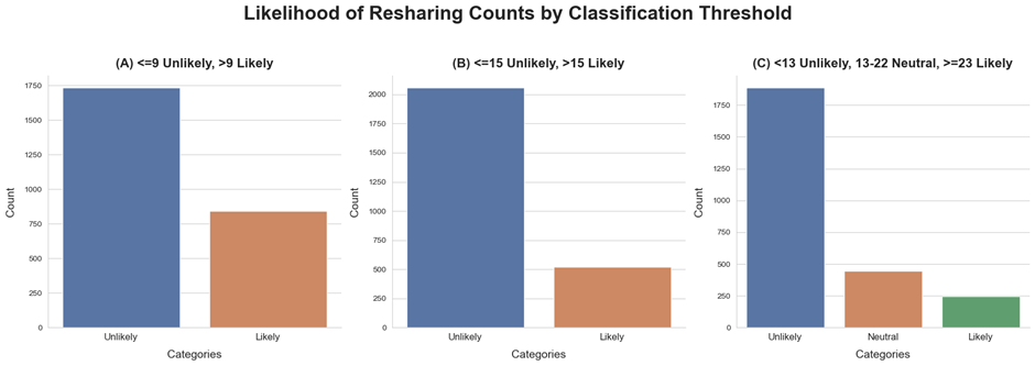
Figure 6. Count distributions of likelihood of sharing categories for a given threshold
Figure 7 shows the count distribution of likelihood of believing for the 3 different classification approaches. In Figure 7A, the “likely” class is the majority class. In 7B, the “unlikely” class is the majority class. In 7C, the “unlikely” class takes majority, and is roughly 1.5 times the size of the “neutral” class, and 4 times the size of the “likely” class.
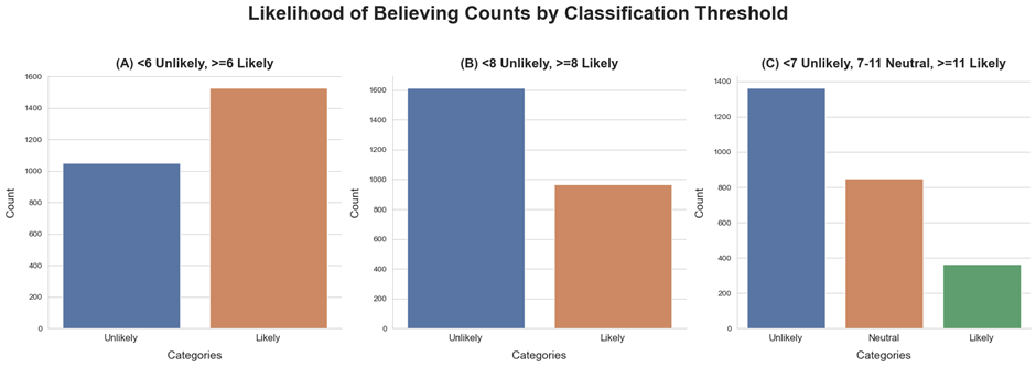
Figure 7. Count distribution of Likelihood of Believing categories
When building the models, we implement different methods to handle class imbalances. The first approach was using the full dataset while applying the code ‘class_weight=balanced’ for Random Forest and ‘scale_pos_weight=number of samples/(2*number of minority class samples)’ for XGBoost. ‘Class_weight’ adjusts weights inversely proportional to class frequencies to improve the model’s attention and thus performance on minority classes28. Scale_pos_weight adjusts the contribution of each class to the loss function during training to avoid bias towards the majority class.
The next approach was undersampling. This sampling technique keeps all the data of the minority class but reduces the size of the majority class. A disadvantage of this approach is its loss of relevant information that could reveal patterns32.
Finally, we attempt a combination of undersampling and oversampling to retain more majority class diversity while still reducing data imbalance33. We first undersample the majority class to 1.5 *size of the minority class, a common ratio used within over- and under-sampling hybrid approaches34. We then oversample the minority class to the same level using the Synthetic Minority Oversampling Technique (SMOTE), a technique that generates synthetic samples through an interpolation of the original data35. Categorical variables (e.g. ‘Country’) inherit categorical values from the nearest minority-class neighbours35. Although SMOTE mitigates bias towards the majority class, it also risks introducing noise, causing the model to overfit to synthetic data. SMOTE can lead to overfitting, particularly when synthetic samples are generated in sparse or noisy regions of feature space. The model may learn patterns that are not generalizable to unseen data. The synthetic samples may not represent realistic or meaningful data points, especially in cases where the minority class has complex distributions or overlaps significantly with the majority class. This can blur decision boundaries36.
Feature Importance Analysis
While one aim of this study was to build a predictive model, we also conduct feature importance analysis to gain insight into how each variable contributes to the model’s predictions, potentially revealing meaningful patterns. Specifically, we will examine the SHAP (SHapley Additive exPlanations) values of the best performing models for the prediction of the output variables. SHAP uses a game-theory approach to assign a numerical value to each feature, illustrating how much that feature influenced the model’s final predictions37. This structured approach enables us to understand feature importance within the model in a clear and interpretable way. By leveraging SHAP, we can better communicate the model’s behavior to stakeholders and use the insights gained to refine our features and improve model performance.
Results
Models Analysis
The two tables below summarize the results from applying three different thresholds using undersampled data. Results regarding original data with class weight balancing and with the undersampling/SMOTE hybrid can be found in the appendix for simplification. All tables include information regarding precision and recall, but the discussion will be focused on F1 scores. We include results for baseline logistic regression models to contextualize performance gains. The tables also display the best parameters, found using grid search, for Random Forest and XGBoost models.
Models for Likelihood of sharing
Table A1 presents the results of predicting sharing likelihood using the original dataset with class weight balancing. The Random Forest model excels with a threshold of 9, achieving an F1 test score of 0.79 ± 0.03 for “unlikely to share” and 0.64 ± 0.06 for “likely to share,” with minimal difference compared to XGBoost, which scores 0.78 ± 0.03 and 0.65 ± 0.05, respectively. Both models show noticeable overfitting for the “likely to share” class, with Random Forest dropping from a training AUC score of 0.93 ± 0.01 to 0.80 ± 0.04, while XGBoost falls from 0.97 ± 0.01 to 0.79 ± 0.04. McNemar’s test comparing the XGBoost and RF models found no significant statistical difference between them (chi-squared=0.82, p-value=0.53). At threshold 15, XGBoost and Random Forest perform similarly for both class predictions. McNemar’s test suggested no significant statistical difference between models (chi-squared=0.039, p-value=0.84). Despite better performance for “unlikely to share” at threshold 15 than at threshold 9, both models perform worse for “likely to share” compared to threshold 9 and demonstrate increased overfitting. Finally, with the two threshold approach, both models struggle with predicting the “neutral” and “likely to share” categories, likely due to data imbalance. Overall, both models exhibit overfitting, with XGBoost demonstrating more severe overfitting.
Table 4 presents the results for predicting likelihood of sharing using undersampled data. All results for threshold 9 and 15 outperform those from the original dataset (Table A1) in predicting the “likely to share” class. The top-performing model is the Random Forest with a threshold of 15, achieving F1 test scores of 0.83 ± 0.03 for “unlikely to share” and 0.80 ± 0.02 for “likely to share.” In comparison, the XGBoost model at threshold 15 scores slightly lower, with F1 scores of 0.76 ± 0.03 and 0.78 ± 0.06 for “unlikely” and “likely to share,” respectively. McNemar’s test comparing the models for both thresholds suggest statistically significant difference (threshold 9: chi-squared=12.99, p-value=0.0003. Threshold 15: chi-squared=24.51, p-value=0.0146). While Random Forest slightly outperforms XGBoost for the two-threshold approach (AUC=0.81 ± 0.04 vs. 0.79 ± 0.04), both models struggle significantly with predicting categories “neutral” and “likely to share,” with F1 scores below 0.50. The uncertainty values for these categories are also significant. For instance, the RF “neutral” category test F1 score is 0.32 ± 0.08, constituting an uncertainty of 25%. The XGBoost models across thresholds struggle with overfitting, reaching training AUC scores of 1.00 ± 0.00 while dropping to test AUC scores of ~0.80.
| Threshold Approach | Model | Train/ Test | Class | Precision | Recall | F1 | AUC | Sample Counts |
| Mean threshold ≤9: unlikely to share >9: likely to share | Logistic Regression (Baseline) | Train | Unlikely to Share | 0.70 ± 0.03 | 0.77 ± 0.03 | 0.73 ± 0.02 | 0.79 ± 0.02 | 675 |
| Likely to Share | 0.74 ± 0.03 | 0.67 ± 0.03 | 0.70 ± 0.03 | 675 | ||||
| Test | Unlikely to Share | 0.80 ± 0.04 | 0.76 ± 0.04 | 0.78 ± 0.04 | 0.77 ± 0.04 | 347 | ||
| Likely to Share | 0.60 ± 0.06 | 0.67 ± 0.07 | 0.63 ± 0.05 | 169 | ||||
| Random Forest {‘max_features’: 4, ‘min_samples_split’: 20, ‘n_estimators’: 500} | Train | Unlikely to share | 0.88 ± 0.03 | 0.89 ± 0.02 | 0.89 ± 0.02 | 0.96 ± 0.01 | 675 | |
| Likely to share | 0.89 ± 0.02 | 0.88 ± 0.02 | 0.88 ± 0.02 | 675 | ||||
| Test | Unlikely to share | 0.83 ± 0.05 | 0.73 ± 0.05 | 0.78 ± 0.04 | 0.79 ± 0.04 | 347 | ||
| Likely to share | 0.60 ± 0.06 | 0.73 ± 0.07 | 0.66 ± 0.05 | 169 | ||||
| XGboost {‘colsample_bytree’: 0.5, ‘eta’: 0.01, ‘n_estimators’: 1000, ‘subsample’: 0.7} | Train | Unlikely to share | 0.99 ± 0.01 | 0.93 ± 0.02 | 0.96 ± 0.01 | 1.00 ± 0.00 | 675 | |
| Likely to share | 0.94 ± 0.02 | 0.99 ± 0.01 | 0.96 ± 0.01 | 675 | ||||
| Test | Unlikely to share | 0.84 ± 0.04 | 0.59 ± 0.05 | 0.69 ± 0.04 | 0.78 ± 0.04 | 347 | ||
| Likely to share | 0.52 ± 0.06 | 0.80 ± 0.06 | 0.63 ± 0.05 | 169 | ||||
| Midpoint threshold ≤15: unlikely to share >15: likely to share | Logistic Regression (Baseline) | Train | Unlikely to Share | 0.75 ± 0.04 | 0.80 ± 0.04 | 0.78 ± 0.03 | 0.86 ± 0.02 | 417 |
| Likely to Share | 0.79 ± 0.04 | 0.74 ± 0.04 | 0.76 ± 0.03 | 417 | ||||
| Test | Unlikely to Share | 0.90 ± 0.03 | 0.78 ± 0.04 | 0.84 ± 0.03 | 0.79 ± 0.05 | 412 | ||
| Likely to Share | 0.47 ± 0.07 | 0.69 ± 0.08 | 0.56 ± 0.07 | 104 | ||||
| Random Forest {max_features: 2, min_samples_split: 70, n_estimators: 500} | Train | Unlikely to share | 0.82 ± 0.04 | 0.82 ± 0.04 | 0.82 ± 0.03 | 0.90 ± 0.02 | 417 | |
| Likely to share | 0.82 ± 0.04 | 0.82 ± 0.03 | 0.82 ± 0.03 | 416 | ||||
| Test | Unlikely to share | 0.90 ± 0.03 | 0.77 ± 0.04 | 0.83 ± 0.03 | 0.80 ± 0.05 | 412 | ||
| Likely to share | 0.83 ± 0.04 | 0.78 ± 0.08 | 0.80 ± 0.02 | 104 | ||||
| XGboost {‘colsample_bytree’: 0.6, ‘eta’: 0.2, ‘n_estimators’: 500, ‘subsample’: 0.7} | Train | Unlikely to share | 1.00 ± 0.00 | 1.00 ± 0.00 | 1.00 ± 0.00 | 1 | 417 | |
| Likely to share | 1.00 ± 0.00 | 1.00 ± 0.00 | 1.00 ± 0.00 | 416 | ||||
| Test | Unlikely to share | 0.90 ± 0.04 | 0.65 ± 0.04 | 0.76 ± 0.03 | 0.76 ± 0.05 | 412 | ||
| Likely to share | 0.76 ± 0.06 | 0.81 ± 0.05 | 0.78 ± 0.06 | 104 | ||||
| Multiple thresholds <13: unlikely to share 13≤ and <23: neutral ≥23: likely to share | Logistic Regression | Train | Unlikely to share | 0.64 ± 0.06 | 0.72 ± 0.06 | 0.68 ± 0.05 | 0.79 ± 0.03 | 198 |
| Neutral | 0.48 ± 0.08 | 0.39 ± 0.07 | 0.43 ± 0.07 | 198 | ||||
| Likely to share | 0.64 ± 0.07 | 0.68 ± 0.07 | 0.66 ± 0.06 | 198 | ||||
| Test | Unlikely to share | 0.89 ± 0.04 | 0.69 ± 0.05 | 0.78 ± 0.03 | 0.78 ± 0.04 | 377 | ||
| Neutral | 0.27 ± 0.08 | 0.36 ± 0.10 | 0.31 ± 0.08 | 89 | ||||
| Likely to share | 0.32 ± 0.09 | 0.68 ± 0.13 | 0.43 ± 0.10 | 50 | ||||
| Random Forest {max_features: 1, min_samples_split: 30, n_estimators: 500} | Train | Unlikely to share | 0.78 ± 0.05 | 0.86 ± 0.05 | 0.81 ± 0.04 | 0.93 ± 0.01 | 199 | |
| Neutral | 0.81 ± 0.06 | 0.68 ± 0.07 | 0.74 ± 0.05 | 198 | ||||
| Likely to share | 0.80 ± 0.05 | 0.85 ± 0.05 | 0.83 ± 0.04 | 198 | ||||
| Test | Unlikely to share | 0.88 ± 0.04 | 0.72 ± 0.04 | 0.79 ± 0.03 | 0.81 ± 0.04 | 377 | ||
| Neutral | 0.29 ± 0.09 | 0.35 ± 0.10 | 0.32 ± 0.08 | 89 | ||||
| Likely to share | 0.36 ± 0.10 | 0.74 ± 0.12 | 0.48 ± 0.10 | 50 | ||||
| XGboost {‘colsample_bytree’: 0.5, ‘eta’: 0.01, ‘n_estimators’: 500, ‘subsample’: 0.8} | Train | Unlikely to share | 0.98 ± 0.02 | 1.00 ± 0.00 | 0.99 ± 0.01 | 1.00 ± 0.00 | 199 | |
| Neutral | 1.00 ± 0.00 | 0.98 ± 0.02 | 0.99 ± 0.01 | 198 | ||||
| Likely to share | 0.99 ± 0.01 | 0.99 ± 0.01 | 0.99 ± 0.01 | 198 | ||||
| Test | Unlikely to share | 0.90 ± 0.03 | 0.67 ± 0.05 | 0.77 ± 0.04 | 0.79 ± 0.04 | 377 | ||
| Neutral | 0.31 ± 0.08 | 0.47 ± 0.10 | 0.37 ± 0.08 | 89 | ||||
| Likely to share | 0.35 ± 0.10 | 0.68 ± 0.14 | 0.46 ± 0.10 | 50 |
Table A2 displays the results after implementing a combination of undersampling and oversampling data balancing techniques. At threshold 9, Random Forest achieves an F1 test score of 0.78 ± 0.04 for “unlikely to share” and 0.63 ± 0.06 for “likely to share,” with results similar to XGBoost, which scores 0.76 ± 0.04 and 0.64 ± 0.06, respectively. McNemar’s test comparing the models found no significant statistical difference (chi-squared=0.37, p-value=0.54). At threshold 15, the models excel at predicting “unlikely to share,” boasting scores of 0.84 ± 0.03 and 0.81 ± 0.03 for Random Forest and XGBoost respectively. Both models struggle with predicting “likely to share,” achieving F1 scores slightly above 0.50. McNemar’s test found no significant statistical difference (chi-squared=0.019, p-value=0.892). With two thresholds, both models struggle. While excelling at predicting the “unlikely” category (Random Forest scores 0.80 ± 0.03, XGBoost scores 0.76 ± 0.04) both models struggle with predicting the “likely” and “neutral” categories (“neutral”: RF scores 0.37 ± 0.08 and XGBoost scores 0.39 ± 0.07). Both models show noticeable overfitting across thresholds, with XGBoost more prone (dropping from AUC train score of 1.00 ± 0.00 to ~0.80 test scores)
The ROC curves for the Random Forest and XGBoost classifiers for the highest performing models for predicting sharing (undersampled data, threshold 15) are presented in Figure 8. Both models demonstrated comparable discriminative performance, with Random Forest achieving an area under the curve (AUC) of 0.80 (95% CI: 0.75-0.85) and XGBoost achieving an AUC of 0.76 (95% CI: 0.71-0.81) – a non-significant difference as demonstrated by overlapping confidence intervals. However, the precision-recall curves demonstrate more pronounced differences, particularly in the high-precision/low recall regions, where Random Forest maintained higher performance, a result which can be supported by the McNemar test (p-value=0.015).
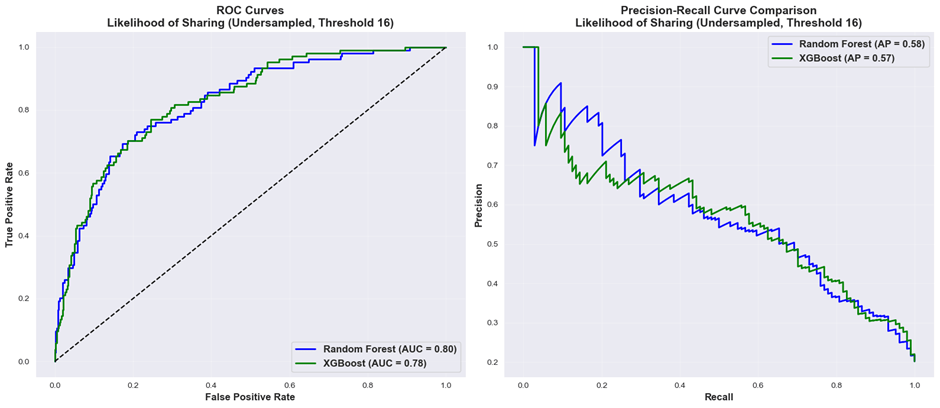
Figure 8. ROC Curves and Precision-Recall Curves for Random Forest and XGBoost (“Likelihood of Sharing”, undersampled data, threshold 16)
Models for Likelihood of Believing
Table A3 presents the results of predicting believing likelihood using the original dataset with class weight balancing. The Random Forest model excels with a threshold of 6, achieving an F1 test score of 0.61 ± 0.06 for “unlikely to believe” and 0.73 ± 0.04 for “likely to believe,” slightly outperforming XGBoost, which scores 0.62 ± 0.05 and 0.72 ± 0.04, respectively. At threshold 8, Random Forest marginally outperforms XGBoost for both classes. Both models struggle to predict “likely to believe” (0.55 ± 0.06 for Random Forest, 0.54 ± 0.06 for XGBoost). Despite better performance predicting for “unlikely to believe” at threshold 8 compared to threshold 6, both models perform worse in predicting “likely to believe.” With two thresholds, both models struggle with the “neutral” and “likely to believe” categories, likely due to data imbalance. Random Forest scores 0.69 ± 0.04 for “unlikely to believe,” while XGBoost scores 0.73 ± 0.04, but Random Forest outperforms XGBoost in the “likely to believe” categories (0.41 ± 0.09 vs. 0.35 ± 0.12). F1 scores for the “neutral” class are 0.40 ± 0.07 and 0.41 ± 0.07 for RF and XGboost respectively. Both models show noticeable overfitting across all thresholds. For instance, for threshold 6, Random Forest drops from a training AUC score of 0.97 ± 0.01 to 0.74 ± 0.04, and XGBoost’s AUC scores drop from 0.95 ± 0.01 to 0.74 ± 0.04 between train and test. McNemar’s tests for both thresholds found no statistically significant difference between the models (threshold 6: chi-squared=0.2, p-value=0.65, threshold 8: chi-squared=1.29, p-value=0.26).
Table 5 presents the results of predicting Likelihood of Believing using the undersampled dataset. The best performing model below is the Random Forest model with a threshold of 6, achieving an F1 test score of 0.61 ± 0.05 for “unlikely to share” and 0.67 ± 0.04 for “likely to share,” slightly outperforming XGBoost, which scores 0.63 ± 0.05 and 0.64 ± 0.05, respectively. Both models exhibit significant overfitting, as indicated by training AUC scores exceeding 0.9 for both classes, which decline by more than 0.2 on the test data. McNemar’s test suggested no significant difference between the models (chi-squared=0.46, p-value=0.5) At threshold 8, Random Forest outperforms XGBoost for “unlikely to believe” (0.69 ± 0.04 vs. 0.59 ± 0.05) and perform the same for “likely to believe” (a mean of 0.57). Compared to threshold 6, Random Forest shows slightly lower results for “unlikely”, while results slightly improved for “likely,” while XGBoost performs worse for both classes. McNemar’s test found a significant difference between Random Forest and XGBoost predictions (chi-squared=12.01, p-value=0.03). With two thresholds, both models struggle with the “likely to believe” and “neutral” categories. Both models share similar F1 scores for all three categories with overlapping confidence intervals. Random Forest achieves 0.67 ± 0.04, 0.46 ± 0.07, 0.43 ± 0.09 for “unlikely,” “neutral,” and “likely” categories, respectively, while XGBoost achieves 0.65 ± 0.05, 0.44 ± 0.07, 0.40 ± 0.08 for the three categories, respectively. Compared to multiple thresholds from Table A3 (original data), though the performance on predicting “neutral” and “likely to believe” increased, the F1 score for predicting “unlikely to believe” decreased.
| Threshold Approach | Model | Train/ Test | Class | Precision | Recall | F1 | AUC | Sample Counts |
| Mean threshold <6: unlikely to believe ≥6: likely to believe | Logistic Regression (Baseline) | Train | Unlikely to Believe | 0.65 ± 0.03 | 0.66 ± 0.03 | 0.65 ± 0.03 | 0.72 ± 0.02 | 842 |
| Likely to Believe | 0.65 ± 0.03 | 0.64 ± 0.03 | 0.65 ± 0.03 | 841 | ||||
| Test | Unlikely to Believe | 0.56 ± 0.06 | 0.71 ± 0.06 | 0.63 ± 0.05 | 0.74 ± 0.04 | 210 | ||
| Likely to Believe | 0.76 ± 0.06 | 0.61 ± 0.05 | 0.68 ± 0.05 | 211 | ||||
| Random Forest {max_features: 4, min_samples_split: 20, n_estimators: 1000} | Train | Unlikely to believe | 0.91 ± 0.02 | 0.91 ± 0.02 | 0.91 ± 0.01 | 0.97 ± 0.01 | 842 | |
| Likely to believe | 0.91 ± 0.02 | 0.91 ± 0.02 | 0.91 ± 0.01 | 841 | ||||
| Test | Unlikely to believe | 0.55 ± 0.06 | 0.69 ± 0.06 | 0.61 ± 0.05 | 0.73 ± 0.04 | 210 | ||
| Likely to believe | 0.75 ± 0.05 | 0.61 ± 0.06 | 0.67 ± 0.04 | 211 | ||||
| XGboost {‘colsample_bytree’: 0.9, ‘eta’: 0.01, ‘n_estimators’: 1000, ‘subsample’: 0.5} | Train | Unlikely to believe | 0.91 ± 0.02 | 0.99 ± 0.01 | 0.95 ± 0.01 | 0.99 ± 0.00 | 842 | |
| Likely to believe | 0.99 ± 0.01 | 0.90 ± 0.02 | 0.94 ± 0.01 | 841 | ||||
| Test | Unlikely to believe | 0.54 ± 0.05 | 0.77 ± 0.06 | 0.63 ± 0.05 | 0.72 ± 0.05 | 210 | ||
| Likely to believe | 0.78 ± 0.05 | 0.54 ± 0.05 | 0.64 ± 0.05 | 211 | ||||
| Midpoint threshold <8: unlikely to believe ≥8: likely to believe | Logistic Regression (Baseline) | Train | Unlikely to Believe | 0.68 ± 0.03 | 0.72 ± 0.03 | 0.70 ± 0.03 | 0.76 ± 0.02 | 772 |
| Likely to Believe | 0.70 ± 0.03 | 0.66 ± 0.03 | 0.68 ± 0.03 | 772 | ||||
| Test | Unlikely to Believe | 0.72 ± 0.05 | 0.63 ± 0.05 | 0.67 ± 0.04 | 0.70 ± 0.05 | 323 | ||
| Likely to Believe | 0.49 ± 0.06 | 0.59 ± 0.07 | 0.53 ± 0.05 | 193 | ||||
| Random Forest {max_features: 2, min_samples_split: 30, n_estimators: 500} | Train | Unlikely to believe | 0.84 ± 0.03 | 0.84 ± 0.03 | 0.84 ± 0.02 | 0.91 ± 0.01 | 772 | |
| Likely to believe | 0.84 ± 0.03 | 0.84 ± 0.03 | 0.84 ± 0.02 | 772 | ||||
| Test | Unlikely to believe | 0.75 ± 0.05 | 0.64 ± 0.05 | 0.69 ± 0.04 | 0.70 ± 0.05 | 193 | ||
| Likely to believe | 0.52 ± 0.06 | 0.64 ± 0.07 | 0.57 ± 0.06 | 193 | ||||
| XGboost {colsample_bytree: 0.6, eta: 0.01, n_estimators: 500, subsample: 0.5} | Train | Unlikely to believe | 0.96 ± 0.01 | 0.74 ± 0.03 | 0.83 ± 0.02 | 0.96 ± 0.01 | 772 | |
| Likely to believe | 0.79 ± 0.02 | 0.97 ± 0.01 | 0.87 ± 0.02 | 772 | ||||
| Test | Unlikely to believe | 0.75 ± 0.06 | 0.49 ± 0.06 | 0.59 ± 0.05 | 0.70 ± 0.05 | 193 | ||
| Likely to believe | 0.46 ± 0.06 | 0.74 ± 0.06 | 0.57 ± 0.05 | 193 | ||||
| Multiple thresholds <7: unlikely to believe 7≤ and <11: neutral ≥11: likely to believe | Logistic Regression | Train | Unlikely to share | 0.54 ± 0.05 | 0.58 ± 0.06 | 0.56 ± 0.05 | 0.74 ± 0.02 | 293 |
| Neutral | 0.45 ± 0.06 | 0.40 ± 0.06 | 0.42 ± 0.06 | 293 | ||||
| Likely to share | 0.62 ± 0.06 | 0.63 ± 0.06 | 0.62 ± 0.05 | 293 | ||||
| Test | Unlikely to share | 0.71 ± 0.06 | 0.60 ± 0.06 | 0.65 ± 0.05 | 0.73 ± 0.03 | 273 | ||
| Neutral | 0.46 ± 0.08 | 0.39 ± 0.07 | 0.42 ± 0.07 | 170 | ||||
| Likely to share | 0.33 ± 0.08 | 0.64 ± 0.11 | 0.44 ± 0.09 | 73 | ||||
| Random Forest {‘max_features’: 10, ‘min_samples_split’: 20, ‘n_estimators’: 500} | Train | Unlikely to believe | 0.86 ± 0.04 | 0.89 ± 0.04 | 0.87 ± 0.03 | 0.97 ± 0.01 | 293 | |
| Neutral | 0.91 ± 0.03 | 0.84 ± 0.04 | 0.88 ± 0.03 | 292 | ||||
| Likely to believe | 0.85 ± 0.04 | 0.89 ± 0.04 | 0.87 ± 0.03 | 293 | ||||
| Test | Unlikely to believe | 0.75 ± 0.06 | 0.61 ± 0.06 | 0.67 ± 0.04 | 0.73 ± 0.04 | 273 | ||
| Neutral | 0.48 ± 0.08 | 0.44 ± 0.08 | 0.46 ± 0.07 | 170 | ||||
| Likely to believe | 0.33 ± 0.08 | 0.62 ± 0.11 | 0.43 ± 0.09 | 73 | ||||
| XGboost {‘colsample_bytree’: 0.5, ‘learning_rate’: 0.01, ‘n_estimators’: 1000, ‘subsample’: 0.7, ‘random_state’: 1} | Train | Unlikely to believe | 1.00 ± 0.00 | 1.00 ± 0.00 | 1.00 ± 0.00 | 1.00 ± 0.00 | 293 | |
| Neutral | 1.00 ± 0.00 | 1.00 ± 0.00 | 1.00 ± 0.00 | 292 | ||||
| Likely to believe | 1.00 ± 0.00 | 1.00 ± 0.00 | 1.00 ± 0.00 | 293 | ||||
| Test | Unlikely to believe | 0.75 ± 0.06 | 0.58 ± 0.06 | 0.65 ± 0.05 | 0.71 ± 0.04 | 73 | ||
| Neutral | 0.44 ± 0.07 | 0.44 ± 0.07 | 0.44 ± 0.07 | 74 | ||||
| Likely to believe | 0.31 ± 0.08 | 0.56 ± 0.11 | 0.40 ± 0.08 | 73 |
Table A4 summarizes the results of predicting Likelihood of Believing using a combination of undersampling and oversampling. At a threshold of 6, the Random Forest model performs slightly better in predicting both classes, achieving scores of 0.60 ± 0.06 for “unlikely to believe” and 0.72 ± 0.04 for “likely to believe,” compared to 0.58 ± 0.05 and 0.69 ± 0.04, respectively, for XGBoost. McNemar’s test found no significant difference between the two models (chi-squared=2.05, p-value=0.15) At a threshold of 8, the Random Forest model outperforms XGBoost for the “unlikely” class, scoring 0.73 ± 0.04 as opposed to 0.70 ± 0.04, whereas it scores lower for the “likely” class (0.54 ± 0.06 vs. 0.58 ± 0.05). Compared to the threshold of 6, both models show improvement in predicting “unlikely to believe” by approximately 0.10, but their performance in predicting “likely to believe” declines by about 0.10. McNemar’s test found no significant difference between the two models (chi-squared=0.42, p-value=0.52). For both thresholds, both models struggle with the “neutral” class, each scoring below 0.5. Random Forest slightly outperforms XGBoost in predicting “unlikely to believe” (0.62 ± 0.05 vs. 0.61 ± 0.05 as well as in predicting “likely to believe” (0.42 ± 0.09 vs. 0.37 ± 0.10). All Random Forest and XGBoost models in Table A4 exhibit significant overfitting, with training AUC scores ranging from 0.97 to 1.00, which drop by more than 0.20 in testing.
The ROC and precision-recall curves for the Random Forest and XGBoost classifiers for predicting belief (original data with class weight balancing, threshold 6) are presented in Figure 9. Both models demonstrated comparable discriminative performance, with Random Forest achieving an area under the curve (AUC) of 0.73 (95% CI: 0.69-0.77) and XGBoost achieving an AUC of 0.72 (95% CI: 0.68-0.76). The curves largely overlapped across all thresholds, indicating similar ability to distinguish between positive and negative cases. Given the negligible difference in AUC values, as well as McNemar’s test results (p-value=0.65), both approaches appear equally effective for this prediction task.
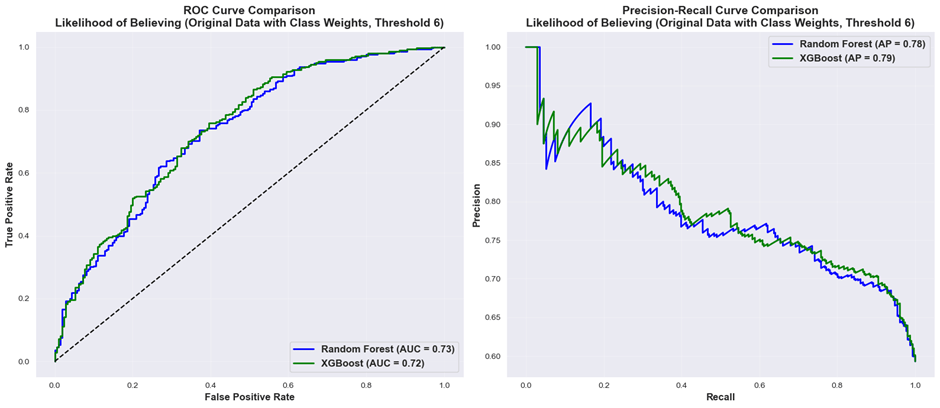
Figure 9. ROC Curves and Precision-Recall Curves for Random Forest and XGBoost (Likelihood of Believing, original data with class weight balancing, threshold 6)
Feature Importance Analysis
In this section, the SHAP results of the top models for predicting “likelihood of sharing” and “likelihood of believing” will be discussed. For “likelihood of sharing”, we will examine SHAP values of the Random Forest using threshold 15 and undersampled data (Table 5). For “likelihood of believing”, we examine the SHAP values of the Random Forest model using the threshold 6 and original dataset (Table A3). Specifically, results below display predictions for the positive class, “likely to share/believe”.
Figure 10 displays the mean SHAP value of every input variable for predicting “likely to share.” Figure 10A illustrates that the highest contributing variables to the model’s predictions are country, conservatism, shared_found_later and gender, while the least impactful variables are consensus, authoritative, and age_group.
Figure 10B illustrates the relationship between input feature value and the impact on the model’s prediction. Figure 10B suggests a country value of “UK” is associated with a higher likelihood of sharing misinformation than respondents. Figure 10B also reveals that high levels of conservatism and having previously knowingly or unknowingly shared misinformation are associated with a higher prediction of sharing. Additionally, a female gender is associated with a low prediction of sharing. Of the 5 factor personality traits, openness has the highest impact on the model’s prediction, with lower openness correlating with a higher prediction of sharing. This could be due to confounding between openness and conservatism, as explained by the negative relationship found in data-preprocessing (Figure 5A). Higher levels of extraversion and conscientiousness are linked with higher model predictions, while higher levels of neuroticism and agreeableness correlate with lower predictions. More frequent social media use is associated with a positive model prediction. Though the magnitude of impact is marginal, lower levels of education, greater age, and higher levels of consensus and authoritativeness are associated with positive model output.

Figure 10. SHAP Analysis on best performing model for the prediction of “likely to share”
Figure 11A shows the mean SHAP values for each input variable influencing the prediction of “likely to believe” using our top-performing model. This figure highlights that conservatism, openness, and country are the most significant factors affecting the model’s prediction of belief, whereas consensus, authoritative, and gender have the lowest influence on the model’s predictions.
Figure 11B illustrates the relationship between input feature values and their influence on the model’s prediction of “likelihood of believing.” Consistent with findings related to “likelihood of sharing,” we observe that higher levels of conservatism are linked to an increased model prediction of belief. Variables such as shared_found_later and shared_while_knowing show similar effects as those found in Figure 10B, indicating that having previously shared content, whether knowingly or unknowingly, is associated with higher likelihood of belief. Country of origin plays a significant role; originating from the UK is correlated with a lower likelihood of belief than originating from the US. Additionally, lower levels of education correlate with a higher likelihood of belief and, interestingly, younger age is linked with increased susceptibility to misinformation. In contrast to the “likelihood of sharing,” gender appears to have a minimal impact on the model’s predictions. While higher levels of extraversion and lower levels of agreeableness may somewhat correlate with a greater likelihood of belief, the relationship is not distinctly clear. The effects of neuroticism, occupation, social media usage, conscientiousness, and consensus remain ambiguous.
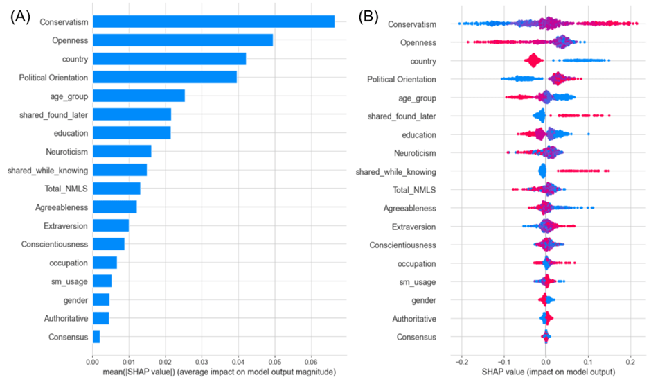
Figure 11. SHAP Analysis on best performing model for the prediction of “likely to believe”
Discussion
In this study, we trained and tested Random Forest and XGBoost models to predict 2 output variables: the likelihood of an individual sharing and believing right-wing misinformation. Through a systematic study examining the effect of different classification thresholds and sampling methods, we were able to build a high performing model to predict an individual’s likelihood of sharing misinformation, and a moderately successful model at predicting an individual’s likelihood of belief based on individual demographic features. In addition, we conducted feature weight analysis on the top performing models and found that country, conservatism, and shared_found_later (whether the individual had previously unknowingly shared misinformation) were the highest determinants of sharing, and conservatism, openness, and country were the highest determinants of belief.
Model Analysis
Figures 12-13 summarize the results of predicting “likelihood of sharing across Random Forest and XGBoost models. Figures 14-15 summarize the results of predicting likelihood of believing across Random Forest and XGBoost models. The F1 scores are the mean of all samples with bootstrapped confidence intervals (1000 samples, 95% CI), with full intervals documented in Tables 4-5 and Appendix.
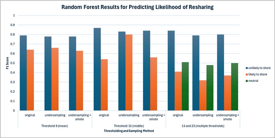
Figure 12. Summary of Random Forest results for predicting likelihood of sharing across thresholding and sampling techniques

Figure 13. Summary of XGBoost results for predicting likelihood of sharing across thresholding and sampling techniques
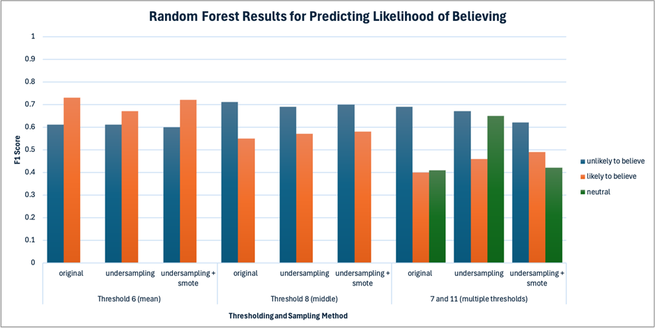
Figure 14. Summary of Random Forest results for predicting likelihood of believing across thresholding and sampling techniques
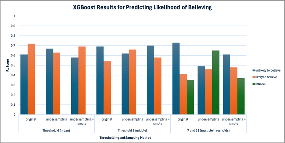
Figure 15. Summary of XGBoost results for predicting likelihood of believing across thresholding and sampling techniques upon existing machine learning-based literature on this subject, shifting focus from content level detection (eg. NLP classification38,39 to user-level susceptibility. While natural language processing approaches can help to identify potentially harmful individual posts, our approach can identify vulnerable users and inform preventative measures unique to our approach. Social media platforms could integrate these models to flag and prioritize review of posts shared by users identified as high-risk for misinformation sharing. Platforms should consider implementing targeted educational prompts and nudges at identified high-risk users before they share posts40. Our work complements existing tools from a crucial behavioural lens.
It is important to recognize that these models were built on a specific, context-based dataset, only reflecting trends among the responses of individuals from the US and UK from 2019 to 2020. Additionally, the models also don’t take into consideration the content or language of the misinformation posts themselves. To improve the results, future works should attempt to build models that center around both post’s content and the viewer’s demographic features, as well as use a larger dataset.
Feature Importance Analysis
Our feature weight analysis reveals that conservatism is a high indicator for sharing (ranked 2nd) and belief (ranked 1st), where greater amounts of conservatism align with greater likelihood of sharing and/or believing the right-wing misinformation as shown in Figures 8B and 9B. This correlation was observed during exploratory data analysis (Figure 3D, Figure 4C), and agrees with existing literature on this subject that suggest that confirmation bias41 and directionally motivated reasoning42 cause individuals to be more inclined to believe and share misinformation aligning with their prior beliefs. It is worth noting that our study only explores interactions with right-wing misinformation.
Country was also found to be a strong predictor of sharing (ranked 1st) and belief (ranked 3rd). Our findings suggest that within the given dataset, representing user reactions to 3 posts on xenophobia and immigration issues from 2019-2020, users from the US were more likely to share and believe the misinformation than users from the UK. Our findings could thus reflect the underlying political and cultural differences between the two countries. Research43,44 found that the US was, on average, more politically polarized than the UK, due to the US having more fragmented media landscape, while the UK had a stronger centralized public broadcasters (eg. BBC). Studies show that political polarization is a key driver of the dissemination of misinformation45,46 as it affects the extent to which users trust media sources. To further explore how country affects users’ interactions with misinformation, future studies are recommended to explore whether the trend observed holds up across different time periods outside of the period of 2019-2020. Researchers should also strive to understand how different topics of misinformation, outside of purely immigration, are perceived by users in different countries, and include a larger variety of countries. This could allow for greater insight to expand on our findings.
While gender was ranked as 4th most impactful variable for sharing (Figure 10A), its impact on belief was negligible (Figure 11A). Figure 10B implies that being male is a large positive indicator for sharing misinformation, whereas being female is a negative indicator on likelihood of sharing. This is a particularly interesting dichotomy, as it suggests that while both genders have similar likelihood of believing misinformation, men are more likely to further disseminate it. Our discovery is consistent from prior findings with men more likely to share misinformation47,48,49. A suggested reason for this is men’s overconfidence in their knowledge and decision-making abilities, causing an increased susceptibility to share misinformation than women50. Men also exhibit more risk-taking behaviours than women, with men being socially expected to be more assertive and opinionated than women51. Our findings indicate that sharing can be driven by factors independent of belief, such as social pressure, or differences in individuals’ cognitive processing, as explained by Social Role Theory52. This reveals a crucial nuance in research regarding misinformation dissemination, encouraging future intervention methods and research to consider how sharing is not always a direct result of belief. Stakeholders could choose to diversify the target audience of nudges or media literacy education to deal with this discrepancy.
The variables shared_found_later and shared_while_knowing were significant predictors of an individual’s likelihood of sharing, ranked 3rd and 5th highest SHAP values respectively. Figure 10B shows that those who had previously unknowingly or knowingly shared misinformation were more likely to share and believe the misinformation, and vice versa. This is highly intuitive, as individuals who have previously shown susceptibility to misinformation or an interest in spreading misinformation are likely to demonstrate similar behaviours, a finding supported by research53 and social learning theory54. This finding suggests that misinformation interventions and anti-misinformation campaigns should be targeted at individuals who have shown previous engagement with misinformation. Platforms should consider targeted warnings and nudges, as well as sharing restrictions for users who show repeated misinformation dissemination behaviour55. Interestingly, shared_found_later and shared_while_knowing were relatively unimpactful in determining belief of the misinformation, which suggests that individuals’ belief of misinformation is not highly related to previous sharing of misinformation.
Openness was a high indicator of belief (ranked 2nd), and had a moderate impact on sharing (ranked 6th). A decrease in openness led to an increase in sharing/belief, a correlation observed in exploratory data analysis (Figure 3 and 4). A correlation between openness and conservatism was also found (Figure 5A and 5B), where more conservative individuals demonstrated lower openness. Considering that an increase in conservatism led to a direct increase in sharing and belief, the role of openness could be attributed to confounding of openness and conservatism. Another possible explanation is that more open individuals tend to engage in more analytical, reflective cognitive behaviours, which can reduce susceptibility to misinformation56,57. While both factors likely play a role, we cannot determine whether and to what extent openness’s role is due to its relationship with ideology or due to inherent cognitive behaviours. It’s important to note that our study only examines the relationship between openness and the sharing of right-wing misinformation, and cannot indicate the role of openness when individuals face left-wing misinformation. It is possible that individuals with higher openness are indeed more likely to share misinformation in line with their ideologies (liberal ideologies).
The role of the New Media Literacy Score (Total_NMLS) is ambiguous. This may be counterintuitive, as many have argued that increase in media literacy causes more critical thinking and reduces the likelihood of disseminating misinformation58,59. Comparatively, our study suggests that personality or social circumstances can outweigh the role of media literacy, or could also indicate that the New Media Literacy Scale doesn’t capture the nuanced nature of media engagement. This is consistent with findings of certain studies60 suggesting that partisanship can override the role of media literacy. While this could be possible explanations for our results, the variable’s insignificance could also be due to the survey data being self-reported in a test setting, which could have affected the validity of an individual’s response.
While age had an impact on belief (ranked 5th most influential variable), it was among the least significant variables for predicting sharing. Interestingly, the model found that the younger an individual, the more likely they were to believe the misinformation. It is important to note that the data used was skewed, with far more young respondents than older ones. However, younger respondents also had larger proportions of left-wing views as opposed to older respondents, which should indicate an opposite trend as the one found (Figure 16). Thus, this prediction is not a reflection of pure data bias.
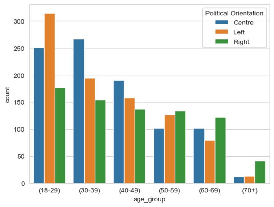
Figure 16. Distribution of input variables age_group by political orientation
Our findings regarding age oppose general consensus, as older generations are associated with higher levels of conservatism and lower media literacy, which should cause higher chances of believing and sharing right-wing misinformation61. In contrast, we suggest that younger social media users are more susceptible to believing a piece of misinformation is true. This could be because young people spend greater amounts of time on social media, leading to more trust in social media headlines62. Dual-process theory suggests that young people may be more reliant on System 1 (automatic and emotional) thinking due to frequent exposure to online content, whereas older generations may rely more on System 2 (analytical) thinking, scrutinizing online content more thoroughly prior to acceptance63. Indeed, our findings are consistent with those found by a 2023 Psychology test by the University of Cambridge64, which surveyed over 8,000 participants over two years. They found that older generations were better able to identify fake news headlines compared to younger generations. They also found that the longer an individual would spend online, the more susceptible they were to believing misinformation. This suggests the need for more targeted media literacy interventions towards young audiences.
Finally, in alignment with Buchanan (2020)16’s study, the post’s authoritativeness and level of consensus was found to have virtually no impact on the model’s prediction. This is contrary to literature suggesting that online content with more authoritative tone and more likes have a higher likelihood of being shared and believed65. Our results could possibly be due to flaws in the survey’s design, where the indicators were possibly not noticeable enough to become impactful. Future studies would benefit from exploring authoritativeness and consensus at a variety of data points, for instance by investigating how a range of different numbers of likes affects a user’s belief and sharing.
Recognizing that this study’s data reflects interactions with right-wing misinformation, future work on this topic could introduce “post’s political orientation” as an additional variable, and include both left and right wing misinformation. This would allow us to further generalize the indicators of sharing and belief, ascertaining the results of this study. This dataset would further benefit from having more balanced responses and similar representation of each category, such as country and age.
While this study’s findings provide robust insights into misinformation sharing and belief in the US and UK in 2019-2020, its generalizability to other temporal and political contexts requires consideration. The US/UK scope of the experiment reflects aspects of Western political discourse, but not non-Western contexts, where political views and issues vary drastically. The survey data was also collected in the pre-pandemic era, whereas post-pandemic era political and economic discourse has shifted since. Findings in this experiment can only apply to misinformation solely composed of text and images. This experiment’s design does not account for the rise of audio-visual based online content as well as AI deep-fakes. These limitations serve as benchmarks for areas of future study.
While prior machine learning-based studies on misinformation focused on content features66,67, we investigate the individual demographic and personality features contributing to misinformation spread. Previous studies investigating a similar topic only employ non-ML based approaches, making our methodological contribution unique. While some studies have investigated demographic features affecting misinformation sharing and belief68,69, this study’s SHAP analysis quantifies the effect of various features and identifies non-linear relationships. These factors make this study’s findings unique.
Furthermore, we conduct a systematic study of multiple thresholds and sampling techniques revealing how a lower classification threshold, as well as undersampling, increases the model’s predictive accuracy. This provides an empirical framework for future machine learning works that use Likert scale data with unbalanced misinformation datasets.
Conclusion
This study uses a unique machine learning approach to understand the extent to which AI models can predict an individual’s sharing and belief of right wing misinformation, and quantifies the contribution of demographic features to the model’s prediction. We use Random Forest and XGBoost models to perform classification, attempting various thresholds and sampling techniques. We build a powerful model with 0.83 ± 0.03 and 0.80 ± 0.02 F1 scores for predicting “unlikely to share” and “likely to share” categories, respectively. The strongest model for predicting belief has F1 scores 0.61 ± 0.06 and 0.73 ± 0.04 for “unlikely to believe” and “likely to believe”, respectively.
Conservatism, country, and an individual’s prior experience sharing misinformation were among the highest determinants of both sharing and belief. Being right-leaning, from the US (as opposed to the UK), and having previously knowingly or unknowingly shared misinformation, caused the models to predict greater likelihood of sharing and believing. Exploring the likelihood of sharing and believing independent of each other, we find that men are more likely to share than women, but their likelihood of believing misinformation is relatively the same. We find that younger individuals are more likely to believe the misinformation, but age doesn’t affect sharing behaviour. Openness was a higher determinant of belief compared to sharing behaviour, where we found that more open individuals were less likely to believe and/or share the misinformation. The media literacy of respondents, as well as authoritativeness and level of consensus displayed on the post, had minimal effect on the model’s predictions.
The machine learning models were built upon imbalanced data that only reflects interactions with right-wing misinformation in 2019-2020. Future studies should aim to collect more balanced data, and could introduce “post’s political orientation” as another input variable. To improve the predictive power of the models, researchers could attempt to combine the exploration of demographic features with textual features as well. These would allow our findings to be more generalizable to a greater variety of misinformation posts, allowing governments and social media companies to take the necessary steps to reduce the dissemination of misinformation.
Ethics
All data used in this experiment was anonymized and taken with consent of the subjects.
The AI prediction of susceptibility to misinformation can raise ethical concerns. There is risk of potential misuse of the predictive modelling approach to profile individuals and a potential breach of privacy. We emphasize critical ethical safeguards of using anonymized and aggregated demographic data to avoid re-identification, and strict prohibitions against profiling individuals if this model is ever deployed. Future applications are urged to consider privacy risks by implementing opt-in consent protocols and the right to data erasure.
Appendix
Table A1. Summary of evaluation metrics for likelihood of sharing using original dataset with class weight balancing
| Threshold Approach | Model | Train/ Test | Class | Precision | Recall | F1 | AUC | Sample counts |
| Mean threshold ≤9: unlikely to share >9: likely to share | Logistic Regression | Train | Unlikely to Share | 0.76 ± 0.02 | 0.88 ± 0.02 | 0.82 ± 0.01 | 0.80 ± 0.02 | 1388 |
| Likely to Share | 0.70 ± 0.04 | 0.51 ± 0.04 | 0.59 ± 0.03 | 675 | ||||
| Test | Unlikely to Share | 0.76 ± 0.04 | 0.87 ± 0.04 | 0.81 ± 0.03 | 0.77 ± 0.04 | 347 | ||
| Likely to Share | 0.68 ± 0.08 | 0.50 ± 0.07 | 0.58 ± 0.07 | 169 | ||||
| Random Forest {‘max_features’: 2, ‘min_samples_split’: 30, ‘n_estimators’: 500, class_weight: “balanced”} | Train | Unlikely to share | 0.9 ± 0.02 | 0.86 ± 0.02 | 0.88 ± 0.01 | 0.93 ± 0.01 | 1388 | |
| Likely to share | 0.77 ± 0.03 | 0.82 ± 0.03 | 0.79 ± 0.02 | 675 | ||||
| Test | Unlikely to share | 0.81 ± 0.04 | 0.78 ± 0.05 | 0.79 ± 0.03 | 0.80 ± 0.04 | 347 | ||
| Likely to share | 0.62 ± 0.07 | 0.66 ± 0.07 | 0.64 ± 0.06 | 169 | ||||
| XGboost {colsample_bytree: 0.6, eta: 0.01, n_estimators: 500, subsample, 0.8, scale_pos_weight: 1.53} | Train | Unlikely to share | 0.93 ± 0.01 | 0.92 ± 0.01 | 0.93 ± 0.01 | 0.97 ± 0.01 | 1388 | |
| Likely to share | 0.86 ± 0.02 | 0.88 ± 0.02 | 0.87 ± 0.02 | 675 | ||||
| Test | Unlikely to share | 0.81 ± 0.04 | 0.76 ± 0.04 | 0.78 ± 0.03 | 0.79 ± 0.04 | 347 | ||
| Likely to share | 0.61 ± 0.06 | 0.68 ± 0.07 | 0.65 ± 0.05 | 169 | ||||
| Midpoint threshold ≤15: unlikely to share >15: likely to share | Logistic Regression (Baseline) | Train | Unlikely to Share | 0.87 ± 0.02 | 0.95 ± 0.01 | 0.90 ± 0.01 | 0.86 ± 0.02 | 1646 |
| Likely to Share | 0.71 ± 0.05 | 0.48 ± 0.05 | 0.57 ± 0.04 | 417 | ||||
| Test | Unlikely to Share | 0.84 ± 0.03 | 0.92 ± 0.03 | 0.88 ± 0.02 | 0.79 ± 0.05 | 412 | ||
| Likely to Share | 0.56 ± 0.11 | 0.37 ± 0.09 | 0.45 ± 0.09 | 104 | ||||
| Random Forest {max_features: 1, min_samples_split: 20, n_estimators: 1000, class_weight: “balanced”} | Train | Unlikely to share | 0.97 ± 0.01 | 0.92 ± 0.01 | 0.94 ± 0.01 | 0.97 ± 0.01 | 1646 | |
| Likely to share | 0.75 ± 0.04 | 0.89 ± 0.03 | 0.81 ± 0.03 | 417 | ||||
| Test | Unlikely to share | 0.87 ± 0.03 | 0.86 ± 0.03 | 0.87 ± 0.03 | 0.81 ± 0.04 | 412 | ||
| Likely to share | 0.53 ± 0.09 | 0.56 ± 0.09 | 0.54 ± 0.08 | 104 | ||||
| XGboost {colsample_bytree: 0.9, eta: 0.01, n_estimators: 500, subsample: 0.5, scale_pos_weight: 1.53} | Train | Unlikely to share | 0.98 ± 0.01 | 0.92 ± 0.01 | 0.95 ± 0.01 | 0.98 ± 0.00 | 1646 | |
| Likely to share | 0.77 ± 0.03 | 0.94 ± 0.02 | 0.85 ± 0.03 | 417 | ||||
| Test | Unlikely to share | 0.88 ± 0.03 | 0.85 ± 0.04 | 0.86 ± 0.03 | 0.81 ± 0.04 | 412 | ||
| Likely to share | 0.52 ± 0.08 | 0.59 ± 0.09 | 0.55 ± 0.07 | 104 | ||||
| Multiple thresholds <13: unlikely to share 13≤ and <23: neutral ≥23: likely to share | Logistic Regression | Train | Unlikely to share | 0.80 ± 0.02 | 0.95 ± 0.01 | 0.87 ± 0.01 | 0.81 ± 0.02 | 1510 |
| Neutral | 0.43 ± 0.08 | 0.19 ± 0.04 | 0.26 ± 0.05 | 355 | ||||
| Likely to share | 0.64 ± 0.09 | 0.37 ± 0.07 | 0.47 ± 0.07 | 198 | ||||
| Test | Unlikely to share | 0.80 ± 0.04 | 0.94 ± 0.02 | 0.87 ± 0.02 | 0.82 ± 0.03 | 377 | ||
| Neutral | 0.49 ± 0.15 | 0.24 ± 0.09 | 0.32 ± 0.10 | 89 | ||||
| Likely to share | 0.50 ± 0.17 | 0.34 ± 0.13 | 0.40 ± 0.13 | 50 | ||||
| Random Forest {max_features: 6, min_samples_split: 20, n_estimators: 1000, class_weight: “balanced”} | Train | Unlikely to share | 0.97 ± 0.01 | 0.89 ± 0.02 | 0.93 ± 0.01 | 0.96 ± 0.00 | 1510 | |
| Neutral | 0.70 ± 0.04 | 0.85 ± 0.04 | 0.77 ± 0.03 | 355 | ||||
| Likely to share | 0.77 ± 0.05 | 0.96 ± 0.03 | 0.86 ± 0.03 | 198 | ||||
| Test | Unlikely to share | 0.86 ± 0.04 | 0.83 ± 0.04 | 0.84 ± 0.03 | 0.82 ± 0.04 | 377 | ||
| Neutral | 0.39 ± 0.10 | 0.42 ± 0.10 | 0.41 ± 0.08 | 89 | ||||
| Likely to share | 0.47 ± 0.12 | 0.56 ± 0.13 | 0.51 ± 0.11 | 50 | ||||
| XGboost {colsample_bytree: 1.0, eta: 0.01, n_estimators: 1000, subsample: 0.9, scale_pos_weight: 1.53} | Train | Unlikely to share | 0.96 ± 0.01 | 1.00 ± 0.00 | 0.98 ± 0.00 | 1.00 ± 0.00 | 1510 | |
| Neutral | 1.00 ± 0.01 | 0.85 ± 0.04 | 0.92 ± 0.02 | 355 | ||||
| Likely to share | 0.99 ± 0.01 | 0.94 ± 0.03 | 0.97 ± 0.02 | 198 | ||||
| Test | Unlikely to share | 0.82 ± 0.04 | 0.94 ± 0.03 | 0.88 ± 0.02 | 0.83 ± 0.04 | 377 | ||
| Neutral | 0.47 ± 0.14 | 0.26 ± 0.09 | 0.33 ± 0.10 | 89 | ||||
| Likely to share | 0.59 ± 0.15 | 0.46 ± 0.14 | 0.51 ± 0.13 | 50 |
Table A2: Summary of evaluation metrics for likelihood of sharing using combination of undersampled and oversampled dataset
| Threshold Approach | Model | Train/ Test | Class | Precision | Recall | F1 | AUC | Sample Counts |
| Mean threshold ≤9: unlikely to share >9: likely to share | Logistic Regression (Baseline) | Train | Unlikely to Share | 0.73 ± 0.03 | 0.77 ± 0.02 | 0.75 ± 0.02 | 0.82 ± 0.02 | 1012 |
| Likely to Share | 0.76 ± 0.03 | 0.72 ± 0.03 | 0.74 ± 0.02 | 1012 | ||||
| Test | Unlikely to Share | 0.80 ± 0.04 | 0.76 ± 0.05 | 0.78 ± 0.03 | 0.76 ± 0.05 | 347 | ||
| Likely to Share | 0.60 ± 0.06 | 0.66 ± 0.07 | 0.63 ± 0.05 | 169 | ||||
| Random Forest {max_features: 3, min_samples_split: 20, n_estimators: 1000} | Train | Unlikely to share | 0.88 ± 0.02 | 0.91 ± 0.02 | 0.90 ± 0.01 | 0.97 ± 0.01 | 1013 | |
| Likely to share | 0.91 ± 0.02 | 0.88 ± 0.02 | 0.90 ± 0.01 | 1013 | ||||
| Test | Unlikely to share | 0.80 ± 0.05 | 0.77 ± 0.04 | 0.78 ± 0.03 | 0.78 ± 0.04 | 253 | ||
| Likely to share | 0.61 ± 0.06 | 0.64 ± 0.07 | 0.63 ± 0.06 | 169 | ||||
| XGboost {colsample_bytree: 0.6, eta: 0.05, n_estimators: 1000, subsample: 0.5} | Train | Unlikely to share | 1.00 ± 0.00 | 1.00 ± 0.00 | 1.00 ± 0.00 | 1.00 ± 0.00 | 1013 | |
| Likely to share | 1.00 ± 0.00 | 1.00 ± 0.00 | 1.00 ± 0.00 | 1013 | ||||
| Test | Unlikely to share | 0.82 ± 0.04 | 0.72 ± 0.05 | 0.76 ± 0.04 | 0.76 ± 0.04 | 253 | ||
| Likely to share | 0.58 ± 0.06 | 0.71 ± 0.06 | 0.64 ± 0.06 | 169 | ||||
| Midpoint threshold ≤15: unlikely to share >15: likely to share | Logistic Regression (Baseline) | Train | Unlikely to Share | 0.79 ± 0.03 | 0.82 ± 0.03 | 0.80 ± 0.02 | 0.87 ± 0.02 | 624 |
| Likely to Share | 0.81 ± 0.03 | 0.78 ± 0.03 | 0.79 ± 0.02 | 624 | ||||
| Test | Unlikely to Share | 0.90 ± 0.03 | 0.80 ± 0.04 | 0.85 ± 0.03 | 0.80 ± 0.04 | 157 | ||
| Likely to Share | 0.49 ± 0.08 | 0.68 ± 0.09 | 0.57 ± 0.07 | 104 | ||||
| Random Forest {max_features: 2, min_samples_split: 70, n_estimators: 500} | Train | Unlikely to share | 0.84 ± 0.03 | 0.86 ± 0.03 | 0.85 ± 0.02 | 0.92 ± 0.01 | 624 | |
| Likely to share | 0.86 ± 0.03 | 0.83 ± 0.03 | 0.84 ± 0.02 | 624 | ||||
| Test | Unlikely to share | 0.90 ± 0.03 | 0.79 ± 0.04 | 0.84 ± 0.03 | 0.81 ± 0.04 | 157 | ||
| Likely to share | 0.48 ± 0.08 | 0.68 ± 0.08 | 0.56 ± 0.07 | 104 | ||||
| XGboost {colsample_bytree: 0.7, eta: 0.05, n_estimators: 500, subsample: 0.7} | Train | Unlikely to share | 1.00 ± 0.00 | 1.00 ± 0.00 | 1.00 ± 0.00 | 1.00 ± 0.00 | 624 | |
| Likely to share | 1.00 ± 0.00 | 1.00 ± 0.00 | 1.00 ± 0.00 | 624 | ||||
| Test | Unlikely to share | 0.9 ± 0.03 | 0.74 ± 0.04 | 0.81 ± 0.03 | 0.78 ± 0.05 | 157 | ||
| Likely to share | 0.43 ± 0.07 | 0.71 ± 0.08 | 0.54 ± 0.07 | 104 | ||||
| Multiple thresholds <13: unlikely to share 13≤ and <23: neutral ≥23: likely to share | Logistic Regression | Train | Unlikely to share | 0.65 ± 0.05 | 0.74 ± 0.05 | 0.69 ± 0.04 | 0.81 ± 0.02 | 297 |
| Neutral | 0.52 ± 0.06 | 0.42 ± 0.05 | 0.47 ± 0.05 | 297 | ||||
| Likely to share | 0.68 ± 0.05 | 0.71 ± 0.05 | 0.69 ± 0.04 | 297 | ||||
| Test | Unlikely to share | 0.89 ± 0.04 | 0.70 ± 0.05 | 0.78 ± 0.03 | 0.78 ± 0.04 | 377 | ||
| Neutral | 0.30 ± 0.07 | 0.45 ± 0.10 | 0.36 ± 0.08 | 89 | ||||
| Likely to share | 0.35 ± 0.10 | 0.60 ± 0.14 | 0.44 ± 0.10 | 50 | ||||
| Random Forest {‘max_features’: 1, ‘min_samples_split’: 40, ‘n_estimators’: 500} | Train | Unlikely to share | 0.74 ± 0.04 | 0.85 ± 0.04 | 0.79 ± 0.03 | 0.92 ± 0.01 | 297 | |
| Neutral | 0.76 ± 0.05 | 0.65 ± 0.05 | 0.70 ± 0.04 | 297 | ||||
| Likely to share | 0.82 ± 0.04 | 0.83 ± 0.04 | 0.82 ± 0.03 | 297 | ||||
| Test | Unlikely to share | 0.87 ± 0.04 | 0.75 ± 0.04 | 0.80 ± 0.03 | 0.80 ± 0.04 | 377 | ||
| Neutral | 0.32 ± 0.08 | 0.45 ± 0.10 | 0.37 ± 0.08 | 89 | ||||
| Likely to share | 0.43 ± 0.11 | 0.60 ± 0.13 | 0.50 ± 0.11 | 50 | ||||
| XGboost {‘colsample_bytree’: 1.0, ‘eta’: 0.05, ‘n_estimators’: 1000, ‘subsample’: 0.5} | Train | Unlikely to share | 1.00 ± 0.00 | 1.00 ± 0.00 | 1.00 ± 0.00 | 1.00 ± 0.00 | 297 | |
| Neutral | 1.00 ± 0.00 | 1.00 ± 0.00 | 1.00 ± 0.00 | 297 | ||||
| Likely to share | 1.00 ± 0.00 | 1.00 ± 0.00 | 1.00 ± 0.00 | 297 | ||||
| Test | Unlikely to share | 0.91 ± 0.03 | 0.66 ± 0.05 | 0.76 ± 0.04 | 0.78 ± 0.04 | 377 | ||
| Neutral | 0.29 ± 0.07 | 0.58 ± 0.10 | 0.39 ± 0.07 | 89 | ||||
| Likely to share | 0.40 ± 0.12 | 0.54 ± 0.14 | 0.46 ± 0.12 | 50 |
Table A3. Summary of evaluation metrics for likelihood of believing using original dataset with class weight balancing
| Threshold Approach | Model | Train/ Test | Class | Precision | Recall | F1 | AUC | Sample Counts |
| Mean threshold <6: unlikely to believe ≥6: likely to believe | Logistic Regression (Baseline) | Train | Unlikely to Believe | 0.64 ± 0.04 | 0.52 ± 0.03 | 0.58 ± 0.03 | 0.73 ± 0.02 | 842 |
| Likely to Believe | 0.71 ± 0.02 | 0.80 ± 0.02 | 0.75 ± 0.02 | 1221 | ||||
| Test | Unlikely to Believe | 0.63 ± 0.07 | 0.52 ± 0.07 | 0.57 ± 0.06 | 0.74 ± 0.04 | 210 | ||
| Likely to Believe | 0.70 ± 0.05 | 0.79 ± 0.05 | 0.74 ± 0.04 | 306 | ||||
| Random Forest {max_features: 6, min_samples_split: 20, n_estimators: 1000, class_weight: “balanced”} | Train | Unlikely to believe | 0.90 ± 0.02 | 0.91 ± 0.02 | 0.91 ± 0.02 | 0.97 ± 0.01 | 842 | |
| Likely to believe | 0.94 ± 0.01 | 0.93 ± 0.01 | 0.93 ± 0.01 | 1221 | ||||
| Test | Unlikely to believe | 0.61 ± 0.07 | 0.60 0.07 | 0.61 ± 0.06 | 0.74 ± 0.04 | 210 | ||
| Likely to believe | 0.73 ± 0.05 | 0.74 ± 0.05 | 0.73 ± 0.04 | 306 | ||||
| XGboost {colsample_bytree: 0.5, eta: 0.01, n_estimators: 500, subsample: 0.6, scale_pos_weight: 1.53} | Train | Unlikely to believe | 0.81 ± 0.03 | 0.88 ± 0.02 | 0.84 ± 0.02 | 0.95 ± 0.01 | 842 | |
| Likely to believe | 0.91 ± 0.02 | 0.86 ± 0.02 | 0.88 ± 0.01 | 1221 | ||||
| Test | Unlikely to believe | 0.59 ± 0.06 | 0.66 ± 0.06 | 0.62 ± 0.05 | 0.74 ± 0.04 | 210 | ||
| Likely to believe | 0.75 ± 0.05 | 0.69 ± 0.05 | 0.72 ± 0.04 | 306 | ||||
| Midpoint threshold <8: unlikely to believe ≥8: likely to believe | Logistic Regression (Baseline) | Train | Unlikely to Believe | 0.72 ± 0.02 | 0.87 ± 0.02 | 0.79 ± 0.02 | 0.76 ± 0.02 | 1291 |
| Likely to Believe | 0.67 ± 0.04 | 0.45 ± 0.04 | 0.54 ± 0.03 | 772 | ||||
| Test | Unlikely to Believe | 0.72 ± 0.05 | 0.82 ± 0.04 | 0.76 ± 0.04 | 0.70 ± 0.05 | 323 | ||
| Likely to Believe | 0.60 ± 0.08 | 0.46 ± 0.07 | 0.52 ± 0.07 | 193 | ||||
| Random Forest {max_features: 2, min_samples_split: 30, n_estimators: 1000, class_weight: “balanced”} | Train | Unlikely to believe | 0.89 ± 0.02 | 0.86 ± 0.02 | 0.87 ± 0.01 | 0.92 ± 0.01 | 1291 | |
| Likely to believe | 0.78 ± 0.03 | 0.82 ± 0.03 | 0.80 ± 0.02 | 772 | ||||
| Test | Unlikely to believe | 0.73 ± 0.05 | 0.70 ± 0.05 | 0.71 ± 0.04 | 0.70 ± 0.04 | 323 | ||
| Likely to believe | 0.53 ± 0.07 | 0.57 ± 0.07 | 0.55 ± 0.06 | 193 | ||||
| XGboost {colsample_bytree: 0.5, eta: 0.01, n_estimators: 500, subsample: 1.0, scale_pos_weight: 1.53} | Train | Unlikely to believe | 0.91 ± 0.02 | 0.89 ± 0.02 | 0.90 ± 0.01 | 0.95 | 1291 | |
| Likely to believe | 0.82 ± 0.03 | 0.85 ± 0.02 | 0.84 ± 0.02 | 772 | ||||
| Test | Unlikely to believe | 0.73 ± 0.05 | 0.66 ± 0.05 | 0.69 ± 0.04 | 0.69 | 323 | ||
| Likely to believe | 0.51 ± 0.06 | 0.59 ± 0.07 | 0.54 ± 0.06 | 193 | ||||
| Multiple thresholds <7: unlikely to believe 7≤ and <11: neutral ≥11: likely to believe | Logistic Regression | Train | Unlikely to believe | 0.64 ± 0.02 | 0.85 ± 0.02 | 0.73 ± 0.02 | 0.73 ± 0.02 | 1090 |
| Neutral | 0.47 ± 0.05 | 0.33 ± 0.03 | 0.38 ± 0.03 | 680 | ||||
| Likely to believe | 0.57 ± 0.08 | 0.29 ± 0.05 | 0.38 ± 0.06 | 293 | ||||
| Test | Unlikely to believe | 0.63 ± 0.05 | 0.80 ± 0.05 | 0.70 ± 0.04 | 0.72 ± 0.03 | 273 | ||
| Neutral | 0.39 ± 0.08 | 0.30 ± 0.07 | 0.34 ± 0.07 | 170 | ||||
| Likely to believe | 0.65 ± 0.16 | 0.32 ± 0.11 | 0.42 ± 0.12 | 73 | ||||
| Random Forest {max_features: 5, min_samples_split: 20, n_estimators: 500, class_weight: “balanced”} | Train | Unlikely to believe | 0.93 ± 0.01 | 0.86 ± 0.02 | 0.90 ± 0.01 | 0.96 ± 0.00 | 1090 | |
| Neutral | 0.86 ± 0.03 | 0.86 ± 0.03 | 0.86 ± 0.02 | 680 | ||||
| Likely to believe | 0.74 ± 0.04 | 0.95 ± 0.03 | 0.83 ± 0.03 | 293 | ||||
| Test | Unlikely to believe | 0.68 ± 0.05 | 0.70 ± 0.05 | 0.69 ± 0.04 | 0.72 ± 0.03 | 273 | ||
| Neutral | 0.43 ± 0.08 | 0.38 ± 0.07 | 0.40 ± 0.07 | 170 | ||||
| Likely to believe | 0.38 ± 0.10 | 0.45 ± 0.11 | 0.41 ± 0.09 | 70 | ||||
| XGboost {colsample_bytree:0.6, eta: 0.01, n_estimators: 500, subsample: 1.0, scale_pos_weight: 1.53} | Train | Unlikely to believe | 0.82 ± 0.02 | 0.97 ± 0.01 | 0.89 ± 0.01 | 0.97 ± 0.01 | 1090 | |
| Neutral | 0.88 ± 0.03 | 0.71 ± 0.03 | 0.79 ± 0.03 | 680 | ||||
| Likely to believe | 0.99 ± 0.02 | 0.72 ± 0.05 | 0.83 ± 0.04 | 293 | ||||
| Test | Unlikely to believe | 0.65 ± 0.05 | 0.83 ± 0.04 | 0.73 ± 0.04 | 0.73 ± 0.03 | 273 | ||
| Neutral | 0.47 ± 0.08 | 0.36 ± 0.07 | 0.41 ± 0.07 | 170 | ||||
| Likely to believe | 0.58 ± 0.18 | 0.25 ± 0.10 | 0.35 ± 0.12 | 70 |
Table A4: Summary of evaluation metrics for likelihood of believing using combination of undersampled and oversampled dataset
| Threshold Approach | Model | Train/ Test | Class | Precision | Recall | F1 | AUC | Sample Counts |
| Mean threshold ≤9: unlikely to share >9: likely to share | Logistic Regression (Baseline) | Train | Unlikely to Share | 0.73 ± 0.03 | 0.77 ± 0.02 | 0.75 ± 0.02 | 0.82 ± 0.02 | 1012 |
| Likely to Share | 0.76 ± 0.03 | 0.72 ± 0.03 | 0.74 ± 0.02 | 1012 | ||||
| Test | Unlikely to Share | 0.80 ± 0.04 | 0.76 ± 0.05 | 0.78 ± 0.03 | 0.76 ± 0.05 | 347 | ||
| Likely to Share | 0.60 ± 0.06 | 0.66 ± 0.07 | 0.63 ± 0.05 | 169 | ||||
| Random Forest {max_features: 3, min_samples_split: 20, n_estimators: 1000} | Train | Unlikely to share | 0.88 ± 0.02 | 0.91 ± 0.02 | 0.90 ± 0.01 | 0.97 ± 0.01 | 1013 | |
| Likely to share | 0.91 ± 0.02 | 0.88 ± 0.02 | 0.90 ± 0.01 | 1013 | ||||
| Test | Unlikely to share | 0.80 ± 0.05 | 0.77 ± 0.04 | 0.78 ± 0.03 | 0.78 ± 0.04 | 253 | ||
| Likely to share | 0.61 ± 0.06 | 0.64 ± 0.07 | 0.63 ± 0.06 | 169 | ||||
| XGboost {colsample_bytree: 0.6, eta: 0.05, n_estimators: 1000, subsample: 0.5} | Train | Unlikely to share | 1.00 ± 0.00 | 1.00 ± 0.00 | 1.00 ± 0.00 | 1.00 ± 0.00 | 1013 | |
| Likely to share | 1.00 ± 0.00 | 1.00 ± 0.00 | 1.00 ± 0.00 | 1013 | ||||
| Test | Unlikely to share | 0.82 ± 0.04 | 0.72 ± 0.05 | 0.76 ± 0.04 | 0.76 ± 0.04 | 253 | ||
| Likely to share | 0.58 ± 0.06 | 0.71 ± 0.06 | 0.64 ± 0.06 | 169 | ||||
| Midpoint threshold ≤15: unlikely to share >15: likely to share | Logistic Regression (Baseline) | Train | Unlikely to Share | 0.79 ± 0.03 | 0.82 ± 0.03 | 0.80 ± 0.02 | 0.87 ± 0.02 | 624 |
| Likely to Share | 0.81 ± 0.03 | 0.78 ± 0.03 | 0.79 ± 0.02 | 624 | ||||
| Test | Unlikely to Share | 0.90 ± 0.03 | 0.80 ± 0.04 | 0.85 ± 0.03 | 0.80 ± 0.04 | 157 | ||
| Likely to Share | 0.49 ± 0.08 | 0.68 ± 0.09 | 0.57 ± 0.07 | 104 | ||||
| Random Forest {max_features: 2, min_samples_split: 70, n_estimators: 500} | Train | Unlikely to share | 0.84 ± 0.03 | 0.86 ± 0.03 | 0.85 ± 0.02 | 0.92 ± 0.01 | 624 | |
| Likely to share | 0.86 ± 0.03 | 0.83 ± 0.03 | 0.84 ± 0.02 | 624 | ||||
| Test | Unlikely to share | 0.90 ± 0.03 | 0.79 ± 0.04 | 0.84 ± 0.03 | 0.81 ± 0.04 | 157 | ||
| Likely to share | 0.48 ± 0.08 | 0.68 ± 0.08 | 0.56 ± 0.07 | 104 | ||||
| XGboost {colsample_bytree: 0.7, eta: 0.05, n_estimators: 500, subsample: 0.7} | Train | Unlikely to share | 1.00 ± 0.00 | 1.00 ± 0.00 | 1.00 ± 0.00 | 1.00 ± 0.00 | 624 | |
| Likely to share | 1.00 ± 0.00 | 1.00 ± 0.00 | 1.00 ± 0.00 | 624 | ||||
| Test | Unlikely to share | 0.9 ± 0.03 | 0.74 ± 0.04 | 0.81 ± 0.03 | 0.78 ± 0.05 | 157 | ||
| Likely to share | 0.43 ± 0.07 | 0.71 ± 0.08 | 0.54 ± 0.07 | 104 | ||||
| Multiple thresholds <13: unlikely to share 13≤ and <23: neutral ≥23: likely to share | Logistic Regression | Train | Unlikely to share | 0.65 ± 0.05 | 0.74 ± 0.05 | 0.69 ± 0.04 | 0.81 ± 0.02 | 297 |
| Neutral | 0.52 ± 0.06 | 0.42 ± 0.05 | 0.47 ± 0.05 | 297 | ||||
| Likely to share | 0.68 ± 0.05 | 0.71 ± 0.05 | 0.69 ± 0.04 | 297 | ||||
| Test | Unlikely to share | 0.89 ± 0.04 | 0.70 ± 0.05 | 0.78 ± 0.03 | 0.78 ± 0.04 | 377 | ||
| Neutral | 0.30 ± 0.07 | 0.45 ± 0.10 | 0.36 ± 0.08 | 89 | ||||
| Likely to share | 0.35 ± 0.10 | 0.60 ± 0.14 | 0.44 ± 0.10 | 50 | ||||
| Random Forest {‘max_features’: 1, ‘min_samples_split’: 40, ‘n_estimators’: 500} | Train | Unlikely to share | 0.74 ± 0.04 | 0.85 ± 0.04 | 0.79 ± 0.03 | 0.92 ± 0.01 | 297 | |
| Neutral | 0.76 ± 0.05 | 0.65 ± 0.05 | 0.70 ± 0.04 | 297 | ||||
| Likely to share | 0.82 ± 0.04 | 0.83 ± 0.04 | 0.82 ± 0.03 | 297 | ||||
| Test | Unlikely to share | 0.87 ± 0.04 | 0.75 ± 0.04 | 0.80 ± 0.03 | 0.80 ± 0.04 | 377 | ||
| Neutral | 0.32 ± 0.08 | 0.45 ± 0.10 | 0.37 ± 0.08 | 89 | ||||
| Likely to share | 0.43 ± 0.11 | 0.60 ± 0.13 | 0.50 ± 0.11 | 50 | ||||
| XGboost {‘colsample_bytree’: 1.0, ‘eta’: 0.05, ‘n_estimators’: 1000, ‘subsample’: 0.5} | Train | Unlikely to share | 1.00 ± 0.00 | 1.00 ± 0.00 | 1.00 ± 0.00 | 1.00 ± 0.00 | 297 | |
| Neutral | 1.00 ± 0.00 | 1.00 ± 0.00 | 1.00 ± 0.00 | 297 | ||||
| Likely to share | 1.00 ± 0.00 | 1.00 ± 0.00 | 1.00 ± 0.00 | 297 | ||||
| Test | Unlikely to share | 0.91 ± 0.03 | 0.66 ± 0.05 | 0.76 ± 0.04 | 0.78 ± 0.04 | 377 | ||
| Neutral | 0.29 ± 0.07 | 0.58 ± 0.10 | 0.39 ± 0.07 | 89 | ||||
| Likely to share | 0.40 ± 0.12 | 0.54 ± 0.14 | 0.46 ± 0.12 | 50 |
References
- K. Sharma, F. Qian, H. Jiang, N. Ruchansky, M. Zhang, Y. Liu. Combating fake news: A survey on identification and mitigation techniques. ACM Transactions on Intelligent Systems and Technology 10(3), 1-42 (2019). [↩]
- L. Sanders. How well can Americans distinguish real news headlines from fake ones? YouGov (2023) https://today.yougov.com/politics/articles/45855-americans-distinguish-real-fake-news-headline-poll [↩]
- E. Aimeur, S. Amri, G. Brassard. Fake news, disinformation and misinformation in social media: A review. Social Network Analysis and Mining 13(1), 1-36 (2023) [↩]
- European Commission. Online disinformation: Shaping Europe’s digital future. Digital Strategy (2024). https://digital-strategy.ec.europa.eu/en/policies/online-disinformation [↩]
- G. Ceylan, I. A. Anderson, W. Wood. Sharing of misinformation is habitual, not just lazy or biased. Proceedings of the National Academy of Sciences. 120 (2023). [↩]
- J. Liu, R. M. Regulagedda. Social network analysis of misinformation spreading and science communication during COVID-19. Proceedings of the ASIS Annual Meeting. 60, 1059–1061 (2023). [↩]
- R. Savolainen. What drives people to prefer health-related misinformation? The viewpoint of motivated reasoning. Information Research: an international electronic journal. 27 (2022). [↩]
- J. J. Van Bavel, S. Rathje, M. Vlasceanu, C. Pretus. Updating the identity-based model of belief: From false belief to the spread of misinformation. Current Opinion in Psychology. 56, 101787 (2024) [↩]
- C. K. Tokita, K. Aslett, W. P. Godel, Z. Sanderson, J. A. Tucker, J. Nagler, N. Persily, R. Bonneau. Measuring receptivity to misinformation at scale on a social media platform. PNAS Nexus 3(10) (2024). [↩]
- V. Vellani, S. Zheng, D. Ercelik, T. Sharot. The illusory truth effect leads to the spread of misinformation. Cognition 236 (2023). [↩]
- J. Alghamdi, Y. Lin, S. Luo. Towards COVID-19 fake news detection using transformer-based models. Knowledge-Based Systems. 274 (2023). [↩]
- I. Ahmad, M. Yousaf, S. Yousaf, M. O. Ahmad. Fake news detection using machine learning ensemble methods. Complexity. 2020, 1–11 (2020). [↩]
- R. Anggrainingsih, G. M. Hassan, A. Datta. Transformer-based models for combating rumours on microblogging platforms: a review. Artificial Intelligence Review. 57 (2024). [↩]
- K. Peren Arin, D. Mazrekaj, M. Thum. Ability of detecting and willingness to share fake news. Scientific Reports 13(1) (2023). [↩]
- T. Buchanan. Why do people spread false information online? The effects of message and viewer characteristics on self-reported likelihood of sharing social media disinformation. PLoS ONE 15(10) (2020). [↩] [↩] [↩]
- T. Buchanan. Why do people spread false information online? The effects of message and viewer characteristics on self-reported likelihood of sharing social media disinformation. PLoS ONE 15(10) (2020). [↩] [↩] [↩] [↩]
- M. Koc, E. Barut. Development and validation of New Media Literacy Scale (NMLS) for university students. Computers in Human Behavior 63, 834-843 (2016). [↩]
- J. A. C. Everett. The 12 Item Social and Economic Conservatism Scale (SECS). PLoS ONE 8(12), e82131 (2013). [↩]
- T. Buchanan, J. A. Johnson, L. R. Goldberg. Implementing a Five-Factor Personality Inventory for Use on the Internet. European Journal of Psychological Assessment 21(2), 115-127 (2005). [↩]
- B. Lira, J. M. O’Brien, P. A. Peña, B. M. Galla, S. D’Mello, D. S. Yeager, A. Defnet, T. Kautz, K. Munkacsy, A. L. Duckworth. Large studies reveal how reference bias limits policy applications of self-report measures. Scientific Reports 12(1) (2022). [↩]
- C. Westberry, X.-L. Palmer, L. Potter. Social media and health misinformation: A literature review. Lecture Notes in Networks and Systems. 3, 404–418 (2023). [↩]
- J. DeCoster, M. Gallucci, A.-M. R. Iselin. Best practices for using median splits, artificial categorization, and their continuous alternatives. Journal of Experimental Psychopathology. 2, 197–209 (2011). [↩]
- R. W. Todd. Analyzing and interpreting rating scale data from questionnaires. rEFLections. 14, 69–77 (2018). [↩]
- S. Y. Chyung, K. Roberts, I. Swanson, A. Hankinson. Evidence-based survey design: The use of a midpoint on the Likert scale. Performance Improvement. 56, 15–23 (2017). [↩]
- P. A. R. Putri, S. S. Prasetiyowati, Y. Sibaroni. The Performance of the Equal-Width and Equal-Frequency Discretization Methods on Data Features in Classification Process. Sinkron: Jurnal dan Penelitian Teknik Informatika. 7(4), 2082-2098 (2023). [↩]
- Scikit-learn Developers. sklearn.ensemble.RandomForestClassifier – scikit-learn 0.20.3 documentation. Scikit-learn (2007). https://scikit-learn.org/stable/modules/generated/sklearn.ensemble.RandomForestClassifier.html [↩]
- AIML. What are the advantages and disadvantages of Random Forest? AIML (2024). https://aiml.com/what-are-the-advantages-and-disadvantages-of-random-forest/ [↩]
- XGBoost Developers. XGBoost Documentation – xgboost 1.5.1 documentation. XGBoost (2022). https://xgboost.readthedocs.io/en/stable/ [↩] [↩] [↩]
- X. Zou, Y. Hu, Z. Tian, K. Shen. Logistic regression model optimization and case analysis. IEEE Xplore. 2019, 135-139 (2019). [↩]
- B. Efron, R. J. Tibshirani. An Introduction to the Bootstrap. Chapman and Hall/CRC (1994). [↩]
- J. I. Myung, D. R. Cavagnaro, M. A. Pitt. A tutorial on adaptive design optimization. Journal of Mathematical Psychology 57(3-4), 53-67 (2013). [↩]
- I. M. Alkhawaldeh, I. Albalkhi, A. J. Naswhan. Challenges and limitations of synthetic minority oversampling techniques in machine learning. World Journal of Methodology 13(5), 373-378 (2023). [↩]
- P. Gu, Y. Lu. A hybrid active sampling algorithm for imbalanced learning. 2024 27th International Conference on Computer Supported Cooperative Work in Design. 600-605 (2024). [↩]
- A. Newaz, F. S. Haq. A novel hybrid sampling framework for imbalanced learning. arXiv (Cornell University). https://arxiv.org/abs/2208.09619 (2022). [↩]
- N. V. Chawla, K. W. Bowyer, L. O. Hall, W. P. Kegelmeyer. SMOTE: Synthetic Minority Over-sampling Technique. Journal of Artificial Intelligence Research 16, 321-357 (2002). [↩] [↩]
- X. Deng, H. Ren. Near-centric synthetic minority over-sampling technique for imbalanced dataset learning. 2023 5th International Conference on Machine Learning, Big Data and Business Intelligence (MLBDBI). 89-93 (2023). [↩]
- S. Lundberg, S.-I. Lee. A unified approach to interpreting model predictions. arXiv. https://arxiv.org/abs/1705.07874 (2017). [↩]
- V. S. Pendyala. Misinformation containment using NLP and machine learning. Deep Learning Research Applications for Natural Language Processing. 41-56 (2023). [↩]
- J. Divya, M. Ragul, S. Rupesh Srinivas. Enhanced detection of misinformation text-based fake news analysis. 2024 2nd International Conference on Sustainable Computing and Smart Systems (ICSCSS). 691-696 (2024). ). [↩]
- J. Medina, K. Badillo-Urquiola, P. J. Wisniewski. ‘Strike at the root’: Co-designing real-time social media interventions for adolescent online risk prevention. Proceedings of the ACM on Human-Computer Interaction. 7, 1-32 (2023). [↩]
- C. Sindermann, A. Cooper, C. Montag. A short review on susceptibility to falling for fake political news. Current Opinion in Psychology 36, 44-48 (2020). [↩]
- D. J. Flynn, B. Nyhan, J. Reifler. The nature and origins of misperceptions: Understanding false and unsupported beliefs about politics. Political Psychology 38(S1), 127-150 (2017). [↩]
- G. Pennycook, T. D. Cannon, D. G. Rand. Prior exposure increases perceived accuracy of fake news. Journal of Experimental Psychology: General 147(12), 1865-1880 (2018). [↩]
- R. K. Neilsen, R. Fletcher. Democratic creative destruction? The effect of a changing media landscape on democracy. In Social Media and Democracy: The State of the Field, Prospects for Reform, 139-162 (2020). [↩]
- E. C. Tandoc, J. Jenkins, S. Craft. Fake news as a critical incident in journalism. Journalism Practice 13(6), 673-689 (2018 [↩]
- R. Fletcher, S. Park. The impact of trust in the news media on online news consumption and participation. Digital Journalism 5(10), 1281-1299 (2017). [↩]
- A. Guess, J. Nagler, J. Tucker. Less than you think: Prevalence and predictors of fake news dissemination on Facebook. Science Advances 5(1) (2019). [↩]
- M. D. Vicario, W. Quattrociocchi, A. Scala, F. Zollo. Polarization and fake news. ACM Transactions on the Web 13(2), 1-22 (2019). [↩]
- L. Bode, E. K. Vraga. See something, say something: Correction of global health misinformation on social media. Health Communication 33(9), 1131-1140 (2017). [↩]
- G. Pennycook, T. D. Cannon, D. G. Rand. Prior exposure increases perceived accuracy of fake news. Journal of Experimental Psychology: General 147(12), 1865-1880 (2018). [↩]
- J. P. Byrnes, D. C. Miller, W. D. Schafer. Gender differences in risk taking: A meta-analysis. Psychological Bulletin 125(3), 367-383 (1999). [↩]
- T. Agajanian, R. E. Moran. Gender as a central site of inquiry within mis- and disinformation studies. Feminist Media Studies. 1-5 (2024). [↩]
- A. M. Guess, B. Nyhan, J. Reifler. Exposure to untrustworthy websites in the 2016 US election. Nature Human Behaviour 4(5) (2020). [↩]
- A. T. Aston. Modeling the social reinforcement of misinformation dissemination on social media. Journal of Behavioral and Brain Science. 12, 533-547 (2022). [↩]
- T. Prike, L. H. Butler, U. K. H. Ecker. Source-credibility information and social norms improve truth discernment and reduce engagement with misinformation online. Scientific Reports. 14, 6900 (2024). [↩]
- S. Frederick. Cognitive reflection and decision making. Journal of Economic Perspectives 19(4), 25-42 (2005). [↩]
- K. E. Stanovich, R. F. West. On the relative independence of thinking biases and cognitive ability. Journal of Personality and Social Psychology 94(4), 672-695 (2008). [↩]
- M. Tully, E. K. Vraga. Effectiveness of a news media literacy advertisement in partisan versus nonpartisan online media contexts. Journal of Broadcasting & Electronic Media 61(1), 144-162 (2017). [↩]
- S. Craft, S. Ashley, A. Maksl. News media literacy and conspiracy theory endorsement. Communication and the Public 2(4), 388-401 (2017). [↩]
- J. Kahne, B. Bowyer. Educating for democracy in a partisan age. American Educational Research Journal 54(1), 3-34 (2016). [↩]
- A. M. Guess, B. Nyhan, J. Reifler. Exposure to untrustworthy websites in the 2016 US election. Nature Human Behaviour 4(5) (2020). [↩]
- A. Smith, M. Anderson. Social media use in 2018. Pew Research Center (2018). https://www.pewresearch.org/internet/2018/03/01/social-media-use-in-2018 [↩]
- C. Akoglan. The intuitive trap: Understanding cognitive bias in the digital age. Yeni Medya Dergisi. 2024, 345-364 (2024). [↩]
- F. Lewsey. The Misinformation Susceptibility Test. University of Cambridge (2023). https://www.cam.ac.uk/stories/misinformation-susceptibility-test [↩]
- A. Kim, P. L. Moravec, A. R. Dennis. Combating fake news on social media with source ratings: The effects of user and expert reputation ratings. Journal of Management Information Systems 36(3), 931-968 (2019). [↩]
- K. Singal, Y. Dahiya, D. Bharti, A. Sood, P. Bansal. Misinformation spread in social media. 2024 11th International Conference on Reliability, Infocom Technologies and Optimization (Trends and Future Directions) (ICRITO) (2024). [↩]
- T. Edwards, R. R. Noel. Detecting fake news using machine learning based approaches. 2023 6th International Conference on Information and Computer Technologies (ICICT). 121-126 (2023). [↩]
- D. P. Calvillo, A. León, A. M. Rutchick. Personality and misinformation. Current Opinion in Psychology. 55 (2024). [↩]
- M. Dewan, C. Shah. Mind over misinformation: Investigating the factors of cognitive influences in information acceptance. Proceedings of the Association for Information Science and Technology. 61, 886-888 (2024). [↩]


