
Abstract
This study investigates the use of persistent homology, an important aspect of topological data analysis, to diagnose Alzheimer’s disease. A MRI data set derived from the Open Access Series of Imaging Studies (OASIS) will be adopted in combination with persistent homology to classify the severity of Alzheimer’s disease for individual cases. We accessed a Kaggle OASIS-derived data set with approximately 461 brain MRI converted into 2D slices along the z-axis. Magnetic resonance imaging for each subject was cut into 256 slices where approximately 60 were used. We also defined four different severity levels for Alzheimer’s according to metadata and clinical dementia rating (CDR) values, which are Non-Demented, Very Mild Demented, Mild Demented, and Demented. After some preprocessing of the MRI slices, we constructed a Vietoris-Rips filtration to compute persistent homology to derive appropriate persistence diagrams. Persistent diagrams for multiple slices are aggregated into a single feature, which was used to train two classifiers: a multivariate logistic regression and a random forest. A CNN was also trained on raw aggregated 2D slices for a benchmark comparison. The random forest classifier achieved the highest accuracy of 91.8% with the AUC of the ROC curve as 0.93. We confirmed using ANOVA and Tukey’s post hoc HSD test that the random forest classifier performs statistically superior compared to pure CNN and logistic regression (p<0.001). Using persistent homology, our work demonstrates the potential of combining topology with data analysis to capture information in intricate imaging data. Our results indicate success in detecting the severity of Alzheimer’s disease, paving the way for future research to more effectively diagnose Alzheimer’s disease with topological techniques.
Keywords: Persistent homology, topological data analysis, Alzheimer’s disease, neuroimaging, machine learning.
Introduction
Topological Data Analysis (TDA) is a rapidly developing field that originated in the late 1990s, combining concepts from algebraic topology and computational geometry to analyze complex data sets. The key tool in TDA is persistent homology, which allows the examination of topological features on multiple scales. This technique was pioneered by Edelsbrunner, Letscher, and Zomorodian in 2002, providing a framework for quantifying and interpreting the shape of data in a way that is less affected by noise and computationally feasible1.
TDA has found applications in numerous areas, from neuroscience to image analysis, where the shape and structure of high-dimensional data are critical. The ability to extract meaningful topological features that include both global and local attributes has made it a valuable tool in fields like biology, where data complexity presents significant challenges.
Alzheimer’s disease (AD) is a degenerative neurological condition that affects millions of people around the world, especially the elderly. In the United States, it is classified as one of the leading causes of mortality. The disease is characterized by progressive memory loss and cognitive impairment due to the death of nerve cells in the brain responsible for memory and cognition. As the population ages, the prevalence of AD is projected to increase, enhancing the importance of early diagnosis and intervention for more effective management2.
Early and accurate diagnosis enables more timely therapeutic interventions and allows patients and families to plan appropriate care. Moreover, improved diagnostic accuracy can aid patient stratification for clinical trials and also more personalized treatment plans to ensure that individuals are correctly categorized by disease stages.
Neuroimaging techniques, such as Magnetic Resonance Imaging (MRI), proved to be extremely valuable in the diagnosis and monitoring of AD. Machine learning (ML) approaches, especially Convolutional Neural Networks (CNNs), have been used to automate the classification of AD stages using MRI data. However, these models often struggle to capture high-order topological structures within complex imaging data to distinguish different stages of AD.
In response to these shortcomings, we propose an alternative approach using tools from TDA: persistent homology. TDA provides a more nuanced understanding of the shape and structure of high-dimensional data, capturing features that may be overlooked by traditional ML methods. By applying TDA to neuroimaging data, our aim is to improve the precision and reliability of classifying the four different severity levels in the progression of AD: Non-Demented, Very Mild Demented, Mild Demented, and Demented. Most notably, the quantitative information obtained via persistent homology can be linked to neuropathological changes due to AD. For instance, patients with AD tend to have hippocampus atrophies and ventricles enlarge, causing changes to the topology of the MRI intensity maps: separate bright regions (connected components) emerge or merge and loops appear around dark voids. Persistent homology can track all of these changes by recording the “birth” and “death” of such topological features across intensity thresholds. This provides mathematical markers that align with structural brain degeneration.
Although applying persistent homology to AD is a relatively novel strategy, prior research has begun to explore TDA in neuroimaging. Kuang et al. (2020) utilized persistent homology to analyze brain networks in AD, and Xing et al. (2022) extended this approach to spatiotemporal brain connectivity in AD3’4. Topological techniques have also been investigated in other brain disorders such as schizophrenia and autism, underscoring the broad potential of TDA in revealing complex neurological patterns. Our work builds on these foundations and aims to demonstrate the utility of persistence-based features for AD severity classification.
This study contains four main objectives. Firstly, our goal was to process and slice the OASIS MRI scans into approximately 256 2D images each to obtain a suitable labeled data set for the four classes of AD severity. Then, we needed to compute the persistent homology on a Vietoris–Rips complex constructed from those 2D slices to obtain a persistence diagram (PD). Next, we would train and evaluate two classification models (random forest and multivariate logistic regression) on an aggregated persistence image. Furthermore, we would train an AlexNet-based CNN classification model similar to the one introduced by Fu’adah et al5. The results of these models would be compared using one-way ANOVA and post hoc Tukey’s HSD test to evaluate whether the persistent homology-based approach is more effective than a standard CNN approach.
Theoretical Prerequisite: Simplicial Homology
Simplicial homology is a fundamental tool in algebraic topology which allows us to study topological spaces. By defining the topological spaces into pieces called simplices, one can compute the homology group for the entire space, capturing important properties such as the “holes” of the space.
Triangulation
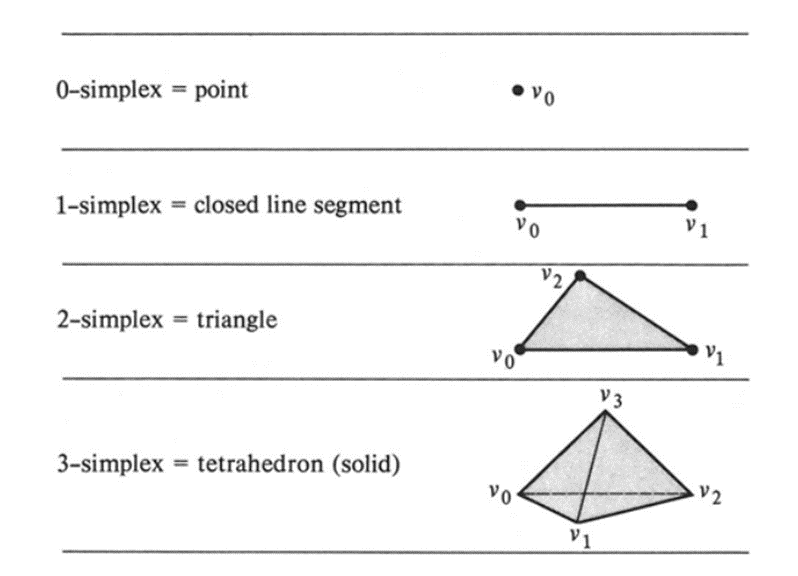
Given  affinely independent points
  , an
, an  -simplex is the smallest convex set containing these points. Formally, it is defined as:
 ![S = [v_0, v_1, \dots, v_n] = \left\{ x \in \mathbb{R}^N \mid x = \sum_{i=0}^{n} \lambda_i v_i, \\ \sum_{i=0}^{n} \lambda_i = 1, \\ \lambda_i \geq 0 \right\}.](https://nhsjs.com/wp-content/ql-cache/quicklatex.com-257d4e277493af49aba7db02b8cdc823_l3.png "Rendered by QuickLaTeX.com")
The points  are called the vertices of the simplex.
Face A face of a simplex  is another simplex formed by a subset of its vertices. Specifically, any simplex
 ![F = [v_{i_0}, v_{i_1}, \dots, v_{i_k}]](https://nhsjs.com/wp-content/ql-cache/quicklatex.com-d6220fbf0aed4a4d28bdfcad94decdc3_l3.png "Rendered by QuickLaTeX.com") with
with  is a face of .
Simplicial Complex
A simplicial complex  is a finite collection of simplices satisfying the following conditions:
Every face of a simplex in is also in .
The intersection of any two simplices in is either empty or a face of both simplices.
Triangulation
A triangulation of a topological space  consists of a simplicial complex and a homeomorphism
  .
.
Triangulation is important in simplicial homology because it underscores the essential process behind redefining a topological space into a simplicial complex, which makes it possible for the calculation of homology groups to be carried out.
Formal Algebraic Formulation of Homology Groups
We now introduce the algebraic framework necessary to define and calculate homology groups.
Given a simplicial complex , the -th chain group  is the free abelian group generated by the oriented -simplices of . Elements of are formal sums of the form:

where  and
and  are oriented -simplices.
The boundary operator  is a group homomorphism defined on an oriented -simplex
 ![[v_0, v_1, \dots, v_n]](https://nhsjs.com/wp-content/ql-cache/quicklatex.com-7a20bef793f928321753268edc3ba20d_l3.png "Rendered by QuickLaTeX.com") as:
as:
![\partial_n ([v_0, \dots, v_n]) = \sum_{i=0}^{n} (-1)^i [v_0, \dots, \hat{v}_i, \dots, v_n],](https://nhsjs.com/wp-content/ql-cache/quicklatex.com-252ef8e5a34cc8e8ec67ee8adf3879cf_l3.png "Rendered by QuickLaTeX.com")
where  indicates that the vertex is omitted.
Orientation of simplices is crucial. Swapping two vertices reverses the orientation:
![[v_0, v_1, \dots, v_n] = -[v_1, v_0, v_2, \dots, v_n].](https://nhsjs.com/wp-content/ql-cache/quicklatex.com-79dbc3487de4fd013c0e13059775d05f_l3.png "Rendered by QuickLaTeX.com")
The boundary operator formalizes the intuitive notion of finding the boundary for a simplex. For example, intuitively the boundary of a triangle, which is a  -simplex would be the three edges. For the boundary operator, we see that the boundary would be calculated to be the sum of the three
  -simplices, which represents the edges.
For any , the composition of boundary operators satisfies  .
.
We need to verify that applying the boundary operator twice to any element of yields zero. Consider an oriented -simplex . Applying  gives:
![\[\partial_n([v_0, \dots, v_n]) = \sum_{i=0}^n (-1)^i [v_0, \dots, \hat{v}_i, \dots, v_n].\]](https://nhsjs.com/wp-content/ql-cache/quicklatex.com-fce224df12389f9ae6326536b8894ac2_l3.png "Rendered by QuickLaTeX.com")
Applying  to each term:
![partial_{n-1}(\partial_n([v_0, \dots, v_n])) = \sum_{i=0}^n (-1)^i \partial_{n-1}([v_0, \dots, \hat{v}_i, \dots, v_n]).](https://nhsjs.com/wp-content/ql-cache/quicklatex.com-f6286b49a8ddd5ab469a35f4888552b0_l3.png "Rendered by QuickLaTeX.com")
Each term ![\partial_{n-1}([v_0, \dots, \hat{v}_i, \dots, v_n])](https://nhsjs.com/wp-content/ql-cache/quicklatex.com-887b185a6155fa9e2ad491c064690b36_l3.png "Rendered by QuickLaTeX.com") is a sum of
is a sum of  -simplices with appropriate signs. When we sum all these terms, each -simplex appears twice with opposite signs due to the alternating sign in the definition, resulting in a total sum of zero. Therefore, .
This property ensures that boundaries of boundaries are always zero which makes sense geometrically as a boundary would cycle back to itself and its boundary would be zero.
The -th homology group of a simplicial complex is defined as:

In this context:
 consists of -chains whose boundary is zero, called -cycles.
 consists of -chains that are the boundary of some
  -chain, called -boundaries.
Thus, intuitively one can interpret the homology group  as denoting all the -dimensional “holes” in the simplicial complex . An equivalence class of cycles in is known as the homology class. Informally, each homology class would correspond to one -dimensional “holes”.
We know that the homology group can be used to detect multidimensional “holes” in any topological space. However, when we are working with raw point cloud data in  , we face a major problem due to the lack of connectivity between data. A method to bypass this is to build a Vietoris-Rips complex.
Vietoris-Rips Complex
Given a set of points  , we choose a parameter
  . The Vietoris–Rips complex
  contains a simplex
 ![[p_{i_0}, \dots, p_{i_n}]](https://nhsjs.com/wp-content/ql-cache/quicklatex.com-35b60ac04e5002d5f32e945a2b05536e_l3.png "Rendered by QuickLaTeX.com") if and only if all pairwise distances between these points are at most
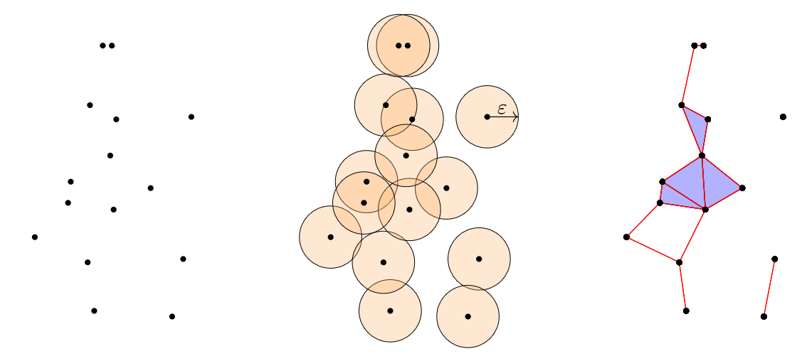
if and only if all pairwise distances between these points are at most  . Alternatively, one can imagine drawing balls of radius
  around each point; whenever a group of points has pairwise intersecting balls, we include the corresponding simplex in . See Figure 2.
Vietoris-Rips Complex Let  and
and  . The Vietoris–Rips complex is a simplicial complex with vertex set , and a subset
  is an -simplex of
Persistent Homology
Persistent Homology is a method to compute topological features for spaces with multiple scales. This technique is adopted from algebraic topology and, more specifically, homology theory. We will properly explain the theory of persistent homology here.
Filtration A filtration of a simplicial complex is a family of subcomplexes
![\[ \{K_t\}_{t\in T}, \quad t_0 < t_1 < \cdots < t_n, \]](https://nhsjs.com/wp-content/ql-cache/quicklatex.com-8ab600b5d376d60ab3620f6899f9fd52_l3.png "Rendered by QuickLaTeX.com")
such that
![\[ \emptyset = K_{t_0} \subseteq K_{t_1} \subseteq \cdots \subseteq K_{t_n} = K. \]](https://nhsjs.com/wp-content/ql-cache/quicklatex.com-e6b21810d6dacb85ae7c227be1550e2d_l3.png "Rendered by QuickLaTeX.com")
In a point-cloud context,  is the Vietoris–Rips complex at scale
  .
.
Each inclusion map  (for
(for  ) induces a map on homology:
![\[ i_{i,j} : H_n(K_{t_i}) \;\longrightarrow\; H_n(K_{t_j}). \]](https://nhsjs.com/wp-content/ql-cache/quicklatex.com-cce8615bcf74bc473990859ee39487d6_l3.png "Rendered by QuickLaTeX.com")
Persistent Homology Group For , the -th persistent homology group is defined by 
In other words,  includes all homology classes that appear by or before
  and that remain non-trivial at least until
  .
.
Birth and Death of Homology Class We say a -dimensional homology class  is born at
  if is nontrivial in
  and was trivial in
  for all
  . Similarly, we say that a homology class dies at
  if remains nontrivial for all thresholds
  and becomes trivial in
  for all
  . If a class never dies within the range considered of , we conventionally set
  . The main way to visualize birth-death information is via the persistence diagram.
Persistence Diagram A persistence diagram in dimension is a multiset of points in the plane  . Each homology class that appears in the filtration is represented by a point
  , where
  and
and  are the birth and death of .
Methods
We used a total of 461 MRI images from a Kaggle OASIS data set, categorized into four distinct classes: Non-Demented, Very Mild Demented, Mild Demented, and Demented. The Kaggle data set did not disclose any personal information about the participants to protect their privacy. The severity classification is based on the provided data and also the Clinical Dementia Rating (CDR) scores. Of the 461 subjects, 230 were labeled Non-Demented (cognitively normal), 77 Very Mild Demented, 73 Mild Demented, and 81 Demented. Table 1 summarizes the class distribution. This imbalance (with the majority class being Non-Demented and the minority class Demented) may introduce significant bias. Therefore, we will address potential class imbalance by using stratified sampling in our data splits and by applying class-weighted loss functions during model training (assigning higher weight to underrepresented classes).

This Kaggle set is a publicly available version of the OASIS-1 MRI dataset9.The MRI data (NiFTI files) were converted into 2D JPEG images along the axial ( ) axis. Each 3D volume was divided into 256 slices; slices from index 100 to 160 (approximately 60 slices per subject) were selected for analysis, as these central slices contain the most relevant brain structures. We then conducted intensity normalization on the selected slices to scale voxel intensities into
 ![[0,1]](https://nhsjs.com/wp-content/ql-cache/quicklatex.com-a4825a08c7bb8da4e97b285db8754278_l3.png "Rendered by QuickLaTeX.com") . We attempted to experiment with Gaussian smoothing (with
. We attempted to experiment with Gaussian smoothing (with  ) to reduce high-frequency noise; however, this preprocessing step had a negligible impact on the topological features, so it was omitted from the final pipeline for simplicity.
Persistent Homology Feature Extraction
After preprocessing, the next step was topological feature extraction via persistent homology. Every 2D slice can be viewed as a topological space (a grayscale intensity function defined on a 2D grid of pixels) where pixel intensities represent scalar values on that domain. We constructed a Vietoris–Rips (VR) filtration on the set of pixels, treating pixel coordinates as points with an intensity-based inclusion criterion. Specifically, for a given intensity threshold , we include all pixels with intensity  and consider their spatial arrangement: each such pixel is treated as a point in . We build a VR complex on these points using the Euclidean distance between pixel coordinates as the metric. As the threshold decreases from 0 to 1, more pixels are added and the VR complex grows. We sampled 100 linearly spaced intensity thresholds between
  and
and  . The distance threshold for the Rips complex at each step was gradually increased (from 0 up to the image’s diagonal length) to ensure connectivity; at the final intensity threshold
  , all brain pixels are included and eventually all components merge into one, ending the filtration. At each threshold, one observes the appearance or merging of topological features: connected components, loops, or voids corresponding to 0-dimensional, 1-dimensional, or 2-dimensional homology classes, respectively. These events give rise to persistence diagrams (PDs) that summarize the birth and death scales of every topological feature throughout the filtration process. In our context, the 0-dimensional homology classes (
 ) correspond to connected components of bright regions in the slice (which appear as separate islands at high thresholds and merge as the threshold lowers), and the 1-dimensional classes (
 ) correspond to loops (enclosed voids or cavities that form around darker regions such as ventricles or sulci as the space fills in). We restricted our computation to and (connected components and loops) because 2-dimensional holes (
 ) do not appear in 2D image data, which also helped reduce computational load. We used the Ripser library for efficient VR persistence computation. Additionally, we also filtered out short-lived topological features, whose persistence is less than 5 voxels in intensity units, as these were likely noise.
Although for 2D image data one could use a cubical complex (treating each pixel and its 8-neighbors as a grid complex), a method which is more computationally efficient, we decided to choose the Vietoris–Rips complex for compatibility with our pipeline and prior implementations. We acknowledge that cubical complexes offer significant speed benefits for pixel data and plan to evaluate such alternatives in future work.
For each 2D slice, we computed separate persistence diagrams in dimensions  and . We then needed to aggregate the information from a subject’s multiple slices into a single feature vector. We achieved this by using persistence images as a vectorization of the persistence diagrams (H. Adams, T. Emerson, M. Kirby, et al. Persistence images: a stable vector representation of persistent homology. Journal of Machine Learning Research 18(8), 1–35 (2017).). In brief, a persistence image is a summarized representation where each point in a persistence diagram is mapped to a Gaussian kernel on a discrete grid, and the contributions are summed. In our implementation, we first combined all persistence diagram points from the 60 slices of a subject (treating the collection of that subject’s and points as one large set). We then defined a
  grid over the birth-death plane and placed a Gaussian bump (with standard deviation
  in normalized intensity units) at the coordinates of each persistence point; the intensities of overlapping Gaussians were summed. The result is a persistence image encoding the distribution of persistent topological features for that subject. This image was then flattened into a vector to serve as the input features for classification. This approach replaces the earlier method of slice-wise diagram summation with a standardized and more reproducible vectorization of a persistent homology. Note that in our current aggregation, all slices were weighted equally; this uniform weighting may introduce noise since not every slice carries equal diagnostic information. In future work, we plan to explore weighting slices (or selecting a subset of key slices) based on anatomical regions of interest (for example, giving more weight to slices that intersect the hippocampus or ventricles) to further enhance the persistence-based features.
Following the extraction of topological features, we trained two conventional machine learning models on the persistence image vectors: a regularized multivariate logistic regression (with  regularization to avoid overfitting) and a random forest classifier. The logistic regression model served as a simple baseline, while the random forest (with 100 decision trees by default) could exploit non-linear interactions among topological features. We performed a grid search with cross-validation (10-fold within the training set) to tune key hyperparameters for these models, such as the regularization strength in logistic regression and the maximum tree depth and number of trees in the random forest. (The chosen random forest used 100 trees and a maximum depth of 10, based on validation performance.)
CNN Architecture and Training
In parallel to the persistence-based approach, we developed a deep CNN to serve as a benchmark on the raw image data. We used an architecture inspired by the AlexNet model, similar to the design by Fu’adah et al10. for AD classification. Our CNN consisted of three convolutional layers (with 3×3 filters) each followed by a ReLU activation and a max-pooling layer. The numbers of feature maps in these layers were 32, 64, and 128, respectively. After convolution and pooling, the network included two fully connected layers with 128 and 64 neurons, respectively. We applied a dropout of 0.5 after the first fully connected layer to reduce overfitting. The final output layer was a softmax classifier that produced probabilities for each of the four AD severity classes. This architecture is relatively compact to mitigate overfitting given the data size, while still deep enough to learn meaningful spatial features.
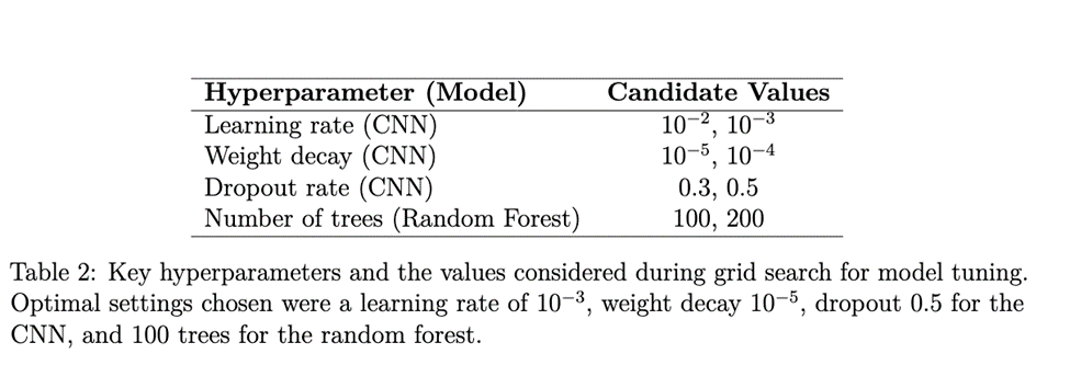
We trained the CNN on the same set of subjects (using their stack of slices as input). To aggregate slice-level predictions into an overall subject-level classification, we employed a simple strategy: the CNN produced a prediction for each 2D slice, and these were averaged across the 60 slices of a subject to yield the subject’s predicted class (effectively a majority vote/mean probability approach). We augmented the training data with random rotations, flips, and translations of slices to artificially increase data diversity. The network was trained using a cross-entropy loss and optimized with the Adam optimizer. We split the data into 70% training, 15% validation, and 15% test sets, using stratified sampling (with a fixed random seed = 42) to ensure each split maintained the class proportions from the full dataset. All model selection (e.g., early stopping and hyperparameter tuning) was done on the training/validation sets, with the test set held out for final evaluation. We conducted five independent runs with different random weight initializations to assess robustness. Key hyperparameters for the CNN (learning rate, weight decay, dropout rate) and for the random forest (number of trees) were tuned via grid search on the validation set. Table 2 lists the hyperparameter search space explored.
In an exploratory experiment, we also constructed a hybrid model that combines deep learning with persistent homology features. In this approach, we took the feature vector from the CNN’s penultimate layer (the 64-dimensional output of the last fully connected layer before softmax) and concatenated it with the 400-dimensional persistence image vector for each subject. A simple feed-forward classifier (a single hidden layer of 64 neurons with ReLU, then softmax) was trained on this combined representation. This hybrid model achieved a slightly higher accuracy than either model alone (Table 3), suggesting that the persistence-based features provide complementary information to the CNN. However, for the focus of this research paper, our primary analysis is centered around comparing pure topological method classifiers to pure CNN.
Ethical Considerations
All the images are from the OASIS project, which is publicly available. All patient’s information is anonymous, and all data used are in accordance with the OASIS data usage policies. Our secondary analysis did not require further institutional review as the data do not contain identifiable personal information.
Results and Discussions
The classification performance for the three classifiers is shown in Table 3. In particular, the random forest classifier achieved the highest overall accuracy of 91.8%, followed by CNN (86.5%) and logistic regression (78.2%). The CNN accuracy graph is shown in Figure 4.
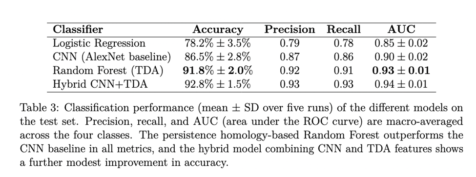
The model performance for the three individual classifiers and the hybrid model is shown in Table 3. In particular, the random forest classifier using persistence image features achieved the highest overall accuracy of 91.8%, followed by the CNN (86.5%) and logistic regression (78.2%). The random forest also attained an averaged area under the ROC curve (AUC) of approximately 0.93, indicating excellent discrimination capability. Figure 4 shows the CNN’s training and validation accuracy curves over epochs.

A one-way ANOVA on the accuracies of the three main classifiers yielded an  statistic of 55.32 (with
  ). Post-hoc Tukey’s HSD tests indicated that each pair of models had a significant difference in mean accuracy, where the random forest classifier is statistically superior compared to the logistic regression and CNN. To further validate the performance gap, we also conducted a McNemar’s test comparing the CNN and the persistence-based classifier’s output labels, which was significant (
 ), and a paired -test on accuracy across the five repeated runs (
 ). These statistical tests reinforce that the inclusion of topological features provides a real performance benefit. Over five random train/test splits, the random forest’s accuracy was
  , indicating the model is reasonably stable and suggesting a 95% confidence interval roughly in the range
 ![[89.5%, 93.5%]](https://nhsjs.com/wp-content/ql-cache/quicklatex.com-271e4e274b2ccec359074f2be79368fb_l3.png "Rendered by QuickLaTeX.com") for its accuracy.
for its accuracy.
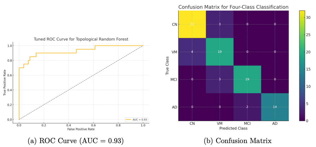
We also evaluated the models in terms of their ROC curves and confusion matrices for more detailed insights. Figure 5a shows the ROC curve for our topological random forest classifier. The curve hugs the upper-left corner, and the AUC of 0.93 reflects that the model achieves a high true-positive rate for a given false-positive rate. Figure 5b presents the confusion matrix for the four-class classification on the test set. Most misclassifications occurred between adjacent severity categories (e.g., Very Mild vs. Mild), which is expected. The model was especially accurate at distinguishing the endpoints: Non-Demented vs. Demented. In fact, for distinguishing cognitively normal versus demented subjects, the model’s sensitivity was about 88% and specificity about 95%. This suggests that the topological features are capturing patterns strongly indicative of severe disease while occasionally confusing intermediate stages.
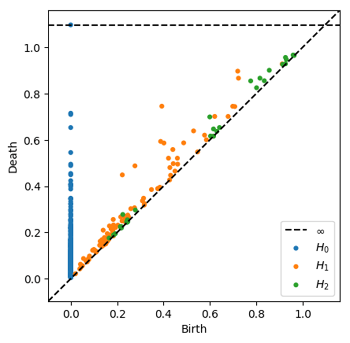
Beyond overall performance metrics, we examined the actual learned topological patterns distinguishing the classes. Figure 6 displays persistence diagrams for three subjects: a cognitively normal (Non-Demented) control, an MCI case (combining Very Mild/Mild Demented), and an AD patient (Demented). Each diagram plots the persistence of topological features (with features shown as blue points and features as orange triangles). We observe qualitative differences: the AD persistence diagram (Figure 6c) contains several features with long lifetimes (points farther from the diagonal) in both and , indicating the existence of prominent topological structures such as large voids corresponding to enlarged ventricles or pronounced separations of tissue due to cortical thinning. The cognitively normal case (Figure 6a) tends to have most features concentrated near the diagonal which have shorter lifetimes, showing that the brain structure is more topologically “connected” and homogeneous when thresholded. The MCI case (Figure 6b) lies in between, showing moderate persistence features. These visualizations help confirm that our persistence-based features align with known anatomical changes: as the disease progresses, one can see an increase in long-lived topological features, consistent with greater atrophy and structural disintegration in the brain.
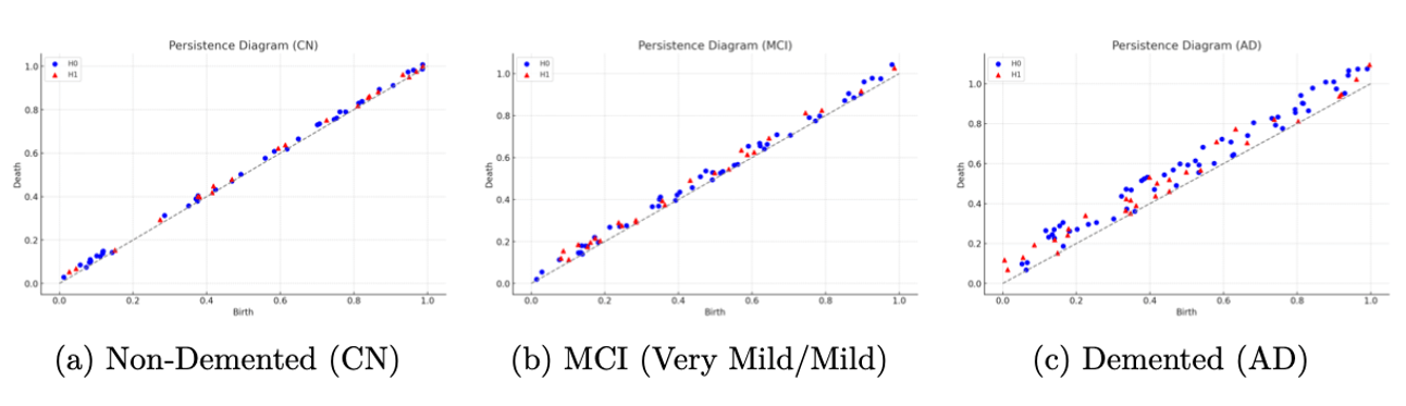 (connected components) and orange triangles for (loops), plotted at coordinates (birth threshold, death threshold). Features near the diagonal have short lifetimes, while those farther away are longer-lived. The AD case (c) exhibits several long-lived features (e.g., orange triangles far from diagonal), indicating persistent loops/voids consistent with enlarged ventricles and pronounced cortical atrophy. The cognitively normal case (a) has features mostly with brief persistence (clustered near the diagonal), reflecting a more topologically cohesive brain structure.
We also analyzed which topological features were most important for the random forest classifier’s decisions. Figure 7 plots the top ten feature importance scores from the random forest averaged for all trees. The two most important features were the maximum lifetime and the number of features above a certain persistence threshold, respectively. Intuitively, this suggests that having a large connected component persist for a long range of intensity thresholds and the overall count of significant loops were key discriminators. These correspond to anatomical observations that a very large lifetime might occur if one brain region remains isolated until a low threshold, and numerous loops could indicate complex patterns of holes in diseased brains. Other important features included the total persistence in and , further emphasizing that the overall “topological signal” differentiates the classes. This feature importance analysis increases the interpretability of the model as the most predictive variables are linked with the topological characteristics of the MRI data.
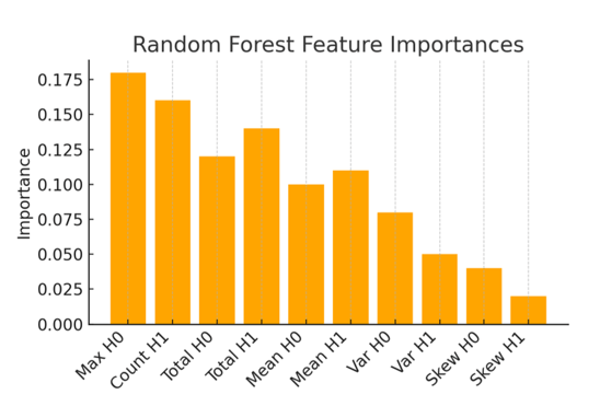 feature (connected component persistence) and the count of loops with high persistence. These features align with known AD-related changes: for example, a large lifetime might correspond to a region of the brain (such as a ventricle) that remains topologically separate until a low threshold, indicating significant tissue loss, and a high count of loops reflects more numerous voids or cavities in the brain structure.
Limitations: Despite encouraging results, our study has several limitations.
- First, the sample size is modest, which may limit generalizability. The model could overfit subtle features of this dataset despite our cross-validation and regularization efforts. Testing on an independent cohort from a different demographic or scanner will be important to ensure the result generalizes.
- Second, our analysis was based on 2D slice data rather than the full 3D MRI volumes. While aggregating multiple slices captures some 3D information, it does not fully leverage spatial continuity across slices. A truly volumetric 3D persistent homology approach could potentially improve performance by capturing patterns that span across adjacent slices, at the cost of increased computational complexity. We plan to explore applying persistent homology to 3D brain volumes in future work to better exploit the rich structural information in MRI data.
- Third, while we introduced interpretability via topological features, the method still ultimately relies on statistical learning and could be affected by confounding factors. For instance, if the AD group systematically had slightly lower image quality or a particular preprocessing artifact, the persistent homology might pick that up rather than true anatomical differences. We tried to minimize such biases through careful preprocessing and by including only well-matched cases, but this risk remains.
- Fourth, our persistent homology analysis focused on structural MRI intensity topology; however, other data modalities or TDA strategies might capture additional information. We did not incorporate functional MRI or diffusion MRI, which could contain complementary topological signatures of functional brain networks or white matter tract integrity in AD. Additionally, our current pipeline computes persistent homology on the many slices of the entire brain; a more targeted approach might examine specific regions (like the hippocampus or ventricles) to reduce noise and enhance sensitivity to localized changes. Another limitation is the computational complexity of persistent homology for high-resolution images. Although we optimized the process by restricting it to and and also using software optimizations, computing persistence on full 3D volumes or very large images can be slow for larger datasets or higher homology dimensions. Fortunately, ongoing advances in TDA algorithms and hardware are continually improving feasibility. In practice, one might also consider downsampling images or focusing on extracted surfaces to simplify the topology computation.
Demographic Fairness Considerations: We acknowledge the importance of evaluating demographic fairness in clinical AI models. Bias can arise if a model performs differently across demographic subgroups such as sex or ethnicity11. In our dataset, the proportion of females vs. males and the distribution of ages were roughly similar between diagnostic groups. We conducted a preliminary subgroup analysis. We found that the model’s accuracy for male versus female subjects differed by less than 2% on the test set, and similarly, no large disparity was observed when comparing younger vs. older subjects (using the median age to split). However, our sample of non-Caucasian participants was very small, reflecting the OASIS cohort’s lack of diversity. This precludes any meaningful analysis by ethnicity and could hide biases. Recent work on AD prediction models has found that even when overall accuracy is high, fairness metrics may not be satisfied. Although our data did not allow a thorough fairness evaluation, we stress that this is an important issue. In a clinical deployment, the model should be tested on more diverse populations. Techniques such as re-sampling or adding fairness constraints during training could be applied to mitigate bias. We have included this discussion to prompt awareness and future investigation into the fairness of TDA-based diagnostic tools.
Outlook and Future Work: This work provides several paths for future research. One very promising direction is to develop hybrid models that combine both deep learning and TDA. Our preliminary experiment with a hybrid model (concatenating CNN features and persistence features) hinted at a slight improvement (Table 3), and recent studies suggest that topological features can indeed enhance neural network classifiers12. A more sophisticated fusion could involve injecting persistence features into intermediate layers of a network or designing a neural architecture that computes topological summaries as part of its structure. For example, one could imagine a multi-branch model where one branch is a CNN processing the raw images and another branch computes a persistence-based feature map, with the two merged for a final decision. Such approaches might yield even higher accuracy while retaining interpretability.
Furthermore, applying TDA to other aspects of AD is an interesting future direction. For instance, analyzing longitudinal changes in persistence diagrams could quantify disease progression over time. Also, extending persistent homology to functional connectivity networks (from fMRI or EEG) or multimodal data could provide complementary information beyond structural MRI alone. Integrating multimodal data within a topological framework might uncover complex relationships that elude standard models.
Finally, we emphasize the need to validate and refine our model based on a broader and larger datasets. Of course, gaining access to the entire dataset from OASIS would be a great first step into improving the reliability and applicability of the model in real world scenarios. By addressing these limitations and exploring the outlined future directions, we hope to move closer to the clinical deployment of TDA tools that aid in the early detection and understanding of Alzheimer’s disease.
Conclusion
We presented an application of topological data analysis for Alzheimer’s disease diagnosis using MRI data. By leveraging persistent homology, our approach extracts robust topological features that characterize differences between AD and healthy brains. The proposed TDA-based model achieved accuracy and AUC a little lower compared to the accuracy of the state-of-the-art deep CNN models, while providing more interpretable results linked to known anatomical changes in AD. Overall, the encouraging results and insights obtained suggest that topological features capture meaningful structural biomarkers of AD. We envision that continued refinement of this approach—especially in combination with deep learning and evaluation on more diverse test subjects—will pave the way for more effective and successful tools for AD diagnosis and severity classification.
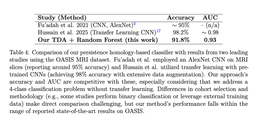
In comparison to other approaches on similar data, our model’s performance is competitive. Table 4 highlights metrics from two recent studies that applied deep learning to the OASIS MRI dataset. Fu’adah et al achieved about 95% accuracy using an AlexNet-based CNN, and Hussain et al. reported 98% accuracy by fine-tuning pre-trained CNN models (transfer learning). Our persistence-based model’s accuracy (91.8%) and AUC (0.93) are in a similar range. It should be noted that direct comparisons can not be made abruptly. For example, Hussain et al. combined OASIS with additional data and tackled a slightly different classification setup, while my machine learning model had access to a limited amount of data from OASIS. Moreover, some reports in literature pertain to binary classification (AD vs. CN) rather than classifying into four different classes. Nonetheless, the fact that our TDA approach approaches the performance of pure CNN models is encouraging. It suggests that topological features can provide a powerful alternative to deep learning, with the added benefit of interpretability. By integrating TDA with machine learning, as we have done, researchers may gain new perspectives on the data—identifying not just what the model predicts, but why, in terms of brain structure differences. We plan to further refine this approach and test it against other state-of-the-art methods on larger and more diverse datasets to fully establish its efficacy.
References
- H. Edelsbrunner, D. Letscher, A. Zomorodian. Topological persistence and simplification. Discrete & Computational Geometry 28, 511–533 (2002). [↩]
- Alzheimer’s disease fact sheet. https://www.nia.nih.gov/health/alzheimers-and-dementia/alzheimers-disease-fact-sheet (2023). [↩]
- L. Kuang, D. Zhao, J. Xing, Z. Chen, F. Xiong, X. Han. Metabolic brain network analysis of FDG-PET in Alzheimer’s disease using kernel-based persistent features. Proceedings of the 2020 IEEE International Conference on Bioinformatics and Biomedicine (BIBM), 1202–1207 (2020 [↩]
- J. Xing, J. Jia, X. Wu, L. Kuang. A spatiotemporal brain network analysis of Alzheimer’s disease based on persistent homology. Frontiers in Aging Neuroscience 14, 788571 (2022). [↩]
- Y. N. Fu’adah, H. F. R. Dewi, M. Mutiarin, I. K. E. Purnama. Automated classification of Alzheimer’s disease based on MRI image processing using convolutional neural network (CNN) with AlexNet architecture. Journal of Physics: Conference Series 1844, 012020 (2021). [↩]
- M.A. Armstrong. Basic Topology (1983). [↩]
- T. Gowdridge, N. Dervilis, K.Worden. On topological data analysis for structural dynamics: an introduction to persistent homology. https://doi.org/10.48550/arXiv.2209.05134 (2022). [↩]
- Understanding the shape of data (II). https://quantdare.com/understanding-the-shape-of-data-ii/ (2019). [↩]
- Kaggle. OASIS Brain MRI dataset. https://www.kaggle.com/datasets/ninadaithal/imagesoasis (2021). [↩]
- Y. N. Fu’adah, H. F. R. Dewi, M. Mutiarin, I. K. E. Purnama. Automated classification of Alzheimer’s disease based on MRI image processing using convolutional neural network (CNN) with AlexNet architecture. Journal of Physics: Conference Series 1844, 012020 (2021). [↩]
- J. Yuan, K. A. Linn, et al. Algorithmic fairness of machine learning models for Alzheimer disease progression prediction. JAMA Network Open 6(11), e234049 (2023). [↩]
- M. D. Prata Lima, G. A. Giraldi, G. Miranda. Image classification using combination of topological features and neural networks. https://doi.org/10.48550/arXiv.2311.06375 (2023). [↩]


