Testing Machine Learning Algorithms on Cervical Cancer Dataset

Abstract

Cervical cancer is one of the most common cancers affecting women worldwide, with the highest incidence rates found in low- and middle-income countries. Although it can affect women of various ages, it is most frequently diagnosed in those aged 30 years or older. In regions with limited healthcare infrastructure, many women are diagnosed in later stages due to insufficient access to early screening and diagnosis. Early risk detection is essential for improving outcomes and reducing treatment costs. Machine learning (ML) algorithms have emerged as valuable tools to support, rather than replace, standardized early detection methods such as Pap smears and Human Papillomavirus (HPV) testing. These algorithms can assist medical professionals by identifying individuals at higher risk, helping prioritize care, and potentially confirming clinical findings. ML models can process large volumes of patient data efficiently, enabling more timely and informed decision-making. This study evaluates several machine learning algorithms to determine their effectiveness in supporting cervical cancer risk assessment. Performance is measured using key metrics such as accuracy, sensitivity, specificity, and Area Under the Receiver Operating Characteristic curve (AUROC). Among the models tested, Support Vector Machine (SVM) and Light Gradient Boosting Machine (LightGBM)achieved the highest overall performance across all metrics, making them most promising for early risk detection. A detailed analysis is conducted on these promising algorithms, highlighting both their advantages and limitations in a real-world healthcare context. Extensive discussion on all algorithms clinical potential, limitations, and implications for future integration into healthcare settings is also performed.

Keywords: Cervical Cancer, Early Detection, Machine Learning Algorithms 

Introduction

Cervical cancer is the fourth most common cancer in women globally, preceded by breast cancer, colorectal cancer, and lung cancer¹. HPV is a sexually transmitted disease that affects the genitals and other areas, and normally, most sexually active people are infected by it at least once in their lifetime¹. Usually, the immune system can clear HPV from the body, but untreated persistent HPV diseases in the cervix, the lower part of the uterus, cause 95% of reported cervical cancers¹. Cervical cancer usually develops slowly over time, normally 15-20 years¹, but women with weaker immune systems can develop cancerous cells in 5-10 years¹. 

Diagnosis for cervical cancer is most frequently found in women ages between 35 and 44 in America². It is rarely found in women under 20². Cervical cancer rarely occurs in women who have been regularly tested and screened for cervical cancer before 65². 

The advancement of effective methods for both the prevention of cervical cancer and the treatment of cervical cancer decreases overall cervical cancer cases. Cervical incidence rates decreased more than half from the mid-1970s to the mid-2000s, and have stabilized since². Adequate prevention and treatment, however, primarily exist in developed countries. For most developing countries, the equipment needed to take precautionary measures like HPV vaccines or successful treatment may not be readily available. This allows for many cervical cancer cases to go unnoticed and progress. In 2022, there were 660,000 new cases of cervical cancer worldwide¹. In that same year, there were also around 350,000 cervical cancer deaths, 94% of which occurred in low and middle-income countries¹. 

Treatment of cervical cancer is expensive and usually pertains to a patient undergoing surgery or therapy to remove the cancerous cells. Especially in developing or poor countries, people may not have enough money to cover treatment costs. In 2020, the cost of cervical cancer care was 2.3 billion dollars, with the average per-patient costs for medical services for the end-of-life phase being $97,000, followed by the initial care phase ($58,700) and continuing care phase ($4,000)³. Precautionary measures are a much more effective and affordable approach, especially with the introduction of risk prediction models that contain machine learning algorithms². 

Machine learning algorithms work by taking in data that contains risk factor information like age, and smoking status, and use the data to make an accurate prediction of cervical cancer presence. Machine learning algorithms achieve this by training on data that contains risk factor data on an individual, and if there was a presence of cervical cancer in the patient or not. From this, the algorithms use their unique properties to predict a pattern to then evaluate on a testing data set⁴. 

Each algorithm varies differently from the other, specifically in how they arrive at a prediction. Because of this, certain algorithms will perform more accurately and efficiently in some datasets than others. This study aims to determine which algorithm chosen for this study shows the most effective results on a cervical cancer dataset. The algorithm will be chosen through comparison of accuracy, metrics such as specificity, sensitivity and AUROC, and finally with visualizations such as AUROC curve and confusion matrices.

Literature Review

Shetty et al. compared several machine learning models such as Decision Tree and K-Means across different studies⁵. Despite the varied approaches taken in those studies, a common issue highlighted was data imbalance—especially in image-based datasets—and the importance of addressing it properly. This study also focuses on comparing key machine learning algorithms, applying a consistent method across all models to avoid evaluation bias. While this improved the fairness of comparison, data imbalance still posed challenges despite efforts to reduce it. Shetty et al. noted that SVM was widely used and effective in handling overfitting and bias, but suffered from long computation times and lack of transparency. In contrast, computation times were kept manageable in this study, and feature importance analysis was used for LightGBM, the top-performing model, to improve interpretability and support its performance. Parikh et al. experienced similar limitations⁶. Their work involved testing Decision Tree, Random Forest, and K-Nearest Neighbor models, and they attempted to reduce bias in the data by simplifying the dataset. This helped to some extent, but led to a trade-off between result quality and model performance. Some columns still contained bias that couldn’t be fully addressed. In this study, similar issues were encountered—Synthetic Minority Oversampling Technique (SMOTE) was used to reduce class imbalance, but some inherent bias in the dataset remained. Unlike Parikh et al., feature selection algorithms were not applied, which might have improved model performance further. However, hyperparameter tuning and a three-way data split (training, validation, testing) were used to help manage overfitting. Although k-fold cross-validation was not included, its benefits are acknowledged and it remains a potential method for enhancing the reliability of results in future research.

Suman et al. trained and tested Random Forest, Neural Network, Support Vector Machine, AdaBoost, Bayes Net, and Decision Tree algorithms using biopsy data from 858 patients at Hospital Universitario de Caracas⁷. Their use of k-fold cross-validation strengthened the reliability of their results, with Bayes Net achieving the highest accuracy at 96.38%. However, the study did not clearly outline how missing values were handled, which is a notable gap. In contrast, this study ensured all missing values were addressed through preprocessing steps to avoid bias during model training. While k-fold validation was not implemented here, its value is recognized, and it remains a candidate for future experimentation.

Yang et al. similarly applied k-fold cross-validation when developing Multilayer Perceptron (MLP) and Random Forest models to evaluate diagnostic accuracy⁸. Random Forest was also used to rank risk factors through an importance index. This aligns with the current study’s use of feature importance analysis on the best-performing model (LightGBM), supporting a growing emphasis on interpretability. Like Yang et al., this project also faced limitations from dataset size, which contributed to challenges with overfitting despite mitigation strategies such as SMOTE and validation splitting.

Nithya et al. focused primarily on feature selection, experimenting with methods like Recursive Feature Elimination, the Boruta algorithm, and Conditional Inference Trees in combination with models like Random Forest⁹. Their work showed that thoughtful feature selection improved accuracy, reduced overfitting, and improved model efficiency. This study did not incorporate advanced feature selection algorithms, opting instead for a standardized feature set across models for consistent comparison. However, the potential value of integrating such methods is acknowledged, especially in improving generalization.

Alsmariy et al. developed an ensemble model combining multiple algorithms, supported by preprocessing steps like SMOTE, Principal Component Analysis (PCA), and feature selection, alongside cross-validation¹⁰. The ensemble approach helped address small dataset size and overfitting concerns. Similarly, this study utilized SMOTE to handle class imbalance and reduce bias in training. However, ensemble methods were not explored here, as the focus remained on comparing individual models directly. The use of PCA and advanced missing value strategies in Alsmariy et al.’s work suggests future directions for improving model robustness in studies with similarly limited datasets.

Tanimu et al. used a Decision Tree model paired with Recursive Feature Elimination and LASSO for feature selection, alongside SMOTEtek—a modified version of SMOTE that also addresses missing data¹¹. Their feature selection and data handling strategies contributed to strong results, including a reported 100% sensitivity. While this study also leveraged SMOTE to combat imbalance, it did not apply advanced feature engineering or SMOTE variants. Nonetheless, model tuning and data preprocessing were used to control for overfitting and improve interpretability. The use of LightGBM, with its built-in handling of missing values and transparent feature ranking, provided an alternative route to similar goals.

Methods

Data

The data used in this research to test the algorithms is found in Kaggle, an online platform for data science sharing¹². The data originally was obtained from ‘Hospital Universitario de Caracas’ in Caracas, Venezuela of which consisted of 858 patients.

The file contains a list of risk factors for cervical cancer leading to a biopsy examination. The risk factors included 24 features of “string data” (transformed into Boolean data for algorithm use) and 12 features of numerical data (either continuous or discrete/integer). For the “string columns” 1 indicated yes and 0 indicated no. The risk factors included age, smoking, Intrauterine Device (IUD), sexual intercourse, STDS, and hormonal contraceptive data, which can all be accessed through the reference section in the paper or in the table below.

Features:	Type:
Age	Integer
Number of Sexual Partner	Integer
First Sexual Intercourse	Integer
Num of Pregnancies	Integer
Smokes	Boolean
Smokes(years)	Continuous
Smokes(packs/year)	Continuous
Hormonal Contraceptives	Boolean
Hormonal Contraceptives(years)	Continuous
IUD	Boolean
IUD(years)	Continuous
STDS	Boolean
STDs(numbers)	Integer
STDs:condylomatosis	Boolean
STDs:cervical condylomatosis	Boolean
STDs:vaginal condylomatosis	Boolean
STDs:vulvo-perineal condylomatosis	Boolean
STDs:syphilis	Boolean
STDs:pelvic inflammatory disease	Boolean
STDs:genital herpes	Boolean
STDs:molluscum contagiosum	Boolean
STDs:AIDS	Boolean
STDs:HIV	Boolean
STDs:Hepatitis B	Boolean
STDs:HPV	Boolean
STDs: Number of diagnosis	Integer
STDs: Time since first diagnosis	Integer
STDs: Time since last diagnosis	Integer
Dx:Cancer	Boolean
Dx:CIN	Boolean
Dx:HPV	Boolean
Dx	Boolean
Hinselmann	Boolean
Schiller	Boolean
Citology	Boolean
Biopsy	Boolean

The following Kaggle repository was expanded to conduct the empirical studies included in the paper¹³. The data was extracted from¹² to build a comprehensive and robust pipeline for training and evaluation of supervised learning methods for the predictive modelling of cervical cancer. Python and Scikit-Learn were used to construct the relevant methods and experiments.

Before training, missing values in the dataset were handled using k-Nearest Neighbors (kNN) imputation with k=2, which estimates missing values based on the average of the two most similar rows. The features were then standardized using StandardScaler to normalize all variables to a comparable scale.

The dataset was split into training (80%) and temporary testing (20%) subsets. The testing subset was further divided evenly into validation (10%) and final test (10%) sets. To address class imbalance in the training set, SMOTE with default parameters was applied.

After the preparation of data, the algorithms Logistic regression, SVM, kNN, eXtreme Gradient Boosting (XGBoost), and LightGBM are imported. The relevant metrics include precision, recall or sensitivity, f1-score, specificity, and accuracy. These were computed using fixed training, validation, and test sets (80/10/10 split), ensuring consistent evaluation across all models. While k-fold cross-validation was not employed, multiple randomized train-test splits were used to ensure result robustness. 

Algorithms 

In this research, we will test the following algorithms: Logistic Regression, SVM, kNN, XGBoost, and LightGBM.
The following algorithms were chosen over deep learning methods like Convolutional Neural Network (CNN) because the data consist of tabular, structured data, rather than image or sequence data. Additionally, classical ML models such as LightGBM and XGBoost are well-suited for mixed-type data, require fewer computational resources, and provide more interpretability.

Logistic regression : Logistic Regression is a linear classification algorithm that models the probability of a binary outcome. It assigns weights to input features (risk factors) and calculates a weighted sum, which is then passed through a function to output a value between 0 and 1, representing the probability of having cervical cancer. The decision boundary is determined by a threshold (usually 0.5).

SVM¹³: SVM is a supervised learning algorithm that constructs a hyperplane (or decision boundary) in a high-dimensional space to separate classes. It finds the optimal decision boundary that maximizes the margin between the closest data points of each class, known as support vectors. 

kNN¹⁴: kNN is a non-parametric, instance-based learning algorithm. It classifies a new data point based on the majority class of its k closest neighbors in the feature space, measured using a distance metric. It uses the training data directly to make predictions.

XGBoost¹⁵: XGBoost is a gradient boosting framework that builds an ensemble of decision trees in a sequential manner. Each new tree is trained to correct the errors of the previous ones by minimizing a loss function. XGBoost includes regularization to prevent overfitting and is known for its efficiency, scalability, and high performance on structured/tabular datasets.

LightGBM¹⁶: LightGBM is an optimized gradient boosting framework similar to XGBoost but with improved speed and lower memory usage. It uses a histogram-based algorithm and grows trees leaf-wise rather than level-wise, which can result in deeper trees and better accuracy. It is particularly efficient on large datasets with many features.

Results

Algorithm:	Median Accuracy:	MedianAUROC:	MedianSpecificity:	Median Sensitivity:
Logistic Regression	0.95	0.97	0.97	0.62
kNN	0.91	0.91	0.97	0.11
SVM	0.97	0.97	0.96	1
XGBoost	0.94	0.97	0.93	0.86
LightGBM	0.96	0.95	0.96	1

The unusually low value of 0.11 in Table 2 corresponds to sensitivity for kNN. This reflects the algorithm’s limited ability to detect positive cases in the context of the highly imbalanced dataset and small sample size. Such outlier results highlight the variability of model performance under challenging data conditions and emphasize the need for cautious interpretation of individual metrics.

Every algorithm could predict the negative class effectively, with high specificity values. The f1-scores and precision values attributed to the negative class were also high. The positive class accuracy, however, varied per algorithm. The two algorithms that performed the best were SVM and LightGBM.

Further comparison between SVM and LightGBM is needed. Thus, the employment of visualizations means of analysis is performed, specifically with confusion matrices and Receiver Operating Characteristic (ROC) curves.

Example random run of SVM 

The figure 1 shows the confusion matrix from one run of the SVM model. Each cell in the matrix represents the number of predictions the model made for each actual class (0 or 1) compared to what it predicted (also 0 or 1).

The diagonal values (from top-left to bottom-right) represent correct predictions, while the off-diagonal values show where the model made mistakes. The color intensity highlights how many predictions fall into each category.

SVM here was able to predict 76/79 negative classes, and predict 4/7 of the positive classes.

This figure shows the ROC curve from a single run of the SVM model. The curve plots how the model’s ability to correctly identify positive cases (True Positive Rate) changes as it also makes incorrect positive predictions (False Positive Rate).

SVM in the ROC curve visualizes obvious variation through the fluctuations with the line, however with an excellent AUROC score of 0.92.

Example run of LightGBM

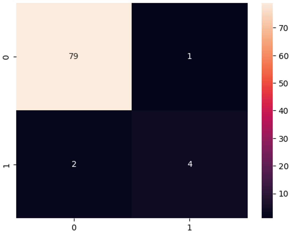
This figure shows the confusion matrix from one run of the LightGBM model. Each cell in the matrix represents the number of predictions the model made for each actual class (0 or 1) compared to what it predicted (also 0 or 1).

The diagonal values (from top-left to bottom-right) represent correct predictions, while the off-diagonal values show where the model made mistakes. The color intensity highlights how many predictions fall into each category.

LightGBM was able to predict 79/80 in the negative class. For the positive class, it was able to predict 4/6.

This figure shows the ROC curve from a single run of the LightGBM model. The curve plots how the model’s ability to correctly identify positive cases (True Positive Rate) changes as it also makes incorrect positive predictions (False Positive Rate).

LightGBM in the ROC curve visualizes less variation compared to SVM due to less fluctuations in the line, and a superior AUROC value of 0.97. Shows consistency of less variation paired with an excellent AUROC score.

Discussion

The most effective algorithms included SVM and LightGBM, with high median accuracy in both positive class and negative class. Both SVM and LightGBM also had solid f-1 scores and specificity values. However, SVM had extremely high variation, with some runs with low positive class recall values and some with 100% positive class recall values. This is evident in the random run used for ROC curve and confusion matrix visualization. LightGBM, on the other hand, was more consistent with less variation. LightGBM performed the most efficiently out of all the algorithms. 

It is likely that LightGBM’s inherent properties contributed to its superior performance. Its unique ability to efficiently handle imbalanced data (a common issue in medical datasets) without requiring extensive tuning could have contributed to its success. Other properties of the algorithm, such as its grading boost mechanism, also likely contributed to its success. Additionally, LightGBM’s support for regularization techniques helps reduce overfitting, making it well-suited for smaller datasets like the one used in this study.

On the other hand, SVM exhibited high sensitivity but displayed significant variance across different runs. Despite the use of SMOTE to balance the dataset, SVM’s variability could still be partly influenced by data imbalance, as oversampling can sometimes lead to overfitting of the minority class. While SMOTE helps prevent the model from ignoring the minority class, the high sensitivity in some cases indicates that SVM might be overly focused on those positive cases, which could lead to issues in generalizing unseen data. Also, although the SVM model achieved a median sensitivity of 1.0, it is important to note that due to the small and imbalanced dataset, some test sets may have contained very few positive samples. This makes the sensitivity metric potentially unstable. Though we employed median reporting to reduce variance, the absence of significance testing or confidence intervals limits the reliability of the performance metrics. Future work will aim to address this through larger datasets and more rigorous statistical analysis. Additionally, while weighted averages offer benefits in representing imbalanced datasets, we prioritized robustness to variance across runs, which median more effectively captures in this case.

Computational time was not an issue in this study, as all times for the algorithms were approximately the same and efficient.

Limitations

Machine learning models for cervical cancer have been developed over various case studies. Methods and ideas previously not available or thought of have developed over time and will continue to be introduced to perfect these models. 

There are still limitations that all researchers face when using algorithms for predictions.

One of the most critical limitations of this study is the nature of the chosen dataset itself—it is both small and highly imbalanced. These characteristics can affect model performance by increasing variance (i.e., performance fluctuates widely between runs) and introducing bias, especially toward the majority class. As a result, metrics like sensitivity and specificity may be less reliable. While SMOTE was applied to address imbalance, and repeated runs were used to smooth variability, these steps cannot fully overcome the limitations of the data. For this study, there isn’t the privilege to connect to hospitals for unique data so the only way to gather data is from public data on the internet. Data availability however in the internet is extremely small, which can in turn impact model efficiency. Limited data can lead to overfitting, which is a deficiency that occurs when a model performs poorly on tested data. Overfitting, in general, is unavoidable but will be countered by testing each algorithm multiple times.
The median values of accuracy, AUROC, sensitivity, and specificity were chosen to reduce the effect of extreme values from repeated runs, particularly due to variance from random train-test splits. Comparison of each algorithm was used through this method, however formal statistical significance testing (e.g., confidence intervals, hypothesis testing) was not conducted and will be considered in future work.

Missing data points are also a limitation. It can not only lead to non-confident results from assumptions on missing data but can also create biased results. Generally, assumptions of missing data points are used from the mean, median, or mode which can lead algorithms to have a bias toward those particular data points. kNN imputation will be used in the code rather than standard approaches to missing values. kNN imputation is more efficient as it reduces variance impact (maintains the natural variance of the set) and is less biased than the mode, median, and mean.

Clinical Applications and Implications

Machine learning models, such as those developed and analyzed in this study, have significant potential to enhance healthcare systems. These models can assist clinicians in various ways—for instance, by supporting diagnostic decisions, prioritizing high-risk patients for earlier appointments, or identifying patterns that may not be immediately evident to practitioners. However, to ensure their reliability and applicability in real-world settings, these models must undergo rigorous clinical validation. This includes evaluating their performance on external datasets from different clinical environments and, ideally, assessing them in real-time healthcare workflows. Clinical validation is essential to demonstrate that the model can generalize across diverse patient populations and integrate smoothly within existing healthcare systems.

The high sensitivity observed in some algorithms, particularly SVM, indicates strong potential for these models to correctly identify individuals at risk of cervical cancer. In a clinical setting, this means fewer missed cases, which is crucial in early detection and prevention. However, the associated variability and occasional lower specificity suggest that some models may also yield a higher rate of false positives. This could result in unnecessary follow-up procedures, increased anxiety for patients, and added strain on clinical resources. Therefore, while high sensitivity is desirable for minimizing missed diagnoses, it must be balanced with acceptable specificity to ensure that the model supports efficient and responsible clinical decision-making. Future improvements and validations of these models should focus on optimizing this trade-off based on the clinical context and population needs.

Understanding how machine learning models make predictions is essential for clinical adoption. In this study, feature importance analysis was conducted for LightGBM, the top-performing algorithm, to identify which input features contributed most to its predictive performance. This not only enhances transparency, but also builds trust among clinicians, as it allows them to assess whether the model’s decision-making aligns with established medical knowledge. If the model’s reasoning is clinically valid, it can serve as a supportive validation tool in practice, increasing confidence in its use for real-world healthcare settings.

Notably, features such as age, hormonal contraceptive use, number of pregnancies, and age at first sexual intercourse were among the highest ranked — consistent with established cervical cancer risk factors in medical literature. Additionally, clinical exam outcomes like Schiller and Hinselmann test results also ranked highly, suggesting the model effectively incorporates medical screening information. This alignment with known clinical indicators enhances the interpretability and trustworthiness of the model in potential real-world applications.

These findings highlight the promise of interpretable machine learning in healthcare. Future work could involve validating these results on external datasets and involving clinicians in the interpretation process to further ensure that model outputs align with clinical judgment and ethical standards.

Future Work and Recommendations

Based on the experiments conducted, few of the algorithms were able to predict cervical cancer with solid accuracy and minimal error, with LightGBM being the most efficient. Prediction models with algorithms are the future for predicting cervical cancer, and can still be improved to produce better results.

Based on the roadblocks faced in this study, most of them are easily solvable with a larger, more unique sample dataset. A larger sample dataset will be able to improve false predictions made by the algorithm on the positive class, and overall improve the prediction model’s efficiency.

LightGBM has potential to work well alone, but further studies combining LightGBM with other algorithms may create better results. Studies of combination of LightGBM with other algorithms and LightGBM by itself with larger datasets is recommended.

References

1. World Health Organization: WHO. Cervical Cancer. 5 Mar. 2024, www.who.int/news-room/fact-sheets/detail/cervical-cancer#:~:text=Key%20facts,%2D%20and%20middle%2Dincome%20countries [↩] [↩] [↩] [↩] [↩] [↩] [↩]
2. “Cervical Cancer Statistics | Key Facts About Cervical Cancer.” American Cancer Society, www.cancer.org/cancer/types/cervical-cancer/about/key-statistics.html [↩] [↩] [↩] [↩] [↩]
3. “Health and Economic Benefits of Cervical Cancer Interventions.” National Center for Chronic Disease Prevention and Health Promotion (NCCDPHP), 11 July 2024, www.cdc.gov/nccdphp/priorities/cervical-cancer.html#:~:text=The%20average%20per%2Dpatient%20costs,the%20last%20year%20of%20life [↩]
4. Farmer, Donald. “Risk Prediction Models: How They Work and Their Benefits.” Search CIO, 8 Sept. 2023, www.techtarget.com/searchcio/tip/Risk-prediction-models-How-they-work-and-their-benefits#:~:text=What%20is%20a%20risk%20prediction,different%20types%20of%20business%20ris [↩]
5. “Survey of Cervical Cancer Prediction Using Machine Learning: A Comparative Approach.” IEEE Conference Publication | IEEE Xplore, 1 July 2018, ieeexplore.ieee.org/document/8494169 [↩]
6. Parker, Dhwaani, and Vineet Mineon. “Machine Learning Applied to Cervical Cancer Data.” ResearchGate, Jan. 2019, www.researchgate.net/publication/330735452_Machine_Learning_Applied_to_Cervical_Cancer_Data [↩]
7. Suman, Sujay, and Nishta Hooda. “Predicting Risk of Cervical Cancer: A Case Study of Machine Learning.” ResearchGate, Feb. 2019, www.researchgate.net/publication/330958492_Predicting_Risk_of_Cervical_Cancer_A_Case_Study_of_Machine_Learning [↩]
8. Yang, Wenying, et al. “Cervical Cancer Risk Prediction Model and Analysis of Risk Factors based on Machine Learning.” ACM, May 2019, pp. 50–54. https://doi.org/10.1145/3340074.3340078 [↩]
9. Nithya, B., and V. Ilango. “Evaluation of Machine Learning Based Optimized Feature Selection Approaches and Classification Methods for Cervical Cancer Prediction.” SN Applied Sciences, vol. 1, no. 6, May 2019, https://doi.org/10.1007/s42452-019-0645-7 [↩]
10. Alsmariy, Riham, et al. “Predicting Cervical Cancer Using Machine Learning Methods.” International Journal of Advanced Computer Science and Applications, vol. 11, no. 7, Jan. 2020, https://doi.org/10.14569/ijacsa.2020.0110723 [↩]
11. Tanimu, Jesse Jeremiah, et al. “A Contemporary Machine Learning Method for Accurate Prediction of Cervical Cancer.” SHS Web of Conferences, vol. 102, Jan. 2021, p. 04004. https://doi.org/10.1051/shsconf/202110204004 [↩]
12. “Cervical Cancer Risk Classification.” Kaggle, 31 Aug. 2017, www.kaggle.com/datasets/loveall/cervical-cancer-risk-classification/data [↩] [↩]
13. Piadave. Cervical Cancer Risk Classification &Amp; Prediction. 4 July 2024, www.kaggle.com/code/piadave/cervical-cancer-risk-classification-prediction [↩] [↩]
14. “1.4. Support Vector Machines.” Scikit, scikit-learn.org/1.5/modules/svm.html. Accessed 9 Jan. 2025 [↩]
15. Ibm. “What Is the K-nearest Neighbors (KNN) Algorithm?” IBM, 4 June 2025, www.ibm.com/think/topics/knn#:~:text=The%20k%2Dnearest%20neighbors%20(KNN)%20algorithm%20is%20a%20non,used%20in%20machine%20learning%20today [↩]
16. Ibm. “What Is XGBoost?” IBM, 19 Dec. 2024, www.ibm.com/think/topics/xgboost#:~:text=XGBoost%20(eXtreme%20Gradient%20Boosting)%20is,scale%20well%20with%20large%20datasets [↩]