Stock Market Volatility: Using Optimized Weightage of GARCH and LSTM Model to Predict Volatility on High Market-Cap Stocks

Abstract

The purpose of this research was to discover whether using optimized weighting for the results of an LSTM and a GARCH model would be more effective in the prediction of stock market volatility, making patterns appear less stochastic and providing investment stability. More accurate stock market volatility predictors can help businesses and individuals make more informed decisions, and lead to more market stability overall. Combining the results of both models aimed to attenuate the weaknesses of each model for more precise volatility measurement. The results found that combining the results using optimized weightage based on minimizing error did not provide sizable increases in accuracy over the LSTM model by itself. For all six stocks, the optimized hybrid weight was very nearly 1.0, meaning the hybrid forecast became essentially identical to the LSTM forecast. For AAPL stock, the hybrid testing MSE was 0.00000203, the GARCH test MSE was 0.00000541, and the LSTM test MSE was 0.00000203, indicating a 62.44% reduction in error in comparison to GARCH. However, there was around 0% improvement in comparison to the LSTM model. A Diebold–Mariano statistic also illustrated that the LSTM/hybrid forecasts’ success were statistically significant. A similar methodology was further applied to other large-cap technology stocks and similar patterns were found, with the hybrid or LSTM models reducing test-set MSE by 63–78% relative to GARCH. However, an alternate model to GARCH, more expansive data, or a different type of  hybrid model could have been for better results. 

Introduction

Markets like the stock market can be difficult to predict, leading to a great extent of loss and risk accompanying investment¹. Companies, institutions, and individual investors that place their money in the stock market can benefit from identifying which investments are safe to make, and which investments can lead them to lose significant amounts of money². Providing a method to better predict these indicators will make it easier to avoid these negative consequences³, to identify future trends and issues, and make investing a lot easier and more accessible. Focusing on stock volatility, rather than the prices themselves, allows for an accurate reflection of risk over value; this makes it easier to tell whether investing in a stock is worthwhile⁴. Two stocks can be priced the same, but knowing final pricing is less effective than understanding how volatile the specific stock is. In addition, it is much more straightforward to model volatility, as it follows more explicit and predictable patterns than prices, making it optimal for analysis through AI models⁵. Companies also base a significant amount of risk management off of predictors for volatility, and having volatility metrics can be more effective than price for determining VaR (value at risk), as well as adjusted shortfall. Investors can also use measures of volatility to set stop loss limits and to identify which stocks will have the best returns, and what will lead to financial loss⁶. 

While there is no standard way to approach the determination of stock market volatility, various model approaches have been created to tackle this issue. Among these are ARCH (Autoregressive Conditional Heteroskedasticity) and GARCH (Generalized Autoregressive Conditional Heteroskedasticity) models. ARCH models capture volatility clustering⁷ . GARCH models build on ARCH models, taking into account not only past-error terms like ARCH, but also past error variances, allowing them to identify patterns in volatility over much longer periods of time⁷. Both models are fairly simple and successfully account for linear patterns. However, they are less beneficial for figuring out more complex patterns and variances in volatility. In order to mitigate this, this research proposes a combined LSTM-GARCH model. 

LSTM (Long Short-Term Memory) models are good at identifying non linear patterns, and are especially functional over longer periods of time, especially in comparison to other models like ARIMA^8‘9. The aim of this research is to identify a straightforward, time effective solution to more accurately predict stock volatility. This research looks at the results of the LSTM and GARCH models separately, and dynamically weights them out to determine whether they are more accurate. Combining models into one specific pipeline, or feeding one model’s output to another, runs the risk of model interference, where one model interferes with the learning process of the other, thus skewing the results¹⁰. In addition, weighting the two models makes it easier to evaluate the performance from each model component. Rather than the hybrid model forming a “black box”, the two models can be evaluated separately to make predictions more accurate and fix errors in results¹¹ .  

Other methods have previously been utilized to approach the issue of stock market volatility, including other hybrid models. However, it is important to note that different research often focuses on different definitions of volatility, which can impact the evaluation and design of these methods. One approach involves the use of a new model known as the P-spline multiplicative¹². UFHD volatility measures were paired with the P-spine model in order to provide the most accurate VaR forecast results. This model incorporates multiple unique volatility types such as bipower volatility and kernel volatility¹². This model was especially helpful with short term VaR forecasting, however, the research involved limited stock samples and lacked comparison with broader volatility models¹². The research explored by Brownlees and Gallo illustrates the benefits of combining multiple various types of volatility metrics, similar to the combination of LSTM-GARCH models that was utilized throughout my research. 

Additionally, information demand via google trends highlights that market volatility directly correlates with investor search volume, and it uses behavioral data in order to calculate market risk¹³. While it highlights how investor behavior greatly influences volatility, external factors are not controlled and there is no strong indicator of causation between the two components, despite existing correlation¹³. The use of LSTM can help analyze sentiment data and determine whether or not there is a relation between the two.   

Methods

The LSTM model is chosen over the ARIMA model, which can also mitigate areas of weakness in the GARCH model, but is less effective over larger periods of time⁹. Additionally, “the comparison of the models was made by comparing the values of the MAPE error. When predicting 30 days, ARIMA is about 3.4 times better than LSTM. When predicting an average of 3 months, ARIMA is about 1.8 times better than LSTM⁹. For data spanning decades of years, which is used in this research, LSTM proves more essential, and a better candidate than ARIMA to form an ensemble model with GARCH. Other more complex models like Random Forest have the potential to also be helpful, but take significantly more time to process information and produce results¹⁴. 

The LSTM model also offers advantages over methods like MIDAS regression.The MIDAS regression technique involves the use of high frequency data across multiple time horizons in order to better predict volatility¹⁵. It introduces the idea of combining data sampled at different frequencies, and outperforms many traditional models like ABDL¹⁵. It is also an accurate predictor for volatility, but struggles to take into account multiple predictors or asymmetries in stock data. The MIDAS regression model’s implementation highlights the importance of model flexibility when predicting volatility¹⁵, which LSTM solves for through its analysis of non linear patterns and dynamics in data.

In order to train and test the models, this research utilized daily historical stock market price data from AAPL, AMZN, MSFT, NFLX, GOOGL, and META obtained from Yahoo Finance. Each of these companies consist of market capitalizations of $3.985 trillion, $2.380 trillion, $3.620 trillion, $466.10 billion, $3.563 trillion, and $1.487 trillion respectively, as of November 19, 2025¹⁶. High market capitalizations mean that being able to examine the volatility of one major company can provide insight into broader market conditions as well¹⁷. Additionally, these companies have longer histories of stable, high quality financial data, with specific start and end dates listed in the table below (Figure 1).

Company	Stock Data start Date	Stock Data End Date
AAPL	2000-02-01	2025-01-01
AMZN	2000-02-01	2025-01-01
MSFT	2000-02-01	2025-01-01
NFLX	2002-06-21	2025-01-01
GOOGL	2004-09-17	2025-01-01
META	2012-06-18	2025-01-01

The modality of the dataset is numerical, and the data is mainly time-series, with categories specifying volume and price per day. The data includes around 10-24 years of daily stock data, with the exception of weekends, culminating into an estimated combined total of 32,860 rows worth of data across all stocks. The data was split based on time, in order to accommodate for time series forecasting. 

Each stock is split into three sets: training, validation, and testing. In chronological order, the first 70% of the data for each stock is used to train the respective models. The next 15% of the data is used for validation, and the last 15% of the data are used to test the models. The test set contains the most recent 15% of  observations, which makes sure that both baseline and hybrid models are evaluated on unseen future data. The test set includes observations of volatility up to January 1, 2025. The training, validation, and test ranges follow each ticker’s (stock’s) data availability. For example, AAPL stock would have used data from 2000-02-01 to 2016-10-25 for training, 2016-10-26 to 2020-05-29 for validation, and 2020-06-01 to 2023-12-29 for testing.The first step of data preprocessing is replacing all unavailable and null values, or values where entries are either missing or undefined¹⁸. This ensures that there are no discrepancies in data that could impact the function of the models or the accuracy of the results. Holidays and missing price data are examples where unrecorded stock data or null values might be present¹⁸. Instead of using forward fill, rows with missing OHLC values are instead dropped, in order to avoid repeating prices and misrepresenting data. Analyzing the data shows that AAPL stock null values are rare and usually explainable¹⁹, meaning that it is more convenient to drop these values than disregard the stock as a whole. 

In order to determine volatility, this research focuses on the “Adjusted Close” price column. “Adjusted Close” is the ending price of a stock, adjusted for commissions, fees, dividends, and other organizational changes²⁰. Adjusted Close allows for more accurate predictions of true stock value, contributing to better volatility forecasts¹⁹. For cases where the ‘Adj Close’ column doesn’t exist, it is substituted with the ‘Close’ price to maintain dates. This fallback also prevents the creation of artificial dates. From these prices, log returns were calculated and used to train the GARCH model, since they better reflect market fluctuations²¹. The categories from the dataset that are utilized in this research are returns and rolling volatility of 20 days. Returns help the model comprehend ideas and patterns relating to risk and reward, specifically aiding in predictivity for the GARCH model. Rolling volatility gives the model an outlet to become accustomed to less volatile market periods in contrast to significant price changes²¹. The realized volatility series that was used as an input to the LSTM model was scaled to [0,1] using MinMaxScaler²². The GARCH model was fit to log returns, and scaled to percentage units that were found inside the arch library. No MinMaxScaling was used. Input and output sequences for the model were created using a rolling window. To determine total model performance, rolling 20-day volatility was calculated from actual returns and used as a benchmark. 

In order to effectively predict stock market volatility through rolling standard deviations, I decided to fit both the LSTM and GARCH models to the data, and have them individually predict one-day-ahead realized volatility. The process of combining individual model results reduces risk of model interference^23‘24, is more time efficient²⁵, and allows for separate evaluation of both models to identify errors and areas of improvement²⁵. The volatility is calculated through 20-day rolling standard deviations of log returns. 20 day rolling standard deviations are simple and interpretable, as well as receptive to recent changes in price movements²⁸. Then, I chose to implement dynamic weights to the results of the two models in order to make up for the weaknesses of each respective model, and improve the forecasting accuracy. The hybrid weight (w) was selected by minimizing the validation-set MSE over a grid (w∈{0,0.01,…,1.0}), which is then held fixed on the test set. The optimal weight for several stocks is 1.0. This tells us that a pure LSTM model is most effective for those specific stocks.  GARCH is an autoregressive model⁷, and LSTM is a recurrent neural network²⁶.  

Standard deviations of log returns are utilized as volatility indicators in this research, allowing for more analyzable data and sensitivity to recent market changes²⁷. The problem type is supervised learning, and regression, as the task is to predict the continuous value of future variance for stock returns. The “adjusted close” prices were mainly used to compute log returns which then define realized volatility. The GARCH model produces an output of a time series for conditional variances, and the LSTM model outputs one-day ahead realized volatility forecasts. The ensemble model combines the results of both models to create a volatility forecast. Mean Squared Error is used as an evaluation metric to analyze differences between actual and predicted volatility levels.  

GARCH, or General AutoRegressive Conditional Heteroskedasticity models, utilize both past predictive errors and past variances to predict longer lasting volatility patterns²⁸. Due to its interpretability and effectiveness, GARCH is often used as a benchmark for volatility modeling, showing periods consisting of both high and low volatility²⁹. Additionally, unlike most traditional models that assume homoskedasticity, GARCH models time-varying conditional variance, making it optimal to capture changing risk profiles³⁰.For each GARCH model, the order (p,q) and the error distribution were dependent on stock data. For each stock specifically, the GARCH model with the lowest BIC was chosen. Residuals for the GARCH model were checked for autocorrelation. The LSTM, or the Long Short-Term Memory, model uses a “gating mechanism” to process data³¹. They have a memory cell, and use gates to control the flow of information into said memory shell, allowing the model to capture sequential patterns³¹. The model encompasses three gates: the input gate, the output gate, and the forget date³¹. The input gate only opens if the input is deemed important, and the forget gate opens when information is no longer important³¹. The output gate decides what specific information is useful to the models’ output, and only opens for relevant or important information³¹. This system of gates makes the LSTM model good at predicting long-term dependencies in comparison to other models³¹.  The GARCH model is better at predicting smooth and stable metrics³², and LSTMs are better at capturing non-linear relationships, external factors, and sudden market shocks^33‘34. Rather than relying on each model individually, the goal of this research was to test the effectiveness of an ensemble model, and whether it would mitigate the weaknesses of each respective model. 

The first step involved was to collect data and pre-process it correctly, in order to ensure it was ready to be interpreted by the following models. The natural logarithm of the ratio between consecutive adjusted close prices was calculated, providing the category of log returns, as demonstrated below. Log returns were used in order to turn raw stock price movements into stationary time series, making it usable and more effective for volatility modelling, specifically for GARCH³⁵.   

df[“Return”] = np.log(df[“Adj Close”] / df[“Adj Close”].shift(1)) df[“RealizedVol”] = df[“Return”].rolling(window=20).std() df = df.dropna()

Since LSTM takes an input of the previous 20 days, the first 20 observations are dropped from the LSTM dataset. This ensures that all models are aligned to the same valid dates. In addition, the rolling standard deviation, a key volatility metric, was calculated over 20 day terms as rolling volatility, to help the model better comprehend short term patterns. Null values in the data set were found and removed, in order to ensure that they would not interfere with the models’ data investigations. After data preprocessing, the first model, GARCH, was fit to the respective data. The model used was specifically GARCH (1,1), often used to predict stock market trends.  It represents return variance and a function of previous squared returns and past variances³⁶. Moving average terms detail reactions to market shocks, and autoregressive terms detail persistence and consistency in volatility³⁷. Using python’s arch library, the model was fit to the pre-processed historical stock data. The GARCH model outputs conditional variances that were then converted to volatility using the square root and then aligned with realized volatility values.

am = arch_model(df[‘Return’] * 100, vol=’Garch’, p=1, q=1, dist=’normal’) res = am.fit(disp=’off’)

Next, the LSTM model was implemented. LSTM models are often well-equipped to handle stock market data²⁶, and they are better at looking at overall data patterns in comparison to GARCH models, which only assume statistical relationships on a more specific scale. The LSTM model takes a sequence of past realized volatility values as an input. Specifically, 20 days of 20-day rolling standard deviations of returns.  In order to prepare the data specifically for the LSTM model, these inputs, or features, were scaled using the MinMaxScaler to drop values to numbers between 0 to 1, making it simpler to train the LSTM neural network model³⁸. In addition, 20 previous time steps were compiled into one sequence for each sample of training data; this allowed for the models to predict the market for succeeding days. LSTM hyperparameter selection followed a grid-search procedure. It evaluated various combinations of LSTM units (32,64,128), dropout rates (0.2-0.3), learning rates (1x-3 and 5e-4), batch size (32 or 64), and epoch limits (40-60). The best performing model was selected based on the lowest validation MSE.  In order to avoid overfitting of the LSTM model, dropout layers (20-30%) were included to reduce co-adaption  between neurons. Early stopping was also used (with patience = 5), and restore_best_weights= True. This makes sure that the best validation checkpoints are reverted to instead of the final epoch. Splitting the data into training, validation, and testing segments also prevents data leakage.    

def create_lstm_dataset(vol_series, time_steps=20):     vol = vol_series.values.reshape(-1, 1)     scaler = MinMaxScaler()     vol_scaled = scaler.fit_transform(vol)     X, y = [], []     for i in range(time_steps, len(vol_scaled)):         X.append(vol_scaled[i – time_steps:i, 0])         y.append(vol_scaled[i, 0])     X = np.array(X).reshape(-1, time_steps, 1)     y = np.array(y)     return X, y, scaler

Around 70% of the data was taken for both of the models’ training, 15% was taken for validation, and 15% of the data was used to test the accuracy of the model. The LSTM consists of  one layer that has 32-128 units, with a consecutive Dropout layer (0.2-0.3) and a dense output layer that encompasses one neuron. We performed a grid search over units (32,64,128), dropout (0.2, 0.3), learning rate (0.001, 0.0005), batch size (32,64), and maximum epochs (40,60). Validation MSE was used to choose the best configuration, and it is trained with early stopping (patience = 5), utilizing the Adam optimizer.  

from tensorflow.keras.models import Sequential from tensorflow.keras.layers import LSTM, Dropout, Dense from tensorflow.keras.optimizers import Adam from tensorflow.keras.callbacks import EarlyStopping model = Sequential() model.add(LSTM(units, return_sequences=False, input_shape=(time_steps, 1))) model.add(Dropout(dropout)) model.add(Dense(1)) model.compile(optimizer=Adam(learning_rate=lr), loss=’mse’) early_stop = EarlyStopping(     monitor=”val_loss”,     patience=5,     restore_best_weights=True ) history = model.fit(     X_train, y_train,     validation_data=(X_val, y_val),     epochs=max_epochs,     batch_size=batch_size,     callbacks=[early_stop],     verbose=0 )

The hybrid model did not simply average predictions equally, but instead assigned dynamic weights to LSTM and GARCH. The weights were chosen to minimize the Mean Squared Error on the validation set. Once both the models were run, the GARCH model provided forecasts from conditional variance, and the LSTM model was able to use previous realized volatility values in order to figure out future volatility. The hybrid model derived results from both of these inputs. We searched over weights w ∈{0,0.01,…1.0} and chose the one that minimized MSE the most on the validation set. 

 Mean Squared Error (MSE) is used to evaluate the accuracy of volatility forecasts, which is then computed on out-of-sample test sets and separately for different regimes of volatility. Additionally, to determine statistical significance of differences between forecasts across hybrid and GARCH models, the Diebold-Mariano test is used with squared error loss. Specific software versions include Python 3.12.12., NumPy 2.0.2, pandas 2.2.2, scikit-learn 1.6.1, arch 8.0.0, yfinance 0.2.66, and TensorFlow 2.19.0. Random seeds are fixed across Python’s random, TensorFlow with a seed = 42, and NumPy. 

np.random.seed(42) tf.random.set_seed(42) random.seed(42)

Results 

In order to determine the model performance, the one day ahead volatility forecasts from five different models were compared against the realized 20-day rolling standard deviation of log returns: A naive baseline (last realized volatility), an EWMA (exponentially weighted moving average), a GARCH model, an LSTM trained on realized volatility, and a hybrid model combining LSTM and GARCH.

The data-driven procedure chose the GARCH(1,1) with standardized Student-t innovations for AAPL, AMZN, META, GOOGL, and MSFT, and  GARCH(1,2) with t-distributed errors for NFLX. After the fitting of the model, an arch_model summary is used to report persistence, coefficient significance, robustness of standard errors, and unconditional variance. These diagnostics help judge whether the GARCH model can accurately capture volatility clustering. For all of the stocks, α and β are statistically significant, which confirms that GARCH captures volatility clustering well. The estimated parameter v for degrees-of-freedom for the t-distribution, on average, lies better 3 to 5. This justified the use of a fat-tailed error distribution over a normal distribution.

 The performance of each model was analyzed based on MSE on an out-of-sample test that encompasses stock data from around 2021-2024. Specific dates may vary based on data availability per stock. The MSE’s for all six stocks are displayed in the table below (figure 2).

Stock	Naive MSE	EWMA MSE	GARCH MSE	LSTM MSE	Hybrid MSE
AAPL	1.11 x 10-6	8.59 x 10-6	5.41 x 10-6	2.03 x 10-6	2.03 x 10-6
AMZN	2.92 x 10-6	2.36 x 10-5	1.75 x 10-5	3.86 x 10-6	3.86 x 10-6
GOOGL	2.61 x 10-6	1.84 x 10-5	8.83 x 10-6	3.24 x 10-6	3.24 x 10-6
META	7.98 x 10-6	4.96 x 10-5	3.91 x 10-5	9.58 x 10-6	9.58 x 10-6
MSFT	1.08 x 10-6	7.01 x 10-6	3.67 x 10-6	1.35 x 10-6	1.35 x 10-6
NFLX	1.73 x 10-5	1.10 x 10-4	9.02 x 10-5	2.07 x 10-5	2.07 x 10-5

The graphs below also offer visualizations of GARCH vs LSTM vs Hybrid model performances across each stock, on the test set (figure 3). 

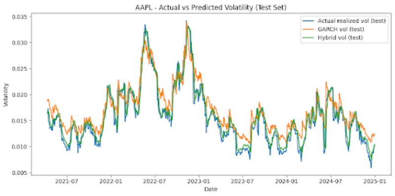
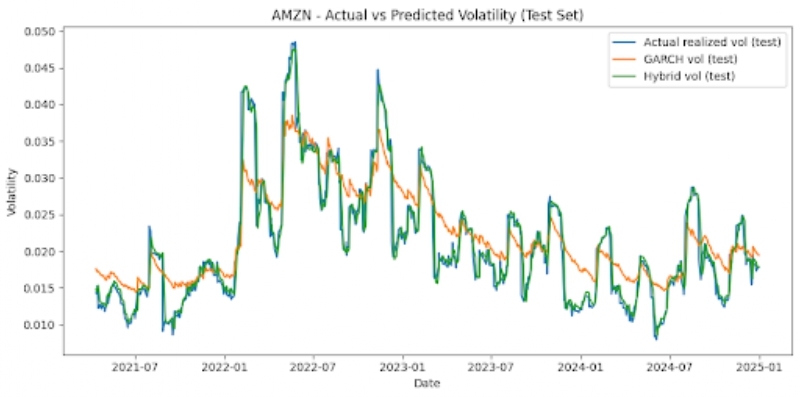
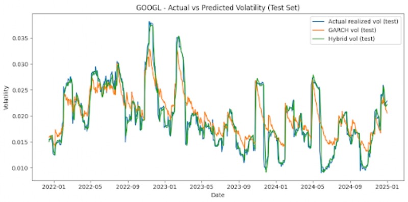
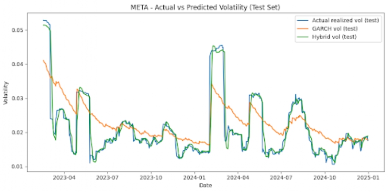
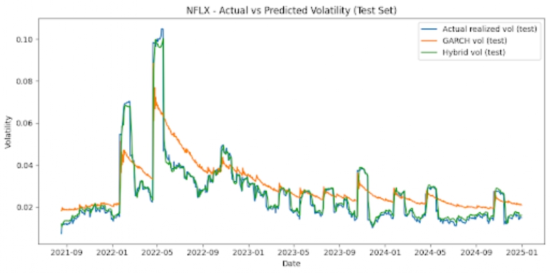
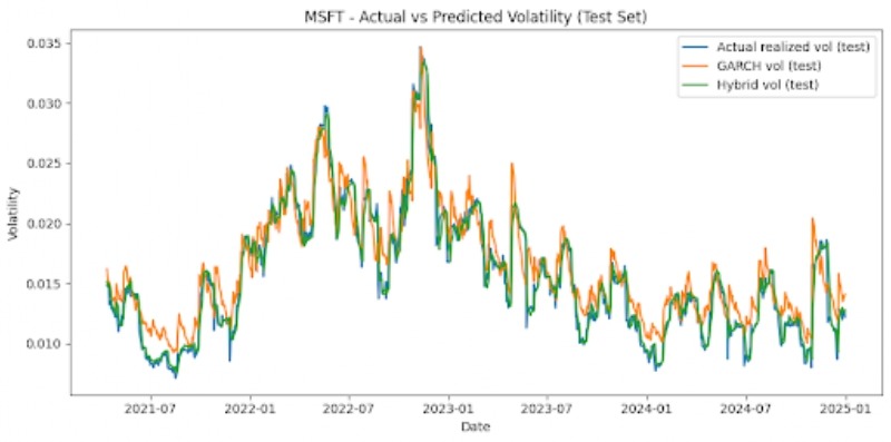
Noticeable patterns include that, for all six stocks, the hybrid model outperforms the GARCH model on the test set significantly. MSE is reduced by around 62-78% depending on the stock that is looked at. For instance, AAPL stock displays a GARCH MSE of 5.41 x 10^-6 and a hybrid MSE of 2.03 x 10^-6, signifying around a 62% reduction. The NFLX, a more volatile stock, shows a GARCH MSE of 9.02 x 10^-5 and a hybrid MSE of 2.07 x 10^-5, which is a reduction of around 77%. Additionally, we can also note that the LSTM and hybrid models have MSEs that are very similar. The hybrid model usually only offers very marginal improvements, and the optimal hybrid weight is effectively 1.0 for the LSTM forecast and 0 for the GARCH forecast. The hybrid and LSTM models both have very similar MSEs. The simple baselines unexpectedly offer strong predictions for stock market volatility, and are competitive with the LSTM and hybrid models for most instances. However, with less stable stocks like NFLX, the baseline and GARCH models perform comparatively worse than the hybrid and LSTM models. The GARCH model’s poor performance may be attributed to the fact that it is linear, has shorter memory, assumes constant parameters, lags volatility turning points, and isn’t designed for regime-switching markets. 

Rather than focusing solely on overall averages, MSE is computed individually for low-volatility and high-volatility test set areas. High volatility days are defined as days with a realized volatility that is above the 75th percentile of the test-set distribution, depending on the stock. Table 2 displays  MSEs that are regime-specific to  two representative tickers (to maintain brevity): AAPL and NFLX. This  offers a comparison of a stable stock versus a more volatile stock, and other stocks have patterns that are similar (figure 4). 

Stock	Model	High-volume MSE	Low-volume MSE
AAPL	GARCH	4.39 x 10-6	5.75 x 10-6
AAPL	LSTM	3.38 x 10-6	1.58 x 10-6
AAPL	hybrid	3.38 x 10-6	1.58 x 10-5
NFLX	GARCH	2.27 x 10-4	4.45 x 10-5
NFLX	LSTM	6.68 x 10-5	5.37 x 10-5
NFLX	hybrid	6.68 x 10-5	5.37 x 10-6

The patterns illustrate that the hybrid model outperforms GARCH on a consistent basis. In order to determine whether this improvement is statistically significant,  I applied the Diebold-Mariano test with squared error loss to the test-set forecasts for each stock. Across all of the stocks, the DM comparison for Hybrid vs GARCH appears to be a statistic that is positive and large. P values are also essentially 0. For example, the DM was around 15.7 for AAPL, 16.1 for AMZN, around 9.5 for META, 10.5 for GOOGL, 9.3 for NFLX, and 13.1 for MSFT. All of them had p values that were reported as 0.0 in double-precision output. This provides statistical evidence that the hybrid model is more accurate than the GARCH models. 

Beyond evaluation of model performance, this study offers new insights that previously have not been addressed in volatility forecasting research. This work offers a more concrete assessment of model behavior by comparing two baseline models, GARCH, LSTM, and a hybrid GARCH-LSTM using optimized weightage, for stocks that have high market capitalizations, utilizing over 20 years of historical stock data. Accuracy by regime is also quantified by this study, as it looks at model performance across periods that encompass high volatility and low volatility. The paper also includes statistical significance to prove that differences in model performance aren’t related to chance, and that there is a causal relationship between model type and prediction accuracy. This research also demonstrates that, if applied correctly, deep learning models have the potential to outperform classical econometric models. The aspect of optimal weightage shows that volatility dynamics change across stock and market conditions.      

Conclusion

Overall, the main purpose of this research was to compare the efficiencies of the GARCH model, the LSTM model, and a hybrid model dynamically weighting the results of both. Volatility is a key component of financial decision making, and having more accurate predictors can make it much easier for businesses and individuals to pinpoint critical and advantageous times to invest. Six stocks with large capitalizations were trained on realized volatility, or the 20-day rolling standard deviation of log returns, with a time/validation/test split of 70/15/15 including data spanning from earliest available date to the end of 2024.

The research offers several conclusions. The first is that traditional baseline models perform competitively with GARCH, LSTM, and the hybrid model, offering accurate volatility predictors, especially for stocks that are more stable. It was also found that while there is only a very marginal improvement between the LSTM and the hybrid model. For many stocks the optimal weight is close to 1.0, which indicates that the LSTM model is sufficient for predictivity. For other stocks, very minute GARCH predictions can offer small forecast stabilizations. The hybrid model periodically benefits from the GARCH model’s smoothness. 

A few limitations of the code are that different window lengths may produce slightly different results, since realized volatility only approximates actual volatility. While choosing 20 days is standard, there is a possibility that it could smooth out volatility patterns. Additionally, while diagnostics are included in the GARCH model, there may be occasional violations of white-noise assumption. This does not invalidate the model, since these violations are normal, but other volatility structures may be able to recognize additional dynamics. The hyperparameter tuning was also limited to a smaller grid to maintain reasonable computation, but more accurate model performance could occur with a larger grid search.  

Future research could incorporate a more expansive stock dataset, with other companies that have high market capitalization, in order to glean more accurate and extensive data. It could also include stock data that spans longer time periods. Additionally, models other than GARCH that have more predictive accuracy for these stocks can be tested with the LSTM model to determine whether a hybrid model can offer closer predictions. Additionally, LSTM could include features like macroeconomic variables, or sentiment indicators to learn more about stock market patterns from sources outside of the raw data. Data collected could also lead to more precise predictions by being based on smaller time windows; rather than analyzing daily stock data, data in 5 minute or 1 minute windows can be looked at. Concerning the creation of the hybrid model, another reasonable approach could be Markov-switching of the LSTM or GARCH models, leading to more accurate predictions that can better analyze changes between volatility regimes explicitly. 

Acknowledgements

I would like to thank Johnathan Delgadillo Lorenzo for guiding my efforts to build both the model and research, significantly assisting with my approach, and assisting with this paper.

References

1. E. F. Fama, K. R. French. Common risk factors in the returns on stocks and bonds. Journal of Financial Economics. Vol. 33, pg. 3–56, 1993, https://doi.org/10.1016/0304-405X(93)90023-5. [↩]
2. S. Gao, Z. Zhang, Y. Wang, Y. Zhang. Forecasting stock market volatility: The sum of the parts is more than the whole. Finance Research Letters. Vol. 55, pg. 103849, 2023, https://doi.org/10.1016/j.frl.2023.103849. [↩]
3. A. H. Munnell, M. S. Rutledge. The effects of the Great Recession on the retirement security of older workers. Annals of the American Academy of Political and Social Science. Vol. 650, pg. 124–142, 2013, https://doi.org/10.1177/0002716213499535. [↩]
4. R. Bhowmik, S. Wang. Stock market volatility and return analysis: A systematic literature review. Entropy. Vol. 22, pg. 522, 2020, https://doi.org/10.3390/e22050522. [↩]
5. E. Dávila, C. Parlatore. Volatility and informativeness. Journal of Financial Economics. Vol. 147, pg. 550–572, 2023, https://doi.org/10.1016/j.jfineco.2022.12.005. [↩]
6. J. Mansilla-Lopez, D. Mauricio, A. Narváez. Factors, forecasts, and simulations of volatility in the stock market using machine learning. Journal of Risk and Financial Management. Vol. 18, pg. 227, 2025, https://doi.org/10.3390/jrfm18050227. [↩]
7. R. F. Engle. Stock volatility and the crash of ’87. Journal of Empirical Finance. Vol. 6, pg. 341–344, 1999, https://doi.org/10.1093/rfs/3.1.77. [↩] [↩] [↩]
8. F. A. Gers, J. Schmidhuber, F. Cummins. Learning to forget: Continual prediction with LSTM. Neural Computation. Vol. 12, pg. 2451–2471, 2000, https://doi.org/10.1162/089976600300015015 [↩]
9. D. Kobiela, D. Krefta, W. Król, P. Weichbroth. ARIMA vs LSTM on NASDAQ stock exchange data. Procedia Computer Science. Vol. 207, pg. 3836–3845, 2022, https://doi.org/10.1016/j.procs.2022.09.445. [↩] [↩] [↩]
10. C. Delimitrou, C. Kozyrakis. Quasar: Resource-efficient and QoS-aware cluster management. Proceedings of ASPLOS. pg. 127-144, 2014, https://doi.org/10.1145/2654822.2541941. [↩]
11. C. Rudin. Stop explaining black box machine learning models for high-stakes decisions and use interpretable models instead. Nature Machine Intelligence. Vol. 1, pg. 206–215, 2019, https://doi.org/10.1038/s42256-019-0048-x. [↩]
12. C. T. Brownlees, G. M. Gallo. Comparison of volatility measures: A risk management perspective. Journal of Financial Econometrics. Vol. 8, pg. 29–56, 2010, https://doi.org/10.1093/jjfinec/nbp009. [↩] [↩] [↩]
13. G. W. Schwert. Why does stock market volatility change over time? Journal of Finance. Vol. 44, pg. 1115–1153, 1989, https://doi.org/10.1111/j.1540-6261.1989.tb02647.x. [↩] [↩]
14. M. A. Lubis, S. Samsudin. Using the random forest method in predicting stock price movements. Journal of Dinda. Vol. 5, pg. 28–35, 2025, https://doi.org/10.20895/dinda.v5i1.1765. [↩]
15. E. Ghysels, P. Santa-Clara, R. I. Valkanov. Predicting volatility: Getting the most out of return data sampled at different frequencies. NBER Working Paper No. 10914, 2004. [↩] [↩] [↩]
16. D. Kuvshinov, K. Zimmermann. The big bang: Stock market capitalization in the long run. Journal of Financial Economics. Vol. 145, pg. 527–552, 2022, https://doi.org/10.1016/ j.jfineco.2021.09.008. [↩]
17. Yahoo Inc. Yahoo Finance API documentation. 2024. [↩]
18. F. Cismondi, A. S. Fialho, S. M. Vieira, S. R. Reti, J. M. C. Sousa, S. N. Finkelstein. Missing data in medical databases: Impute, delete, or classify? Artificial Intelligence in Medicine. Vol. 58, pg. 63–72, 2013, https://doi.org/10.1016/j.artmed.2013.01.003. [↩] [↩]
19. P. Fortune. Weekends can be rough: Revisiting the weekend effect in stock prices. New England Economic Review Working Paper. No. 98–6, 1998. [↩] [↩]
20. M. Zheng, H.-S. Song, J. Liang. Modeling the volatility of daily listed real estate returns during economic crises: Evidence from generalized autoregressive conditional heteroskedasticity models. Buildings. Vol. 14, pg. 182, 2024, https://doi.org/10.3390/buildings14010182. [↩]
21. F. Ali, P. Suri, T. Kaur, D. Bisht. Modelling time-varying volatility using GARCH models: Evidence from the Indian stock market. F1000Research. Vol. 11, pg. 1098, 2022, https://doi.org/10.12688/f1000research.124998.2. [↩] [↩]
22. L. B. V. de Amorim, G. D. C. Cavalcanti, R. M. O. Cruz. The choice of scaling technique matters for classification performance. Applied Soft Computing. Vol. 133, pg. 109924, 2023. https://doi.org/10.1016/j.asoc.2022.109924. [↩]
23. T. G. Dietterich. Ensemble methods in machine learning. Multiple Classifier Systems, pg. 1–15, 2000, https://doi.org/10.1007/3-540-45014-9_1 [↩]
24. T. G. Dietterich. Ensemble methods in machine learning. Multiple Classifier Systems, pg. 1–15, 2000, https://doi.org/10.1007/3-540-45014-9_1. [↩]
25. M. E. Thomson, A. C. Pollock, D. Önkal, M. S. Gönül. Combining forecasts: Performance and coherence. International Journal of Forecasting. Vol. 35, pg. 474–484, 2019, https://doi.org/10.1016/j.ijforecast.2018.10.006. [↩] [↩]
26. G. Van Houdt, C. Mosquera, G. Nápoles. A review on the long short-term memory model. Artificial Intelligence Review. Vol. 53, pg. 5929–5955, 2020, https://doi.org/10.1007/s10462-020-09838-1. [↩] [↩]
27. P. C. Tetlock. Giving content to investor sentiment: The role of media. Journal of Finance. Vol. 62, pg. 1139–1168, 2007, https://doi.org/10.1111/j.1540-6261.2007.01232.x. [↩]
28. T. Bollerslev. Generalized autoregressive conditional heteroskedasticity. Journal of Econometrics. Vol. 234 (Supplement), pg. 25–37, 2023, https://doi.org/10.1016/j.jeconom.2023.02.001. [↩]
29. P. Mansfield. GARCH in question and as a benchmark. International Review of Financial Analysis. Vol. 8, pg. 1–20, 1999, https://doi.org/10.1016/S1057-5219(99)00002-2. [↩]
30. M. Escobar-Anel, L. Stentoft, X. Ye. The benefits of returns and options in the estimation of GARCH models: A Heston–Nandi GARCH insight. Econometrics and Statistics. Vol. 36, pg. 1–18, 2025, https://doi.org/10.1016/j.ecosta.2022.12.001. [↩]
31. F. A. Gers, J. Schmidhuber, F. Cummins. Learning to forget: Continual prediction with LSTM. Neural Computation. Vol. 12, pg. 2451–2471, 2000, https://doi.org/10.1162/089976600300015015. [↩] [↩] [↩] [↩] [↩] [↩]
32. Y. Zhang, T. Zhang, J. Hu. Forecasting stock market volatility using CNN-BiLSTM-attention model with mixed-frequency data. Mathematics. Vol. 13, pg. 1889, 2025, https://doi.org/10.3390/math13111889. [↩]
33. H. Y. Kim, C. H. Won. Forecasting the volatility of stock price index: A hybrid model integrating LSTM with multiple GARCH-type models. Expert Systems with Applications. Vol. 103, pg. 25–37, 2018, https://doi.org/10.3390/math13111889 [↩]
34. R. Alfaro, A. Inzunza. Modeling S&P500 returns with GARCH models. Latin American Journal of Central Banking. Vol. 4, pg. 100096, 2023, https://doi.org/10.1016/j.latcb.2023.100096. [↩]
35. B. Williams. Thesis. Department of Mathematics, University of California, Berkeley, 2011. [↩]
36. L. A. Gil-Alana, J. Infante, M. A. Martín-Valmayor. Persistence and long-run co-movements across stock market prices. The Quarterly Review of Economics and Finance. Vol. 89, pg. 347–357, 2023, https://doi.org/10.1016/j.qref.2022.10.001. [↩]
37. B. Gülmez. Stock price prediction with optimized deep LSTM network with artificial rabbits optimization algorithm. Expert Systems with Applications. Vol. 227, pg. 120346, 2023, https://doi.org/10.1016/j.eswa.2023.120346. [↩]
38. L. B. V. de Amorim, G. D. C. Cavalcanti, R. M. O. Cruz. The choice of scaling technique matters for classification performance. Applied Soft Computing. Vol. 133, pg. 109924, 2023. https://doi.org/10.1016/j.asoc.2022.109924. [↩]