Prometheus: A Recursively Self-Improving NAS System

Abstract

Neural Architecture Search (NAS) automates the process of neural network design, enabling the discovery of architectures that can surpass those manually constructed by human experts. For NAS systems involving a controller (often trained with reinforcement learning (RL)), one limitation is the intelligence of the controller. We introduce Prometheus to address this barrier. Project Prometheus is a series of NAS systems that utilize network morphism techniques, which allow edits to a neural network to be applied during training with minimal drop in performance, to edit both a convolutional neural network trained on image recognition tasks and also itself. The self-editing allows it to increase its own processing capacity to achieve better rewards from the RL system. Prometheus is currently in a proof- of-concept stage and has several limitations. One notable constraint is that the timing of its self-edits is governed by a human-defined heuristic, which restricts the system’s autonomy. Nevertheless, despite these early-stage limitations, the final system still achieves very competitive performance on the Canadian Institute For Advanced Research 10-class image dataset (CIFAR-10), achieving a mean accuracy of 95.47%±0.60%. It also performs competitively on the Street View House Numbers dataset (SVHN), the Fashion Modified National Institute of Standards and Technology dataset (Fashion-MNIST), and the CIFAR-100 dataset, with mean accuracies of 97.09%±0.15%, 95.57%±0.20%, and 73.26%±0.81% respectively.

Keywords: Neural Architecture Search, Reinforcement Learning, Self-Improving Systems, Artificial Intelligence, Deep Learning.

1. Introduction

Artificial Intelligence and machine learning have evolved exponentially in recent years. A particularly powerful branch of machine learning, called deep learning, uses models known as neural networks, which are computational systems loosely inspired by the structure of the human brain. The design of a neural network (the number of layers, the number of neurons per layer, etc.) is called its architecture. Using neural networks, deep learning has grown into an indispensable tool for humanity, allowing us to utilize patterns in data. However, designing an effective neural network architecture is often very intuition-based and time-consuming. Optimization often takes significant amounts of time and human effort. The subfield of neural architecture search (NAS) addresses this issue directly, as it seeks to automate the process of neural network architecture optimization.

There are many types of NAS systems, with the earliest forms being evolutionary algorithms, which use genetic algorithms to evolve network topologies. One notable work is that of Zoph and Le¹, which famously utilized over 500,000 GPU hours to find an optimal architecture, achieving a state-of-the-art accuracy of 96.35% on the Canadian Institute For Advanced Research 10-class image dataset (CIFAR-10). Subsequent works have striven to minimize the computational effort required to train NAS systems, like DARTS (Differentiable Architecture Search)²and ENAS (Efficient Neural Architecture Search)³,which rely on clever strategies like gradient-based search and weight sharing to lessen computation. More recent advances include extensible zero-cost proxies like Eproxy⁴,robust training-free NAS techniques⁵,and hardware-aware multi-objective differentiable NAS⁶.Beyond efficiency, several works tackle controller adaptability. MetaD2A⁷ demonstrates dataset-to-architecture transfer via meta-learning. Graph HyperNetworks⁸ generate weights directly from an architecture’s graph, allowing instant evaluation. Population Based Training⁹ shows that learners can improve themselves during training by mutating their hyperparameters. Learned optimizers¹⁰ replace hand-designed optimization rules with trainable neural controllers. Finally, NetAdapt¹¹ adapts networks mid-training to resource constraints using iterative pruning and morphism-based edits.

One notable strategy for adapting a network is network morphism.¹² Network morphism allows editing the overall architecture (macro-architecture) of a neural network during training without massive performance drops by initializing each new edit using its identity matrix, meaning that directly after performing the edit, the neural network is approximately identical to the original network, preventing performance drops.¹² This clever strategy was applied with reinforcement learning by Cai et al.¹³

Despite these clever strategies addressing the computational bottleneck of NAS, the reinforcement learning (RL) controllers within RL NAS studies are still human-designed and can require immense human trial and error to perfect. There does not yet exist a system that optimizes an RL controller along with the target network. To address this research gap, we propose Prometheus, a proof-of-concept NAS pipeline that uses network morphism and RL to optimize the architectures of both the network trained on the central task (the target neural network) and the RL controller. Even in its proof-of-concept stage, Prometheus still achieves competitive accuracies across all the datasets it was evaluated on, demonstrating the adaptability of the recursively self-editing system. This paper demonstrates the novel self-editing method first by going through 2 preliminary systems, then on to the full system of Prometheus. Details of Prometheus are illustrated in section 2. We presented experiments and results in section 3. Finally we discuss the system’s limitations and further implications in section 4.

2. Methods

Prometheus is a system designed to explore the following question: Can a model not only learn, but also learn how to improve itself? This idea of recursive self-improvement is a powerful conceptual precursor to artificial general intelligence (AGI). Prometheus attempts to embody that principle by developing a controller that evolves itself while evolving the neural networks it designs. The system supports self-pruning and growth in response to training signals such as stagnation and instability. All edits are function-preserving, achieved through Net2Net-style initialization.

Network Morphism

It is crucial to first define network morphism. Network morphism techniques allow the agent to modify the target network’s architecture without completely resetting its learned weights, accelerating the search process. The specific transformations implemented are:

• Net2Wider (widen): Following the Net2Wider operation from Chen et al.¹⁴, this action increases the width (number of output channels) of a convolutional layer. The weights for the new channels are initialized by replicating filters from the original layer, ensuring the new, wider layer can initially mimic the function of the old one.
• Net2Deeper (deepen): This operation, also from the original Net2Net¹⁴,increases network depth by inserting a new convolutional layer. The new layer is initialized to perform an identity mapping using a Dirac delta function for its weights. This allows the network to add the new layer without an initial drop in performance, giving it the capacity to learn a more complex function over time.
• Custom Thinning (thin): As the inverse of widening, we implemented a custom structured pruning operation. This action reduces a layer’s width by keeping the first k convolutional filters (where k is the new, smaller width) and discarding the rest. While this operation directly reduces model complexity and parameter count, it is a lossy transformation that alters the network’s function and relies on subsequent fine-tuning to recover performance.
• Custom Shallowing (shallow): To reverse the deepening process, we implemented a direct layer removal operation. This edit identifies a target convolutional layer and removes it, along with its subsequent normalization layer, from the network’s computational graph. This is our most aggressive complexity-reduction edit, as it fundamentally alters the network’s representational capacity.

2.1.     Preliminary Systems

System 1: LSTM Controller + Block-based Search + Basic Self-Edits

The first variant pairs a reinforcement learning agent (a long-short-term-memory (LSTM) controller) with pre-designed convolutional blocks (e.g., ResNet¹⁵, Inception¹⁶, SE-blocks¹⁷, Bottleneck Blocks¹⁸. Using network morphism, the controller could dynamically widen, deepen, or simplify the architecture during training. Crucially, this version introduces basic self-editing. The controller could widen or deepen its own LSTM architecture at fixed intervals, laying the groundwork for recursive improvement. Though the pre-designed blocks constrained its architectural expression, it was advantageous in its simplification of the task, especially when paired with a simple LSTM architecture.

System 2: GNN Controller + Fine-Grained Editing + Attention-Based Sampling

To address the inefficiency of block-level edits, System 2 replaces them with a granular, operation-level search. The controller, now a Graph Neural Network (GNN), represents the target convolutional neural network as a directed acyclic graph (DAG) and chooses from fine-grained edits like inserting individual 2D convolutional layers or Rectified Linear Unit (ReLU) layers, resizing channels, or creating skip connections. The controller self-edits using a new suite of GNN transformations, guided by attention mechanisms to focus search in promising regions. This expanded search space gives this system the expressive advantage, but it is harder to master this search space, which is why the RL controller was upgraded to a more complex GNN.

2.2. System 3

Search Space

System 3, our last iteration, returned to block-level editing (though more basic) while retaining the flexible, graph- based representation pioneered in System 2. The design objective was maximum stability with near-autonomous operation, so the GNN-driven reinforcement-learning controller remains at the core, yet both its action space and the environment’s feedback signals have been substantially enriched. At the architectural level, every permissible edit is a function-preserving block transformation. The following are the possible edits:

• Add Convolutional Block: Appends a Conv2d → 2d batch normalization → ReLU trio at a stage’s end. The Conv2d is identity-initialized, and 2d batch normalization starts with 𝛾 = 1.0, 𝛽 = 0.0, guaranteeing no immediate change in output (Net2Deeper style). After the block is appended using Net2DeeperNet, the agent chooses a channel multiplier to set the block’s width, which is applied using Net2WiderNet.
• Add Linear Block: Deepens the classifier by inserting a Linear → 1d batch normalization → ReLU right before the final layer. The new Linear layer is initialized as an identity matrix, again ensuring a function-preserving transformation. Once again, the agent is able to choose a width that is applied using Net2WiderNet.
  • Resize Layer: Selects any Conv2d or Linear node and scales its output dimension by a chosen factor. A learned attention head first pinpoints the most promising layer, then picks the resize factor.
  • Add Skip Connection: Creates a shortcut between two nodes within the same stage, chosen via attention over all valid source–destination pairs. If channel counts differ, an identity 1 × 1 convolution is inserted automatically to keep the DAG valid.

Evidently, the block-based search space of system 1 is adapted to be much simpler.

Initial Network

The search process is initialized with a simple VGG-style CNN backbone¹⁹ configured for the CIFAR-10 dataset. This starting architecture consists of three sequential stages. Each stage features a core block of Conv2d → 2d batch normalization → ReLU, with channel dimensions increasing from 64 to 128 and finally to 256. The first two stages are each followed by a 2 × 2 max-pooling layer for spatial downsampling. The feature extractor is connected to a classifier head composed of an adaptive average pooling layer and a single linear layer that maps the final 256-dimensional feature vector to the 10 output classes. This well-defined initial state serves as the starting point for all subsequent architectural modifications by the RL agent. In addition, the initial network was trained for 50 epochs at the start. If it hadn’t been initially trained, the first reward for the RL agent would always be massive and unrepresentative of the edit, as initial improvement to a neural network is usually fast.

Adaptive Training

To ensure stability and efficiency, the training process for both the target network and the RL controller is highly adaptive. For the target CNN, the number of post-edit training epochs scales in proportion to the parameter-change ratio, granting larger, more disruptive edits extra time to converge. The number of epochs, , is calculated as:

(1)  

where , and , are the parameter counts before and after the edit. Post-edit training utilizes a CosineAnnealingLR scheduler over this adaptive number of epochs. To further improve model performance, we apply strong augmentations, including \texttt{RandomCrop}, \texttt{RandAugment}, \texttt{RandomErasing}, and dataset-specific augmentations like \texttt{AutoAugment} when applicable. To accelerate training, the target CNN is trained using mixed precision with \texttt{autocast} and a \texttt{GradScaler}, and its gradients are clipped after each backward pass to prevent exploding gradients.

The RL component was optimized with Advantage Actor-Critic (A2C). The controller’s parameters and the value function’s parameters are updated by minimizing a composite loss function , which is composed of a policy loss for the actor, a value loss for the critic, and an entropy bonus to encourage exploration:

(2)  

where is the advantage, which is treated as a constant when updating the policy. The policy loss, , updates the actor () to make actions that produced a positive surprise more likely. The value loss, , is a mean-squared error term that trains the critic () to produce more accurate value estimates. Finally, is the policy entropy, and , are loss coefficients. For our system, the entropy bonus was set to , and the controller’s gradients are clipped to a maximum norm of 5.0 before each update.

Safety Nets

Stability is protected by safety nets. After every edit, the system performs a single-batch dummy training cycle to detect any immediate gradient problems that could cause “Not a Number” (NaN) values or structural errors. We set a maximum of 10 edit attempts per iteration, where if 10 edits fail, the iteration is considered failed and skipped (with -2 penalty per failed attempt, -5 for failed iteration). AMP auto-disables after 3 consecutive NaN batches to maintain stability. A rollback is triggered if acc_𝑡+1 < acc_best − 𝛿_rollback, where 𝛿_rollback = 0.04. Whenever a major architectural modification inflates the parameter count, the target CNN automatically triggers a warm-up schedule. During this phase, newly added batch normalization layers are initially frozen and then unfrozen over five “warm-up” epochs via a special learning rate ramp, preventing their untrained statistics from destabilizing gradients. Before committing any edit, we clone the current Target CNN via a deep copy and apply the proposed edit on this clone to project the post-edit parameter count. If the projected count exceeds 30 million parameters, we reject the action without touching the live model. In the case that the target neural network bypasses the check and reaches past 30 million parameters, the model is automatically reverted, and the controller is given a -50 reward. Whenever an edit alters the output channel dimension of a layer, the system immediately inspects the subsequent layer. If a dimensional mismatch is detected, the input channels of the subsequent layer are automatically rebuilt to match the new output dimension of the edited layer.

RL Controller

The RL controller is a GNN, specifically a Graph Convolutional Network (GCN)²⁰ that ingests the network’s DAG. In this formulation, the target CNN is represented as a graph G_𝑡 = (V, E), where each node 𝑣_𝑖 ∈ V represents an operation with a feature vector 𝑥_𝑖 ∈ R⁷. The feature vector encodes operation type, normalized output channels, stage and operator indices, stride, a binary convolution flag, and spatial dimensions. The target network begins as a simple three-stage backbone, which is then modified by the search process. Each operation (Conv2D²¹, ReLU²², etc.) is treated as a node, with edges representing data flow.

On every forward pass, the GCN performs message passing, letting each node aggregate information from its neighbors through multiple layers; the resulting graph-level context feeds into policy heads that issue structurally informed actions, surpassing the sequential view of an LSTM.

The GCN encoder processes the graph of the target network, , to produce a matrix of numerical representations (node embeddings), denoted by . The formal relationship is:

(3)  

The resulting matrix is defined as belonging to the space . This notation specifies the matrix’s structure and content:

• R indicates that the entries of the matrix are real numbers.
  • |V| is the total number of nodes (layers or operations) in the target network’s graph. This determines the number of rows in the matrix.
  • 𝑑_h is the dimensionality of the embedding for each node (e.g., a 128-dimensional vector). This determines the number of columns.

To make a decision, the controller needs a single, high-level summary of the entire network. This is achieved by creating a “global graph embedding,” 𝑧_𝑔, via mean-pooling. This process simply averages all the individual node embeddings:

(4)  

Here, 𝑧_𝑖 represents the embedding vector for a single node 𝑖 (i.e., the 𝑖-th row of matrix 𝑍), and the formula calculates their mean to produce a single, dense vector 𝑧_𝑔 representing the entire graph.

RL Implementation

The RL agent was given the ability to prune itself in addition to growing itself, but only after certain triggers. We define an iteration as one complete propose–train–evaluate cycle. If the validation accuracy does not beat the best validation accuracy after 5 iterations, a self-edit chosen by the RL agent along with a reversion to the best model occurs. A five-step window creates a balance between efficiency and guaranteed performance. When a model fails 3 dummy forward passes in a row, a self-edit occurs. While these heuristics serve as good measures to facilitate self-editing in this project, it is a limitation to the freedom of the RL agent. Upon triggering, we revert the target CNN weights to the best checkpoint so far, apply the sampled grow/prune action from the controller, and then resume the outer search loop. Growth choices comprise deepening the GNN, widening its hidden layers, and deepening a head, while pruning counterparts are pruning the GNN, shrinking the hidden layers, and pruning a head. Pruning options were only enabled after the meta-agent’s parameter count exceeded 15,000. The agent can thus expand its GNN depth, widen hidden sizes, or deepen policy heads when facing a harder search problem, yet later shed surplus capacity for efficiency once the task simplifies.

A replay buffer is also implemented to increase the richness of the meta-agent’s learning of self-edits. The replay buffer (capacity 50, batch size 8) stores (state, action, reward) triples for self-edits of the controller. The reward function

𝑅_𝑖 at iteration 𝑖 is formulated as:

(5)  

where is the post-edit validation accuracy, and is the pre-edit validation accuracy.

Finally, the meta-agent’s own learning rate is adaptive. It decays as the target model’s accuracy rises, enabling broad exploration early on and fine-grained exploitation near convergence. The meta-agent’s learning rate, 𝑙𝑟_meta, is annealed based on the target accuracy acc:

(6)  

where and define the accuracy range for annealing.

Attention Mechanism

As the architecture grows, the count of possible edits explodes. The agent employs an attention mechanism built atop the GNN’s node embeddings:

• Candidate identification: Enumerate all valid targets for the current action (every Conv2D for resizing, every legal pair for a skip).
  • Scoring: Feed the embeddings of these candidates into specialized heads that output a raw score (logit) per candidate. For a set of candidate nodes C, a scoring head 𝑓_score computes a logit 𝑞_𝑖 for each candidate node 𝑣_𝑖 ∈ C based on its embedding 𝑧_𝑖:

(7)  

• Probability distribution: Convert logits to a categorical distribution (softmax). The probability of selecting node 𝑣_𝑖 is given by:

(8)  

• Informed sampling: Sample from this distribution rather than greedily picking the top score, maintaining a balance between exploitation and exploration.

This combination of DAG-aware representation and attention-guided sampling enables Prometheus to navigate the immense edit space efficiently.

2.3  Reproducibility and Ethical Considerations

The three systems were all run on Google Colab Notebooks, and the link to them is here: https://github.com/ PlushyWushy/Prometheus/tree/main. This study exclusively utilized publicly available and anonymized image datasets, avoiding concerns related to human subject privacy or data confidentiality. The research adheres to standard scientific practices for reproducibility and responsible innovation. All experiments were conducted using PyTorch version 2.8.0, Torchvision 0.23.0, and PyTorch Geometric 2.6.1, running on Python 3.12 with CUDA support enabled via the +cu126 build. The discrete action space for resizing layers consisted of the factors [0.25, 0.5, 0.75, 1.25, 1.5, 1.75]. Other hyperparameters included: batch size = 128, AdamW learning rate = 0.001, dropout rate = 0.2, gradient clipping max norm = 5.0, BN recalibration over 200 batches, warm-up LR ramp over 5 epochs when parameter ratio > 1.2, meta-agent entropy coefficient = 0.001, edit-type embedding dimension = 16, initial GNN hidden dimension = 32 with 2 layers (minimums: 16 hidden units, 1 layer), maximum MLP head depth = 8, meta-agent replay buffer capacity = 50 with batch size 8.

3. Experiments and Results

To evaluate the performance and design principles of Prometheus, we conducted a series of experiments. Our evaluation is structured to analyze the evolution of our design by comparing the performance of our system variants and position our final system within the landscape of existing NAS methods.

3.1. Experimental Setup

Datasets

All three systems were evaluated on the CIFAR-10 dataset²³, which is a standard benchmark for image recognition and serves as the primary dataset for our development and comparative analysis. It consists of 60,000 32×32 color images across 10 balanced object classes, with 50,000 images for training and 10,000 for testing.

System 3 was additionally evaluated on the Street View House Numbers (SVHN), Fashion Modified National Institute of Standards and Technology (Fashion-MNIST), and CIFAR-100 datasets. The SVHN corpus²⁴ contains cropped 32×32 color images of house-number digits (0–9) collected from Google Street View, with 73,257 training samples and 26,032 test samples in the train–val split.

Fashion-MNIST²⁵, a tougher version of the original MNIST dataset, features 70,000 28×28 grayscale images across ten clothing categories, divided into 60,000 training examples and 10,000 test examples.

The CIFAR-100 dataset is another standard benchmark for image recognition and serves as a more challenging dataset for our system. It is a 100-class version of the CIFAR-10 dataset.

Implementation Details

We ran all searches on a single NVIDIA L4 Tensor Core GPU. The specific hyperparameters for each system variant were kept distinct to reflect their unique designs. For System 1, the target CNN was trained using AdamW with a weight decay of 10⁻⁴. The LSTM controller used an Adam optimizer with a learning rate of 5 × 10^-4 and a discount factor (𝛾) of 0.99. The A2C loss function used an entropy coefficient (𝛽_𝑒) of 0.01. The search was run for 150 iterations, and the reported accuracy is the average over 10 runs. For System 2, the target CNN was trained with AdamW (weight decay 5 × 10^-4) and a Cosine Annealing learning rate schedule. The GNN controller used an Adam optimizer with a learning rate of 5 × 10^-4. The search was regularized with MixUp (𝛼 = 0.4). The search was run for 200 iterations, and the reported accuracy is the average over 10 runs. For System 3, each search was run for 150 iterations. The meta-agent’s learning rate was annealed from a base of 5 × 10^-4 down to a minimum of 10^-5. All tests involving System 3 were conducted 10 times on random seeds.

3.2  Comparison of System Variants

We present a comparison of the three system variants on CIFAR-10. System 3 significantly outperformed the first two systems, achieving a final accuracy of 95.47%±0.60% (n=10) on CIFAR-10, while systems 1 and 2 achieved only 82.91%±5.16% (n=10) and 90.57%±0.68% (n=10), respectively. The key differences in methodology and the resulting trade-offs between performance and model complexity are summarized in Table 1.

Attribute	System 1	System 2	System 3
Controller	LSTM	GNN	GNN
Search Space	Block-Based	Granular	Block-Based
Final Params (Avg.)	28.0 M	2.6 M	12.5 M
Search Time (GPU Hours)	12	9	23
CIFAR-10 Acc. (%)	82.91±5.16	90.57±0.68		95.47±0.60

While the granular search of System 2 produced compact models (2.6M parameters average), its performance was limited. Though flexible, it had to navigate a massive search space, leading to a much harder policy to learn. In contrast, System 1, with its complex pre-designed blocks, discovered massive parameter networks that were numerically unstable and ultimately underperformed. It was given a toolkit of powerful blocks, but the simple LSTM controller was unable to combine them effectively. However, by pairing an intelligent, adaptive GNN controller with a powerful, structured block-based action space, System 3 discovers significantly more efficient architectures than System 1 that achieves higher accuracy. This demonstrates that the combination of a smart agent and an effective action space is extremely important for navigating the trade-offs between model complexity and performance.

3.3  Analysis of Self-Editing Mechanism

To isolate the direct impact of the recursive self-modification component, we conducted an ablation study comparing our full Prometheus System 3 with a version where the controller’s self-editing capabilities were disabled. In this ablated version, the GNN-based controller maintained a fixed architecture throughout the entire search. The average accuracies on CIFAR-10 are presented in Table 2.

System Variant	Self-Editing	CIFAR-10 Acc. (%)
System 3 (Ablated)	Disabled	95.10±0.55
System 3 (Full)	Enabled	95.47±0.60

The ablation shows a 0.37% average gain when the controller’s self-editing capability is enabled. To determine if this improvement was statistically significant, we performed a paired two-sample t-test on the results from each seed. The analysis confirms that the performance gain from self-editing is statistically significant (p = 0.012) at an 𝛼 = 0.05 level. This provides strong evidence that allowing the controller to adapt its own architecture during the search leads to the discovery of superior final network architectures.

3.4  Analysis of Search Space

To analyze the effectiveness of the block-based search space, we conducted an ablation study, comparing the full System 3 with a variant using the granular search space from System 2. The results are summarized in Table 3.

System Variant	Search Space	CIFAR-10 Acc. (%)
System 3 (Ablated)	Granular	85.45±0.65
System 3 (Full)	Block-based	95.47±0.60

The 10.02% average difference between the granular and block-based search spaces demonstrates the power of a structured search space. When held to the same standards and procedures as the full System 3, the granular search space fails to perform as well.

3.5  Comparison with Other NAS Methods

CIFAR-10

Method	Top-1 Acc. (%)
MetaQNN26	93.08
NAS-RL1	96.35
PNAS27	96.60
ENAS3	97.11
EAS13	95.77
DeepSwarm28	88.69
RSPS29	84.07±3.61
SETN30	87.64±0.00
DrNAS31	94.36±0.00
PC-DARTS32	93.66±0.17
GDAS33	93.61±0.09
First Order Differentiable Architecture Search (Our Impl.)	92.88±0.46
Prometheus (System 3) (Average)	95.47±0.60
Prometheus (System 3) (Best of 10 runs)	96.58

On the CIFAR-10 benchmark, Prometheus achieves a top-1 accuracy of 95.47%±0.60% (Table 4). Our system is competitive with its closest architectural antecedent, EAS¹³ (95.77%), and outperforms several modern differentiable methods, including DrNAS.³¹ Compared to the implemented differentiable architecture search system, Prometheus outperforms it by an average of 2.59%. Prometheus, despite operating on a more controlled, block-like search space, achieved a higher accuracy than the more flexible differentiable NAS. It is evident that a more structured search space can help a search system advance and that freedom is not always beneficial. The search times were relatively comparable, with the differentiable NAS search and retraining time taking 16 hours on average, versus Prometheus’s 23-hour average.

While top-performing methods like ENAS³achieve higher raw accuracy, Prometheus demonstrates that recursive self-editing can yield strong results as well. The novelty of its self-editing system positions it as a successful proof-of- concept, even against established NAS systems.

Street View House Numbers (SVHN)

To evaluate Prometheus beyond CIFAR-10, we benchmarked on the SVHN dataset. Since the SVHN dataset is relatively large compared to CIFAR-10, the training process was segmented into 3 50-iteration sessions due to Google Colab’s 24-hour code execution time limit, with the target neural network and RL controller being saved across the sessions. The total 150 iterations took 49 GPU hours. Table 5 compares our agent against recent controller-based or differentiable NAS approaches that report SVHN numbers in the same training regime.

Method	Accuracy (%)
DrNAS31	96.30
RSPS29	96.17
SETN30	96.02
GDAS33	95.57
PC-DARTS32	95.40
EAS13	98.27
ResNet-11034	98.27
Prometheus (System 3)	97.09±0.15

Prometheus surpasses every NAS baseline except for EAS in Table 5, despite using a single self-editing controller and no manual dataset-specific tuning.

Fashion-MNIST

Table 6 situates Prometheus among several evolutionary and swarm-based baselines.

Method	Accuracy (%)
MO-ResNet35 (best)	95.91
DeepSwarm28 (best)	93.56
Christoforidis et al.36	93.25
ECToNAS37	87.20
Prometheus (System 3)	95.57±0.20

Prometheus outperforms all except MO-ResNet (Table 6). MO-ResNet likely outperforms Prometheus on Fashion- MNIST because its residual-centric bias and a training pipeline tuned for small, grayscale data line up perfectly with the task, whereas our broader search space did not perform as well.

CIFAR-100

Table 7 compares Prometheus to various established methods on this more challenging dataset.

Method	Accuracy (%)
DrNAS31	73.51±0.00
GDAS33	70.70±0.30
PC-DARTS32	66.64±2.34
SETN30	59.09±0.24
RSPS29	52.31±5.77
Prometheus (System 3)	73.26±0.81

As seen in Table 7, Prometheus’s accuracy remains competitive in the landscape of established efficient NAS methods. The results on a more complex dataset position Prometheus as a solid system, even as a proof-of-concept for its self-editing mechanism.

3.6  Meta-Agent Growth

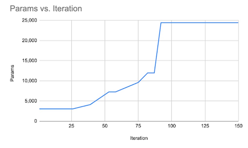
We analyzed the GNN controller’s architectural evolution over the course of a representative 150-iteration search run on CIFAR-10. The primary question was whether the controller would meaningfully alter its own structure in response to the search’s difficulty. Figure 1 illustrates the change in the controller’s total parameter count as the search progresses. The results provide strong empirical evidence of a dynamic and adaptive agent. The controller did not maintain a fixed architecture; instead, it grew significantly, starting with approximately 3,000 parameters and concluding with over 24,000, an 8-fold increase in complexity. In this run, there were no pruning operations conducted by the meta-agent in self-edits. Complexity was valued, as the increase in capacity of the model was often linked to a better target network performance.

4. Discussion

In this paper, we presented Prometheus, a NAS system grounded in the idea of recursive self-improvement. Through three successive variants, we showed that an RL-based controller can modify both a target network’s architecture and its own. Our final system, System 3, combines a self-editing GNN controller, a block-based action space, and heuristic-driven adaptation to achieve a competitive 95.47%±0.60% on CIFAR-10, performing well compared to its closest conceptual predecessor, EAS¹³ and supporting our approach as an effective search strategy.

Using triggers tied to stagnation and instability, the controller’s architecture is edited, intentionally trading short- term policy stability for longer-term capability. This behavior is enabled by function-preserving Net2Net edits that avoid catastrophic forgetting during self-modification. In theory, as the RL agent grows more capable, its edits to itself get better, causing it to grow even more capable, creating an ever-improving loop. We provide evidence that heuristic- triggered, function-preserving self-edits can improve search outcomes on small- to medium-scale vision benchmarks, offering a proof-of-concept for adaptive and autonomous NAS agents.

The progression through the three systems indicates that an extensively pre-designed block-level search (System 1) tends to inflate into inefficient, underperforming models. On the other hand, an overly granular, operation-level search (System 2) produces compact architectures but still struggles to find an optimal architecture. System 3 suggests a balanced path: a GNN controller manipulating basic blocks, guided by explicit complexity penalties and heuristic self-regulation. This is the system that ultimately outperformed the rest.

On the optimum triggers for self-editing, such as the stagnation window or rollback threshold, it is plausible that they would need to be adapted when scaling to more complex domains. A task like ImageNet, with its longer convergence times, might benefit from a different set of triggers to balance exploration and stability. An investigation into how these parameters scale with dataset complexity remains a crucial step toward creating a robust self-improving system.

4.1. Limitations

A key limitation of this study lies in its reliance on heuristic timing for self-editing. Specifically, the controller does not learn when to initiate edits; instead, it follows a set of predefined rules. This was an intentional design decision. As a proof-of-concept, our primary objective was to demonstrate that a controller could successfully modify its own architecture to better search performance, rather than to address the meta-learning challenge of optimizing the timing of such modifications. Employing a fixed trigger simplified the experimental setup and enabled us to more directly attribute performance improvements to the self-editing mechanism itself. Although a learned meta-policy would likely offer superior adaptability, our findings show that even a simple rule-based approach can produce measurable benefits, supporting the viability of heuristic self-regulation as a strategy for improving search quality.

Another limitation is type of evaluation datasets. The current evaluation focuses exclusively on image-based datasets. This leaves open the question of how well Prometheus would perform in other domains such as natural language processing, time series forecasting, or multimodal problems.

4.2. Future Work

Along with increasing the difficulty of the task at hand, future work could involve:

• Hierarchical RL: Training a high-level policy to decide when and how to self-edit, rewarding actions by the long-term gains of the lower-level (target-editing) policy.
  • Utility-Based Pruning: Inspired by synaptic pruning, replace instability heuristics with a mechanism that learns to remove the least useful components (e.g., neurons with minimal contribution), improving efficiency without blunt penalties.
  • Cross-domain evaluation: Extending Prometheus to non-vision domains such as text, time series, and audio, in order to validate its generality and adaptability.
  • Learned self-modification strategies: Replacing fixed heuristics with a learned meta-policy that enables the controller to autonomously decide when and how to alter its own architecture.

Together, these directions point toward the development of a truly autonomous NAS system, and one capable of learning not only architectures but also how to evolve itself over time.

References

1. Barret Zoph and Quoc V. Le. Neural architecture search with reinforcement learning. arXiv preprint arXiv:1611.01578, 2017. [↩] [↩]
2. Hanxiao Liu, Karen Simonyan, and Yiming Yang. Darts: Differentiable architecture search. arXiv preprint arXiv:1806.09055, 2018. [↩]
3. Hieu Pham, Melody Y. Guan, Barret Zoph, Quoc V. Le, and Jeff Dean. Efficient neural architecture search via parameter sharing. arXiv preprint arXiv:1802.03268, 2018. [↩] [↩] [↩]
4. Yuhong Li, Jiajie Li, Cong Hao, Pan Li, Jinjun Xiong, and Deming Chen. Extensible and efficient proxy for neural architecture search. arXiv preprint arXiv:2210.09459, 2023. [↩]
5. Zhenfeng He, Yao Shu, Zhongxiang Dai, and Bryan Kian Hsiang Low. Robustifying and boosting training-free neural architecture search. arXiv preprint arXiv:2403.07591, 2024. [↩]
6. Rhea Sanjay Sukthanker, Arber Zela, Benedikt Staffler, Samuel Dooley, Josif Grabocka, and Frank Hutter. Multi-objective differentiable neural architecture search. arXiv preprint arXiv:2402.18213, 2024. [↩]
7. Hayeon Lee, Eunyoung Hyung, and Sung Ju Hwang. Rapid neural architecture search by learning to generate graphs from datasets. arXiv preprint arXiv:2107.00860, 2021. [↩] [↩] [↩]
8. Chris Zhang, Mengye Ren, Raquel Urtasun, and Geoffrey E. Hinton. Graph hypernetworks for neural architecture search. arXiv preprint arXiv:1810.05749, 2018. [↩]
9. Max Jaderberg, Valentin Dalibard, Simon Osindero, Wojciech M. Czarnecki, Jeff Donahue, Ali Razavi, Oriol Vinyals, Tim Green, Iain Dunning, Karen Simonyan, Chrisantha Fernando, and Koray Kavukcuoglu. Population based training of neural networks. arXiv preprint arXiv:1711.09846, 2017. [↩]
10. Monika Wichrowska, Niru Maheswaranathan, Matthew W. Hoffman, and Jascha Sohl-Dickstein. Learned opti- mizers that scale and generalize. arXiv preprint arXiv:1703.04813, 2017. [↩]
11. Ting-Wu (T.-J.) Yang, Yu-Hsin (Y.-H.) Chen, and Vivienne Sze. Netadapt: Platform-aware neural network adaptation for mobile applications. arXiv preprint arXiv:1804.03230, 2018. [↩]
12. Tsui-Wei Wei, Chun-Pai Wang, and Yung-Yu Chen. Network morphism. arXiv preprint arXiv:1603.01670, 2016. [↩] [↩]
13. Han Cai, Tianyao Chen, Weinan Zhang, Yong Yu, and Jun Wang. Efficient architecture search by network transformation. arXiv preprint arXiv:1707.04873, 2018. [↩] [↩] [↩] [↩] [↩]
14. Tianqi Chen, Ian Goodfellow, and Jonathon Shlens. Net2net: Accelerating learning via knowledge transfer. arXiv preprint arXiv:1511.05641, 2016. [↩] [↩]
15. Kaiming He, Xiangyu Zhang, Shaoqing Ren, and Jian Sun. Deep residual learning for image recognition. arXiv preprint arXiv:1512.03385, 2015. [↩]
16. Christian Szegedy, Wei Liu, Yangqing Jia, Pierre Sermanet, Scott Reed, Dragomir Anguelov, Dumitru Erhan, Vincent Vanhoucke, and Andrew Rabinovich. Going deeper with convolutions. arXiv preprint arXiv:1409.4842, 2014. [↩]
17. Jie Hu, Li Shen, and Gang Sun. Squeeze-and-excitation networks. arXiv preprint arXiv:1709.01507, 2017. [↩]
18. Mark Sandler, Andrew Howard, Menglong Zhu, Andrey Zhmoginov, and Liang-Chieh Chen. Mobilenetv2: Inverted residuals and linear bottlenecks. arXiv preprint arXiv:1801.04381, 2018. [↩]
19. Karen Simonyan and Andrew Zisserman. Very deep convolutional networks for large-scale image recognition. arXiv preprint arXiv:1409.1556, 2014. [↩]
20. Thomas N. Kipf and Max Welling. Semi-supervised classification with graph convolutional networks. arXiv preprint arXiv:1609.02907, 2016. [↩]
21. Yann LeCun, Léon Bottou, Yoshua Bengio, and Patrick Haffner. Gradient-based learning applied to document recognition. Proceedings of the IEEE, 86(11):2278–2324, 1998. [↩]
22. Vinod Nair and Geoffrey E. Hinton. Rectified linear units improve restricted boltzmann machines. In Proceedings of the 27th International Conference on Machine Learning (ICML), pages 807–814, 2010. [↩]
23. Alex Krizhevsky and Geoffrey Hinton. Learning multiple layers of features from tiny images. Technical report, University of Toronto, 2009. [↩]
24. Yuval Netzer, Tao Wang, Adam Coates, Alessandro Bissacco, Bo Wu, and Andrew Y. Ng. Reading digits in natural images with unsupervised feature learning. In NIPS Workshop on Deep Learning and Unsupervised Feature Learning, 2011. [↩]
25. Han Xiao, Kashif Rasul, and Roland Vollgraf. Fashion-mnist: A novel image dataset for benchmarking machine learning algorithms. arXiv preprint arXiv:1708.07747, 2017. [↩]
26. Bowen Baker, Otkrist Gupta, Nikhil Naik, and Ramesh Raskar. Designing neural network architectures using reinforcement learning. arXiv preprint arXiv:1611.02167, 2016. [↩]
27. Chenxi Liu, Barret Zoph, Maxim Neumann, Jonathon Shlens, Wei Hua, Li-Jia Li, Li Fei-Fei, Alan Yuille, Jonathan Huang, and Kevin Murphy. Progressive neural architecture search. arXiv preprint arXiv:1712.00559, 2017. [↩]
28. Edvinas Byla and Wei Pang. Deepswarm: Optimising convolutional neural networks using swarm intelligence. arXiv preprint arXiv:1905.07350, 2019. [↩] [↩]
29. Lisha Li and Ameet Talwalkar. Random search and reproducibility for neural architecture search. arXiv preprint arXiv:1902.07638, 2020. [↩] [↩] [↩]
30. Xuanyi Dong and Yi Yang. One-shot neural architecture search via self-evaluated template network. arXiv preprint arXiv:1910.05733, 2019. [↩] [↩] [↩]
31. Xiangning Chen, Liang-Jie Xie, Jun Wu, and Qi Tian. Progressive differentiable architecture search: Bridging the depth gap between search and evaluation. arXiv preprint arXiv:2006.10355, 2020. [↩] [↩] [↩] [↩]
32. Yuhui Xu, Lingxi Xie, Xiaopeng Zhang, Xin Chen, Guo-Jun Qi, Qi Tian, and Hongkai Zhang. Pc-darts: Partial channel connections for memory-efficient differentiable architecture search. arXiv preprint arXiv:1907.05737, 2019. [↩] [↩] [↩]
33. Xuanyi Dong and Yi Yang. Searching for a robust neural architecture in four gpu hours. arXiv preprint arXiv:1910.04465, 2019. [↩] [↩] [↩]
34. reported by Lee et al. (Hayeon Lee, Eunyoung Hyung, and Sung Ju Hwang. Rapid neural architecture search by learning to generate graphs from datasets. arXiv preprint arXiv:2107.00860, 2021. [↩]
35. Shang Wang, Huanrong Tang, and Jianquan Ouyang. A neural architecture search method using auxiliary evaluation metrics based on resnet architecture. arXiv preprint arXiv:2505.01313, 2025. [↩]
36. Aristeidis Christoforidis, George Kyriakides, and Konstantinos Margaritis. A novel evolutionary algorithm for hierarchical neural architecture search. arXiv preprint arXiv:2107.08484, 2023. [↩]
37. Elisabeth J. Schiessler, Roland C. Aydin, and Christian J. Cyron. Ectonas: Evolutionary cross-topology neural architecture search. arXiv preprint arXiv:2403.05123, 2024. [↩]