Optimizing Drone-Based Crop Monitoring: An Analysis of the Shortest Path Problem

Abstract

The Shortest Path Problem is relevant across a wide range of domains, including search and rescue, logistics, and agricultural crop monitoring. This study compares the performances of three specific algorithms in solving the Shortest Path Problem for drone-based crop monitoring applications. A key constraint in this analysis requires the drone to return to its starting point, simulating real-world monitoring tasks. The three algorithms this study examines are the Traveling Salesman Problem (TSP) algorithm, Dijkstra’s algorithm, and A*. TSP employs a brute-force approach, Dijkstra’s algorithm relies on a cost function to determine the shortest path, and A* adds on to Dijkstra’s method with heuristics. The performance of these algorithms are evaluated based on total path length and computational efficiency. Each algorithm was tested multiple times on datasets containing three, five, ten, or eleven randomly generated points of interest to reduce the effects of errors or outliers. In this study, TSP achieved the highest accuracy, producing routes on average 6.3% shorter than those generated by Dijkstra’s and A*, with an average total path length of 284.6 units for 11 points. However, it suffered from exponential growth in computation time, reaching an average of 10.9 seconds at the same dataset size. In contrast, Dijkstra’s and A* algorithms offered significantly faster performance—5.1×10⁻³ and 1.1×10⁻² seconds respectively for 11 nodes—but produced longer paths. Dijkstra’s algorithm demonstrated greater computational efficiency than A*, outperforming it by an average of 3.45×10⁻³ seconds. These findings imply that, although A* is traditionally considered superior to Dijkstra’s algorithm, the unique constraint in this study—requiring the drone to return to its starting position—causes Dijkstra’s to significantly outperform A* by approximately an order of magnitude in computation time. This scenario of returning to the starting position is more representative of real-world conditions, where drones must return to a base station for charging and maintenance. These findings have practical implications for agriculture and drone-based surveillance, indicating that TSP is ideal for small-scale scenarios where accuracy is critical, whereas Dijkstra’s algorithm is better suited for larger-scale operations where computational speed is a priority.

Keywords: Pathfinding, Cost functions, Shortest Path Problem, Crop Monitoring, Algorithms, Agriculture

Introduction

In today’s rapidly evolving technological landscape, pathfinding algorithms are employed across a wide spectrum of disciplines including package delivery, wildfire suppression, and agricultural crop monitoring.

Our previous work at NASA¹ involved using drones with pathfinding capabilities and convolutional neural networks to detect disease in plants. This experience provided foundational insight into agricultural drone operations, particularly in generating efficient flight paths to investigate specific points of interest. In our XPRIZE Wildfire team, we implemented a pathfinding algorithm for multiple drones to navigate and suppress wildfires. Building upon this algorithm, we compared our new approach against the Rapidly Exploring Random Tree (RRT) algorithm for navigating complex wildfire environments. These efforts emphasize the growing need for efficient pathfinding algorithms to meet the demands of autonomous drone capabilities.

At the core of this need lies the Shortest Path Problem². This problem focuses on finding the optimal path between a starting node, a set of points to visit, and the end destination. The problem is represented by a 2D graph, with nodes and edges that represent the distances between them. These distances are what is used to determine the path that minimizes the total travel cost the most. In this study’s situation, the nodes represent points of interest that the farmer needs to investigate using a monitoring drone. This paper aims to evaluate which of three commonly used Shortest Path Problem algorithms is most effective for real-world drone-based crop monitoring. This study introduces a unique constraint not typically addressed: requiring the drone to return to its starting position, simulating actual operational needs like recharging or maintenance.

The Traveling Salesman Problem³ (TSP) aims to find the shortest route for a “salesman”—in this case a drone—to visit each city on a list once before returning to the starting point. This goal is accomplished by evaluating every possible permutation of the routes. However, initial testing revealed that TSP experienced significantly high computation times. In fact, when graphing results in bar charts, the execution times for Dijkstra’s and A* algorithms were so low that they appeared negligible next to TSP. As a result, a pruning function was implemented in the TSP algorithm to eliminate any permutations once the path exceeded a predefined upper bound. This limit was determined by finding the average distance between nodes, multiplying that value by the number of connections, and finally scaling it with an adjustable constant for flexibility. This modification drastically improved TSP’s computation time and resolved the aforementioned issues. Dijkstra’s algorithm⁴, known as a greedy algorithm, keeps a list of unvisited nodes. Beginning at the start point, the algorithm iteratively chooses the node with the smallest tentative cost (distance). The algorithm then visits all neighbors of that node and updates their tentative costs if a shorter path is found. This process is continued until it arrives at the destination. The A* algorithm⁵ approaches the Shortest Path Problem by considering both the cost to reach a node and the heuristic estimate of the remaining distance to the destination. A* selects the node with the lowest combined cost, continuing this process until the destination is reached.

Drone-based crop monitoring requires solving the Shortest Path Problem to efficiently visit multiple points of interest—such as crop fields—and return to a base station. This paper evaluates the performance of three prominent pathfinding algorithms—Traveling Salesman Problem (TSP), Dijkstra’s, and A*—by comparing their computation time and total path length under identical conditions. Each algorithm is tested on the same set of points with a fixed starting position. Unlike previous studies, this work introduces the constraint of requiring drones to return to the starting point, simulating real-world operational demands. The findings aim to help farmers optimize energy usage during remote drone monitoring by identifying which algorithm offers the best balance between accuracy and computational efficiency.

The comparison of the algorithms will be accomplished in four clear steps. The first step will be establishing the testing environment: this means defining the scale of the 2-dimensional map, generating the nodes, and selecting a start point. The second step will involve implementing The Traveling Salesman Problem, Dijkstra’s algorithms, and A* algorithm. The third step consists of data collecting and grading the speed and accuracy of the algorithms. The final step will be analyzing the data collected in step three to develop a conclusion. However, some limitations of this experimentation lies in the simplification of the problem. This analysis did not account for obstacles in between paths. In an ideal world obstacles can be ignored, but real world applications need to take into account obstacles that can hinder the movement of the monitoring drones.

Methods

The Traveling Salesman Problem⁶ (TSP) identifies the shortest path by evaluating all possible routes. Past papers and studies have applied TSP to optimize navigation through crop fields⁷, supplement truck-drone delivery systems using base stations⁸, and coordinate multi-drone package delivery with the assistance of trucks⁹. However, most of this prior work focuses on logistics-based applications or overlooks the importance of returning to a base station in agricultural contexts. This paper seeks to determine the use case of TSP in scenarios where a drone must return to the home base in an agricultural setting.

To improve computational efficiency, the implementation of the TSP algorithm includes a route termination feature: any route whose distance exceeds a calculated threshold is discarded. This upper limit is determined by multiplying the average distance between points by the total number of connections and an adjustable control factor. The number of connections is defined as the total number of points plus one, accounting for the return trip to the starting location. The control factor allows dynamic adjustment of the extent the algorithm prunes suboptimal paths. The application of this pruning function significantly reduced TSP’s computation time, making it more comparable to the other algorithms under evaluation. The equation used to calculate the limiting function, along with the corresponding pseudocode for the TSP implementation, is provided below.

   

Set starting and end point the same; Generate all (n-1)! permutations of routes; Calculate the distance for each permutation;    If cost > limit:      Terminate route; If total cost < current shortest route:       Set as new current shortest route; Return the route with the minimum cost;

Dijkstra’s algorithm¹⁰ determines the shortest path by selecting the node with the smallest tentative cost (distance) at each step.  It has been applied in past studies to optimize delivery routes for fresh agricultural products¹¹, improve the inefficiency of farm product collection and supply systems, and enable drone-based supply delivery to hard-to-reach areas¹². However, similar to the Traveling Salesman Problem, many of these studies either failed to create scenarios where the agent must return to the start position or apply the algorithm in an agricultural context.

It begins with initializing the distances between all nodes as infinity, except for the starting node, which is set at zero. The algorithm then visits the selected node, examines its neighbors, and updates their tentative distances if a shorter path is found. Once a node has been processed, it is marked as visited and is no longer considered for any future calculations. The process continues until all nodes are visited and the algorithm returns to the starting node. The following lines are the pseudo code for Dijkstra’s algorithm.

Mark the start node with a current distance of 0; Set all other nodes to infinity; Set every node as “non-visited”; While still unvisited nodes:   Select closest unvisited node; For each neighbor of current node:      Calculate tentative distance; Update neighbor’s distance if shorter; Mark current node as visited; Return route;

The A* algorithm¹³ finds the shortest path by combining two key factors: the actual cost from the start node to the current node, denoted as g(n), and the estimated cost from the current node to the goal, denoted as h(n). These are summed into the total cost function: f(n) = g(n) + h(n). In this study, the heuristic function h(n) is defined as the Euclidean distance, which effectively models the straight-line flight path a drone would follow in open, unobstructed agricultural environments.

The choice of heuristic is critical to A*’s performance. A well-chosen heuristic can significantly reduce computation time by guiding the algorithm toward the goal more efficiently, while a poor or overly generic heuristic may cause A* to behave similarly to Dijkstra’s algorithm—exploring unnecessary paths and increasing run time. In agricultural applications, where drones typically operate in flat, open fields, domain-specific heuristics like Euclidean distance are ideal. However, in more complex or obstacle-filled environments, other heuristics—such as Manhattan distance—may be necessary to ensure optimal performance.

Although the A* algorithm is used in robotics and AI applications, it has rarely been applied in agriculture or drone-based contexts. This study addresses that gap by evaluating the algorithm’s effectiveness in drone-based crop monitoring scenarios with the added constraint of returning to the starting position.

g(n) = cost from start node to the current node (n) h(n) = heuristic cost from current node (n) to end node f(n) = total cost of the node, where f(n) = g(n) + h(n)

The algorithm begins by placing the starting node in an open list and setting the values g(start) = 0 and f(start) = h(start). It selects the unvisited node with the lowest f(n) value as the current node and marks it as visited. If the current node is the goal, the shortest path has been found. If the goal is not reached, the algorithm evaluates each unvisited neighboring node and updates its g(n) and f(n) values if a cheaper path is found. The following lines are the pseudo code for A* algorithm.

Open list that holds all nodes; Closed node that tracks all nodes visited; While open_list != empty:   Choose node with lowest f(n) value;    Remove n from open_list and add to closed_list;    For each neighbor of n:      If neighbor is in closed_list:         Skip;       Calculate tentative g score;       If tentative g score < previous g score:         Update current_node;          g score of neighbor = tentative g score;          Calculate f score for neighbor;          Update heuristic estimate; If open_list empty && current_node != final_node:      Terminate, no path available;

The algorithms were performed on an Apple Mac Mini M1 with 8GB of memory, using PyCharm version 2024.1.4 64-bit evaluation copy. The methods for this experiment are as follows: initialization, algorithm execution, and data collection.

During the initialization phase, a set of points is generated using a random function, as shown in the code snippet below. A new random set of points is created for each trial to better reflect real-world conditions and ensure fair algorithm comparison. In real-world agricultural scenarios, the locations a drone must visit—such as crops flagged for potential disease or stress—are unlikely to follow a uniform or grid-like distribution. Instead, these points of interest are often scattered irregularly across the field. Additionally, randomizing the point sets for each trial reduces the likelihood that a specific node arrangement could unintentionally favor one algorithm over another. The generated points will be passed on as parameters to each algorithm. During the execution phase, all three algorithms will run, attempting to find the shortest route to visit all points in the quickest computation time possible.

points = pd.DataFrame({‘x’: np.random.rand(num_points) * 100, ‘y’: np.random. rand(num_points) * 100})

No obstacles were present on the map. This decision reflects common agricultural drone operations, where drones generally avoid obstacles by flying over them rather than navigating around them at ground level. Removing obstacles from the simulation focused the analysis solely on pathfinding efficiency, minimizing variables that could skew the comparison.

Finally, during the data collection phases, both computation time and total distance are calculated. The computation time is measured by recording the timestamp at the initiation of the algorithms as start_time. On completion, the start_time is subtracted from the current timestamp, code shown below.

computation_time = time.perf_counter() – start_time

The distance is calculated by iterating through the list containing the sequence of points visited by the algorithm and summing the distances between consecutive points. The distance between two points is calculated using the Pythagorean theorem, the formula shown below.

total_distance += calculate_distance(points.iloc[path[i]], points.iloc[path[i + 1]])

Our independent variable is the number of points the drone must visit. Experiments were conducted using 3, 5, 10, and 11 points, with each configuration run ten times to average the results and reduce the impact of outliers. The dependent variables were then measured as time and distance. The specific node counts were selected to create a holistic view of the algorithms’ performance across small to large-scale scenarios. Testing with only two nodes was excluded, as it did not yield meaningful insights. The analysis began with three points, then increased to five and ten to establish a consistent trend. Initially, a node count of 15 was set as the final count, but this proved impractical; beyond 11 nodes, the algorithm either required excessive computation time or failed to execute, making 11 the practical upper limit for this paper’s simulations.

Results

Algorithm	3 Nodes	5 Nodes	10 Nodes	11 Nodes
Traveling Salesman Problem	193.4 units	212.3 units	270.7 units	284.6 units
Dijkstra’s	193.4 units	220.6 units	293.1 units	318.0 units
A*	193.4 units	220.6 units	293.1 units	318.0 units

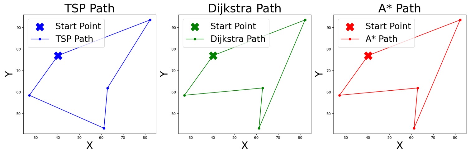
In terms of total distance traveled, Table Ⅰ demonstrates the Traveling Salesman Problem’s ability to return shorter routes compared to Dijkstra’s and A* algorithm. For three nodes, all algorithms yielded the same distance due to the limited routes possible. However, divergences in the paths traveled by the algorithms began as the number of nodes increased to five. Although many experiments still resulted in equal distances, TSP periodically found shorter routes, as reflected in the average values shown in Table I. The flight paths in Figure 1 further visualize these variations, highlighting how algorithmic behavior begins to diverge with the addition of more nodes. By the time the node count reached eleven, TSP consistently found shorter paths, averaging 284.6 units traveled, while Dijkstra’s and A* covered 318.0 units on average. The data highlights TSP’s accuracy compared to Dijkstra’s and A*, especially as the number of nodes increased. While Dijkstra’s and A* algorithms were accurate with smaller datasets, they had higher chances of choosing a nearest point that differed from the true shortest path as the dataset increased. On average, TSP found a route 6.3% shorter than Dijkstra’s and A*, making it the most accurate pathfinding algorithm of the three.

Algorithm	3 Nodes	5 Nodes	10 Nodes	11 Nodes
Traveling Salesman Problem	1.7e-5 sec	6e-5 sec	0.9 sec	10.9 sec
Dijkstra’s	4.9e-4 sec	8.1e-4 sec	3.3e-3 sec	5.1e-3 sec
A*	1.1e-3 sec	2.4e-3 sec	9e-3 sec	1.1e-2 sec

In terms of computation speed, the Traveling Salesman Problem demonstrated the fastest performance with fewer points. However, as Table II shows, TSP became inefficient as the number points increased as the computation time grew exponentially from 1.7 × 10⁻⁵ seconds with three nodes to 10.9 seconds with eleven nodes. This sharp increase in time exposes TSP’s permutational limitations. In contrast, Dijkstra’s algorithm had a more gradual increase in computational time, rising from 4.9 × 10⁻⁴ seconds for three nodes to 5.1 × 10⁻³ seconds for eleven nodes. The A* algorithm performed just below Dijkstra’s, taking 1.1 × 10⁻³ seconds for three nodes and 1.1 × 10⁻² seconds for eleven nodes. Similarly to Dijkstra’s algorithm, the A* algorithm starts out slower than TSP, but eventually executes faster as the number of nodes increases. Overall, the computation time data reinforces the notion that TSP excels with fewer points, while also demonstrating the capabilities of Dijkstra’s and A* algorithms as the number of points increases.

Discussion

In this study, by evaluating all possible permutations, the Traveling Salesman Problem yielded the most accurate results. For smaller datasets, TSP computed solutions faster than both Dijkstra and A* algorithms due to the reduced complexity and fewer permutations. However, TSP has major scalability drawbacks, making it impractical for large datasets. As the number of points increases, computation time grows exponentially, with eleven points taking approximately 10.9 seconds  on average. Despite the drawbacks, TSP remains accurate and can be applied in various scenarios.

Although the farmer’s 5-field monitoring case was not tested in the real world, results show that TSP yields routes 6.3% shorter than Dijkstra’s or A* across 11 nodes. This suggests that for small numbers of spatially dispersed points, where flight time is a major cost, TSP may be the most optimal method. While Dijkstra’s and A* algorithms would yield routes more quickly, TSP finds the shortest route. Since the crop fields are far apart, even small differences could be costly, making accuracy a higher priority than computation time. What appears to be 1 unit of distance on a map could represent a meter, a kilometer, or even a mile. Therefore, in scenarios where accuracy or optimal distance is critical, TSP is the superior algorithm.

Statistical analysis using Repeated Measures ANOVA, which compares the averages of multiple groups measured under different conditions, revealed a statistically significant difference in average total distances among the three algorithms (p < 0.05). Testing afterwards confirmed that TSP’s shorter path lengths were significantly better than those of Dijkstra’s and A*, especially at higher node counts. Similarly, an ANOVA on average computation time also found significant differences (p < 0.001), showing that TSP’s computation time increased sharply with more nodes, while Dijkstra’s and A* remained efficient. These results reinforce the conclusion that TSP is best suited for small-scale precision operations, but not for real-time or large-scale tasks.

In contrast, Dijkstra’s algorithm excels in computational efficiency, particularly when handling larger datasets. It outperformed both A* and TSP, especially when there are more than five points of interest. In this study, Dijkstra’s algorithm computed approximately 30% faster than A* algorithm on average. However, Dijkstra’s algorithm failed to consistently yield the most accurate path as the dataset grows. An increase in the number of points raises the probability of choosing the incorrect closest point. Despite this drawback, Dijkstra’s algorithm remains accurate in simple situations with smaller datasets. Additionally, its usefulness extends to situations involving large datasets or when minimizing computation time is more important than achieving the most accurate result. The measurements indicate that Dijkstra’s is approximately 30% faster than A* (5.1×10⁻³ s vs. 1.1×10⁻² s at 11 nodes). Thus, in scenarios demanding rapid response—such as diagnosing sporadic plant health issues—Dijkstra’s may be beneficial. However, this inference assumes node distributions and urgency levels similar to those in this study; further real-world validation is needed.

The main advantage of the A* algorithm is its balance of computational speed and accuracy. By using heuristics to guide its search, the A* algorithm generally outperforms Dijkstra’s in both computation time and accuracy—though in the trials conducted, this advantage was marginal due to the heuristic’s limited benefit when the start and final positions were the same. While A* took longer than Dijkstra’s in this experiment’s setup, its strength lies in cases where the end node differs, allowing the heuristic to prune the search space more effectively. While A* did not outperform Dijkstra’s in this study’s same start and end position, literature^14,15 shows A* excels in environments with asymmetric start and goal positions and where obstacles are present. Accordingly, incorporating heuristics in real-world missions with non-symmetrical navigation points could enhance performance—though this remains to be empirically evaluated.

In this study, the results indicate that the Traveling Salesman Problem (TSP) produced the most accurate paths, generating routes on average 6.3% shorter than Dijkstra’s and A*. However, it also experienced exponential growth in computation time, reaching 10.9 seconds for 11 nodes. Dijkstra’s algorithm achieved the best performance in terms of computational speed, averaging only 5.1×10⁻³ seconds, and proved to be about 30% faster than A* on average. While A* was expected to outperform Dijkstra’s due to its heuristic, its advantage was marginal in this study due to the start and end positions being the same. These findings achieve the study’s initial objectives of determining which of the three algorithms would be most effective in the real world for agriculture applications. While TSP is ideal for low-node, high-accuracy tasks, Dijkstra’s algorithm is better for large-scale, time-sensitive applications.  A* offers a compromise, particularly when destination nodes differ from starting positions.

Some limitations of this study include the limited range of trials and node counts tested. By only examining node counts of 3, 5, 10, and 11, it risks obscuring trends observable at intermediate values. Future research will involve expanded testing across a broader range of node counts to capture more accurate results. Another significant limitation is the absence of obstacles in the simulation environment. While this simplification aligns with certain agricultural use cases, it does not represent the complexity of real-world environments where obstacles—such as trees, irrigation systems, or uneven terrain—can greatly influence pathfinding performance. Future work should incorporate 3D terrain data and obstacle modeling to evaluate how each algorithm adapts in constrained navigation scenarios. Finally, we plan to integrate Convolutional Neural Networks and hyperspectral imaging to detect crop disease, combining those outputs with our pathfinding algorithms for real-time autonomous navigation. This integrated approach will help validate our initial hypothesis(8) and potentially offer a system for smart agricultural monitoring.

Acknowledgments

Our previous work at NASA involved developing a system for drones to analyze crops for disease using convolutional neural networks. We have also worked on our AMSE Wildfire team, sponsored by the XPRIZE foundation, specifically the drone’s ability to pathfind to fires. Additionally, we have competed in science fairs involving pathfinding algorithms and their applications to wildfire response.

References

1. Yotam Dubiner, S. Hahm, J. Low, A. Nguyen, P. Singh, and Y. Sung, “Plant Disease Detection: Exploring Applications in Hyperspectral Imaging and Machine Learning for Agriculture,” Nasa.gov, Aug. 2023. https://ntrs.nasa.gov/citations/20230013018 (accessed Sep. 21, 2024). [↩]
2. A. Schrijver, “On the History of the Shortest Path Problem,” 2012. [↩]
3. D. Applegate, R. Bixby, V. Chvátal, and W. Cook, “On the Solution of Traveling Salesman Problems,” Doc. Math. J. DMV Documenta Mathematica · Extra, vol. ICM, pp. 645–656, 1998. [↩]
4. K. Magzhan and H. Mat Jani, “A Review and Evaluations of Shortest Path Algorithms,” Int. J. Sci. Technol., Jun. 2013. [↩]
5. “Geometric A-Star Algorithm: An Improved A-Star Algorithm for AGV Path Planning in a Port Environment | IEEE Journals & Magazine | IEEE Xplore,” ieeexplore.ieee.org, 2021. https://ieeexplore.ieee.org/abstract/document/9391698 [↩]
6. N. Sathya and A. Muthukumaravel, “A Review of the Optimization Algorithms on Traveling Salesman Problem,” Indian Journal of Science and Technology, vol. 8, no. 29, Nov. 2015, doi: https://doi.org/10.17485/ijst/2015/v8i1/84652. [↩]
7. I. Ait, E. Kofman, and T. Pire, “A Travelling Salesman Problem Approach to Efficiently Navigate Crop Row Fields with a Car-Like Robot,” IEEE Latin America Transactions, vol. 21, no. 5, pp. 643–651, May 2023, doi: https://doi.org/10.1109/tla.2023.10130836. [↩]
8. S. Kim and I. Moon, “Traveling Salesman Problem With a Drone Station,” IEEE Transactions on Systems, Man, and Cybernetics: Systems, vol. 49, no. 1, pp. 42–52, Jan. 2019, doi: https://doi.org/10.1109/tsmc.2018.2867496. [↩]
9. Z. Luo, M. Poon, Z. Zhang, Z. Liu, and A. Lim, “The Multi-visit Traveling Salesman Problem with Multi-Drones,” Transportation Research Part C: Emerging Technologies, vol. 128, p. 103172, Jul. 2021, doi: https://doi.org/10.1016/j.trc.2021.103172. [↩]
10. M. H. Xu, Y. Q. Liu, Q. L. Huang, Y. X. Zhang, and G. F. Luan, “An improved Dijkstra’s shortest path algorithm for sparse network,” Applied Mathematics and Computation, vol. 185, no. 1, pp. 247–254, Feb. 2007, doi: https://doi.org/10.1016/j.amc.2006.06.094. [↩]
11. Y. Tan and D. Wu, “Research on Optimization of Distribution Routes for Fresh Agricultural Products Based on Dijkstra Algorithm,” Applied Mechanics and Materials, vol. 336–338, pp. 2500–2503, Jul. 2013, doi: https://doi.org/10.4028/www.scientific.net/amm.336-338.2500. [↩]
12. A. M. Deaconu, Razvan Udroiu, and Corina-Ştefania Nanau, “Algorithms for Delivery of Data by Drones in an Isolated Area Divided into Squares,” Sensors, vol. 21, no. 16, pp. 5472–5472, Aug. 2021, doi: https://doi.org/10.3390/s21165472. [↩]
13. M. R. Wayahdi, S. H. N. Ginting, and D. Syahputra, “Greedy, A-Star, and Dijkstra’s Algorithms in Finding Shortest Path,” International Journal of Advances in Data and Information Systems, vol. 2, no. 1, pp. 45–52, Feb. 2021, doi: https://doi.org/10.25008/ijadis.v2i1.1206. [↩]
14. W. Zhang, J. Li, W. Yu, P. Ding, J. Wang, and X. Zhang, “Algorithm for UAV path planning in high obstacle density environments: RFA-star,” Frontiers in Plant Science, vol. 15, Oct. 2024, doi: https://doi.org/10.3389/fpls.2024.1391628. [↩]
15. S. Chakraborty, D. Elangovan, P. L. Govindarajan, M. F. ELnaggar, M. M. Alrashed, and S. Kamel, “A Comprehensive Review of Path Planning for Agricultural Ground Robots,” Sustainability, vol. 14, no. 15, p. 9156, Jan. 2022, doi: https://doi.org/10.3390/su14159156. [↩]