
Abstract
The S&P 500 index which comprises 500 of the largest publicly traded companies in the United States (US) is widely recognized for its fluctuating behavior. Stock volatility is a measure of how much and how quickly a stock’s price (or a market index such as the S&P 500) moves up and down over time. Accurately forecasting the fluctuations in S&P 500 volatility is crucial for investors seeking to maximize returns and businesses that rely on such predictions for strategic financial planning and operations. Traditionally, this task is approached using sophisticated statistical models which often experience limited accuracy and inefficiency when capturing complex and nonlinear patterns in financial time series data. Advancements in machine learning have opened the door to developing Artificial Intelligence (AI) models that can predict stock volatility with improved accuracy and effectiveness. There has been limited research that utilizes machine learning to study the relationships between economic indicators and stock volatility; this area remains underexplored. This study employs a comparison of various forecasting models to identify the most accurate machine learning model for predicting S&P 500 volatility based on US economic indicators which were chosen because of their proven significance in representing macroeconomic conditions and their potential impact on S&P 500 volatility. More specifically, this research evaluated Neural Networks: Long Short-Term Memory (LSTM) (a type of Recurrent Neural Networks (RNN)) and Feedforward Neural Networks (FNN), traditional supervised machine learning models: Linear Regression, Lasso Regression, Decision Trees, and Random Forests, statistical models: Generalized Autoregressive Conditional Heteroscedasticity (GARCH) and AutoRegressive Integrated Moving Average (ARIMA), and baseline model: mean forecast method, where the statistical and baseline models were used to show whether the most accurate machine learning method provided higher accuracy. The predictive accuracy, measured by Root Mean Square Error (RMSE), of each model was assessed to identify the most effective one. The hypothesis states that LSTM would outperform the other models since it is the most suitable for problems related to time series data. The results confirm this as LSTM achieved the lowest RMSE, indicating its comparatively strong capability in predicting S&P 500 volatility using US economic indicators.
Introduction
Accurately and efficiently predicting S&P 500 volatility is essential for individuals and organizations seeking to minimize investment risks1‘2. Before the adoption of machine learning in finance, forecasting methods primarily relied on complex mathematical and statistical models including Generalized Autoregressive Conditional Heteroscedasticity (GARCH) and Autoregressive Conditional Heteroskedasticity (ARCH) models3. These approaches often lack accuracy and are computationally inefficient because they rely on past errors to estimate volatility and can struggle when data exhibits strong persistence in variability, a common characteristic of financial time series data4‘5‘6. Previous research has highlighted the superior accuracy of machine learning models7‘8. For instance, one study comparing Neural Networks and statistical models such as GARCH and Autoregressive Moving Average (ARMA)9 finds that statistical models are not only less accurate but also more complex and difficult to optimize compared to machine learning approaches10. Given the strong influence of economic conditions on stock market behavior, incorporating economic indicators into predictive models has become increasingly important11‘12. Therefore, the objective of this research is to determine the most accurate machine learning model for predicting S&P 500 volatility using US economic indicators.
Several recent studies have aimed to determine the most effective machine learning model for forecasting S&P 500 volatility and price movements, using either US economic indicators or technical indicators data13‘14‘15. One research finds that a hybrid Deep Convolutional Neural Network (DCNN) outperforms a standard Convolutional Neural Network (CNN) in this task13. Another analysis comparing Baseline Linear Regression, Feedforward Neural Networks (FNN), Decision Trees, and Random Forests concludes that Random Forest provides the highest predictive accuracy among the models tested14. Similarly, additional research evaluating models such as Logistic Regression, Linear Regression, Random Forest, Bagging Regression, Gradient Boosting Regression, Ridge Regression, and Lasso Regression also identifies Random Forest as the most effective15. Despite these contributions, there is still a lack of studies directly comparing Neural Networks, traditional supervised machine learning models, statistical models, and baseline models. This gap motivates the present study which compares Long-Short Term Memory (LSTM) (a type of Recurrent Neural Networks (RNN)), FNN, Linear Regression, Lasso Regression, Decision Trees, Random Forests, GARCH, AutoRegressive Integrated Moving Average (ARIMA) (a type of ARMA), and mean forecast model to identify the machine learning model that can most accurately predict stock volatility based on US economic indicators. The statistical and baseline models were employed to evaluate whether the most accurate machine learning method demonstrated higher accuracy compared to non-machine learning models. The predictive accuracy of each technique was assessed using Root Mean Square Error (RMSE), with the machine learning models’ prediction fit graphs serving as supplementary illustrations. The LSTM model is included in this comparison due to its strength in modeling sequential data, making it particularly well-suited for time series forecasting tasks such as stock volatility prediction16‘17.
Methodology
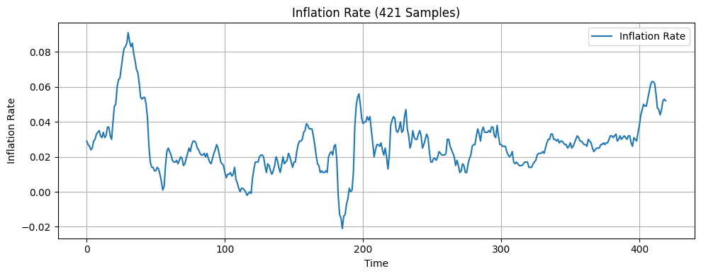
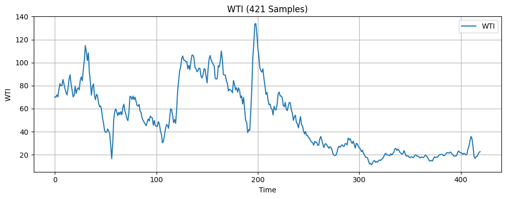
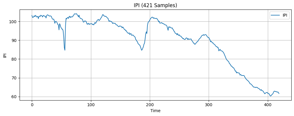
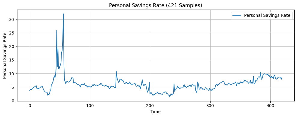
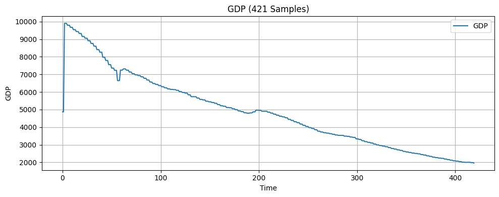
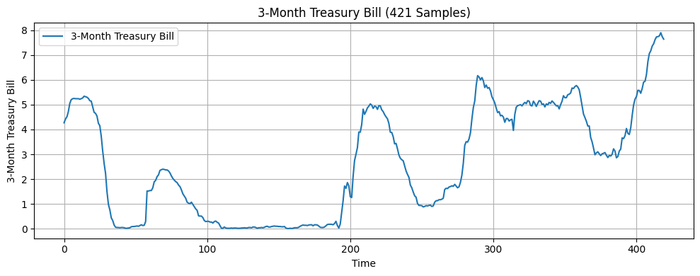
In this research, the input features include seven economic indicators: US monthly inflation rate18, US monthly unemployment rate19, US monthly West Texas Intermediate (WTI) crude oil price20, US monthly Industrial Production Index (IPI)21, US monthly personal saving rate (PSAVERT)22, US quarterly Gross Domestic Product (GDP)23, and US monthly 3-month Treasury Bills rate (TB3MS)24. These seven indicators were selected because they broadly represent the main drivers of economic activities, covering growth, inflation, employment, consumer behavior, financial markets, and monetary policy14‘25. Months are also one of the features since incorporating temporal information is considered good practice when working with time series data16. The target variable is the monthly volatility of the S&P 500 index, calculated as the standard deviation of its daily returns over each month26. The dataset consists of 421 samples, each containing the eight features above and the one target variable. A visualization of the economic indicators is presented in Figure 1.

The original dataset was split sequentially into three subsets: 64% for training, 16% for validation, and 20% for testing. Following this train-validation-test split, a look-back window was applied to each subset, transforming the data into overlapping sequences of fixed length where each input sample was composed of a sequence of consecutive observations of features, determined by the specified look-back window, and the next data point in the target series. This transformation enabled the model to capture the temporal dependencies within the economic indicators. After this preprocessing step, all three datasets were standardized using a scaling method before being fed into the machine learning models.
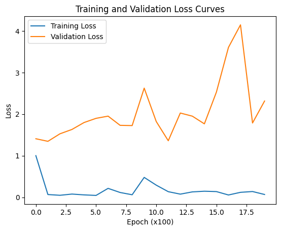
The first machine learning model evaluated in this study was LSTM27. It was trained, validated, and tested on training, validation, and test sets, respectively. During training, overfitting was observed. To mitigate this issue, hyperparameters—the look-back window, learning rate, batch size, number of layers, and dropout rate—were tuned, and subsequently, cross-validation and data augmentation which adds noise to the expanded datasets were utilized. In the search for an optimal setup, grid search was applied, and the combination yielding a validation loss curve with the steepest and most consistent downward trend was chosen. The best results were achieved by expanding the training set to 4000 samples with a sigma of 0.09, combined with a hyperparameter configuration consisting of a look-back window of 17, a batch size of 8, three layers, and a learning rate of 0.01. However, this setup only modestly reduced overfitting. In order to better assess the accuracy level of each machine learning model, both the original and augmented datasets were used for training and comparison.
Table 1 presents the hyperparameter ranges used in the LSTM grid search, while Table 2 details the data augmentation ranges used in the LSTM grid search.
| Look back window | Learning rate | Batch size | Number of layers | Dropout number |
|---|---|---|---|---|
| 11 – 20 | 0.01 – 0.1 | 8 – 16 | 1 – 3 | 0.2 – 0.4 |
| Number of training samples | Number of validation samples | Sigma value |
|---|---|---|
| 2000 – 64000 | No augmented validation set – 16000 | 0.09 – 0.2 |
Other than LSTM, FNN28‘29, Linear Regression30, Lasso Regression31, Decision Trees32‘33, Random Forest34‘35, GARCH3, and ARIMA36 were also employed. The last model utilized was the mean forecast model which was intended to show whether the LSTM model provided higher accuracy than the baseline method. Hyperparameter tuning was conducted for the Decision Tree model across max depth, min samples split, min samples leaf, and random state, and for the Random Forest model across max depth and random state. The Decision Tree model achieved the most accurate results using a max depth of 5, a min samples split of 10, a min samples leaf of 5, and a random state of 42. The Random Forest model obtained the most accurate results using a max depth of 2 and a random state of 0. Data augmentation was not applied to the GARCH, ARIMA, and mean forecast models since they don’t rely on artificially generated data in the same way as machine learning models do.
The predictive accuracy of each model was assessed using test RMSE, with the machine learning models’ prediction fit graphs serving as supplementary illustrations, and then compared across models to evaluate their relative effectiveness.
Results
After hyperparameter tuning, cross validation, and data augmentation, the signs of overfitting exhibited by the LSTM model were modestly mitigated by augmenting the training data to 4000 samples using a sigma of 0.09, with a batch size of 8, three layers, a learning rate of 0.01, and a look-back window of 17.
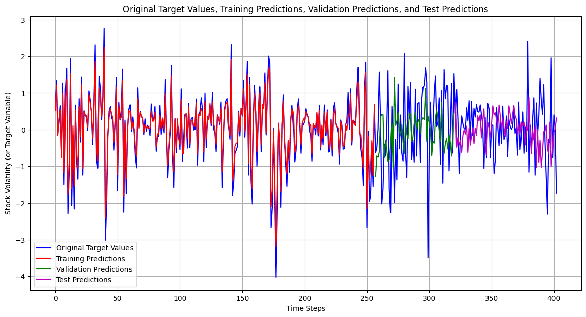
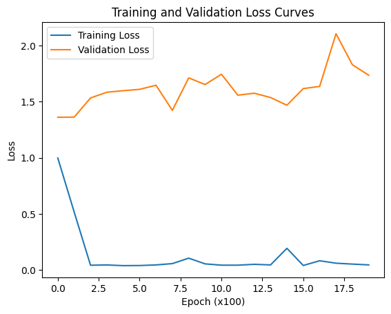
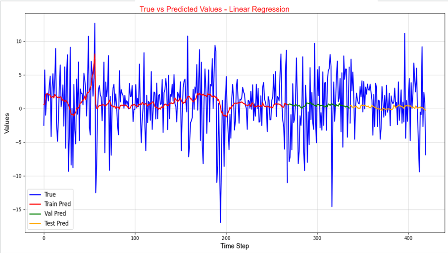
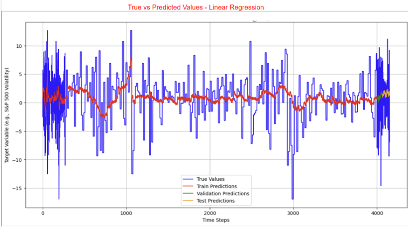
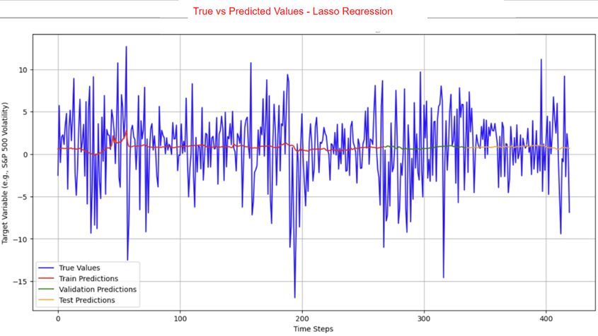
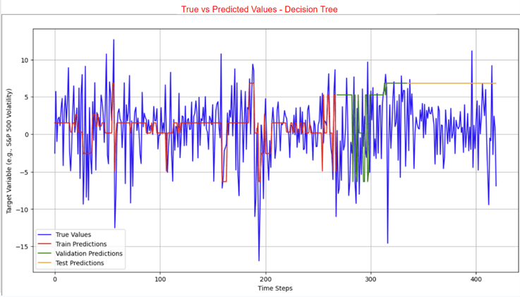
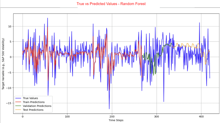
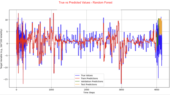
The LSTM, FNN, and traditional supervised machine learning models were trained on both the 421 samples and the 4000 training samples, whereas the statistical and mean forecast models were trained on the 421 samples only. Tables 3 and 4 present the RMSE and R² values for the LSTM model. Table 5 provides the RMSE of the FNN, the traditional supervised machine learning models, the statistical models, and the mean forecast approach. Table 6 summarizes a comparison of the test RMSE of all models in this research. Figures 2 and 3 show the prediction fit graphs and the train and validation loss curves for the LSTM model. Figure 4 illustrates the prediction fit graphs for the traditional supervised machine learning models. The prediction fit graphs of the FNN model are omitted, as they reduce to two straight lines without variation, underscoring that the FNN model underperformed relative to both the LSTM and the traditional supervised machine learning models.
| Train RMSE | Validation RMSE | Validation R² | Test RMSE | Test R² |
|---|---|---|---|---|
| 0.215 | 1.318 | -0.291 | 0.92 | -0.49 |
| Train RMSE | Validation RMSE | Validation R² | Test RMSE | Test R² |
|---|---|---|---|---|
| 0.259 | 1.521 | -0.647 | 1.059 | -0.893 |

Figure 3 | a): Original target values vs predicted target values for the LSTM model (4000 training samples). This graph displays the original target values (blue) compared to the training predictions (red), the validation predictions (green), and the test predictions (purple) across the entire period.
| Model | Train RMSE | Validation RMSE | Test RMSE |
|---|---|---|---|
| FNN (421 samples) | 4.000 | 5.000 | 5.000 |
| FNN (4000 training samples) | 4.000 | 5.000 | 5.000 |
| Linear Regression (421 samples) | 4.135 | 5.076 | 3.484 |
| Linear Regression (4000 training samples) | 4.076 | 5.087 | 3.453 |
| Lasso Regression (421 samples) | 4.238 | 5.117 | 7.002 |
| Lasso Regression (4000 training samples) | 4.196 | 5.122 | 4.086 |
| Decision Tree (421 samples) | 3.737 | 7.347 | 6.739 |
| Decision Tree (4000 training samples) | 3.527 | 6.578 | 8.981 |
| Random Forest (421 samples) | 2.409 | 5.385 | 3.369 |
| Random Forest (4000 training samples) | 2.084 | 6.495 | 3.433 |
| GARCH (421 samples) | 1.013 | 1.825 | 1.124 |
| ARIMA (421 samples) | 1.509 | 1.601 | 1.760 |
| Mean Forecast (421 samples) | 4.360 | 5.061 | 3.297 |


| Model Type | Model | Test RMSE From 421 Samples | Test RMSE From 4000 Training Samples |
|---|---|---|---|
| Neural Networks | LSTM | 0.920 | 1.059 |
| FNN | 5.000 | 5.000 | |
| Traditional Supervised Machine Learning Models | Linear Regression | 3.484 | 3.453 |
| Lasso Regression | 7.002 | 4.086 | |
| Decision Tree | 6.739 | 8.981 | |
| Random Forest | 3.369 | 3.433 | |
| Statistical Models | GARCH | 1.124 | N/A |
| ARIMA | 1.760 | N/A | |
| Baseline Model | Mean Forecast | 3.297 | N/A |
Discussion
Based on the test RMSE comparison of the LSTM, the FNN, the traditional supervised machine learning models, the GARCH model, the ARIMA model, and the mean forecast method, it can be concluded that the LSTM model consistently provides higher predictive accuracy than the others, regardless of the data augmentation, which supports the original hypothesis. With 421 samples, the FNN model achieved a test RMSE of 5.000 which is higher than the LSTM model’s test RMSE of 0.920. The LSTM model also outperforms the traditional supervised machine learning models whose test RMSE ranged from 3.369 to 7.002. Among the statistical models, the GARCH model recorded a test RMSE of 1.124, while the ARIMA model obtained 1.760, proving that the statistical models perform worse than the LSTM model. The LSTM model also proves to be more effective than the mean forecast model which achieved a test RMSE of 3.297. After augmenting the training set to 4000 samples, the LSTM model reported a slightly higher test RMSE of 1.059 while the FNN model still obtained a test RMSE of 5.000. In comparison, the traditional supervised machine learning models showed test RMSE values between 3.433 and 8.981. Overall, regardless of data augmentation, the LSTM model consistently demonstrates better predictive accuracy compared to all other models evaluated in this study. Among the traditional supervised machine learning models, the Random Forest model achieved the highest predictive accuracy, with the lowest test RMSE compared to the other traditional machine learning models. This finding is consistent with the conclusions of the previous studies14‘15. These outcomes are further supported by the graphical results presented earlier. Both statistical models showcase higher accuracy than the traditional machine learning approaches, though they remain less accurate than the LSTM model.
The LSTM model faced the issues of overfitting and negative R2. R2 measures the proportion of variance in the target variable explained by the model. A positive R2 indicates that some proportion of the variance in the target variable can be explained by the model. The negative R2 values of -0.490 and -0.893 for the 421 samples and 4000 training samples models respectively suggest that the LSTM model is less effective at explaining variance than the mean forecast method. One key source of error in this research that likely contributed to the LSTM model’s overfitting and negative R2 is the presence of noises. As shown in Figure 1 in the Methodology section, while each feature exhibits potential trends, they are also filled with numerous small fluctuations that don’t contribute to the overall trend of the data. These fluctuations, also known as noises, might cause the model to expand capacity on learning irrelevant patterns, ultimately increasing the risk of overfitting and negative R2. Another key source of error is that some of the economic indicators used in this study have limited relevance to S&P 500 volatility37. Including less informative features can lead the model to learn unwanted patterns, resulting in overfitting and negative R2. A feature importance analysis which was not conducted prior to model training indicates that WTI, Inflation Rate, IPI, 3M Treasury Bill, Personal Savings Rate, Unemployment Rate, Month, and GDP have relative importance scores of 0.1661, 0.1568, 0.1484, 0.124, 0.1237, 0.1082, 0.0893, and 0.0833, respectively. These results demonstrate that WTI, Inflation Rate, and IPI are the three most influential predictors of volatility. They are followed by 3M Treasury Bill, Personal Savings Rate, Unemployment Rate, month, and GDP which have relatively lower importance, suggesting that they play a smaller role in the model’s predictions. A third reason is that S&P 500 volatility is influenced by a mix of complex factors, including human behaviors, economic conditions, and global events, many of which were not considered in this study38. One limitation of this study is the frequency and the volume of the data used. Stock volatility changes rapidly—often on a second-by-second basis—while this study relies on monthly volatility data, which may reduce the predictive accuracy39. Moreover, the real-world dataset used for analysis in this study is relatively small, limiting the model’s exposure to fluctuating market conditions and rare events. This constraint limits the predictive accuracy40.
In future research, performing ensemble methods and feature selection using models including Random Forest or Lasso coefficients prior to model training might reduce data noise and feature redundancy, enhancing predictive accuracy. Additionally, more informative features beyond traditional economic indicators can be considered. For example, variables capturing human behavior such as investor sentiment, social media activity, and trading psychology as well as global events including geopolitical tensions, natural disasters, or unexpected policy changes may provide extra explanatory power41. Accuracy might also be improved by integrating monthly economic indicators with high-frequency stock volatility data, which at the same time expands the volume of real-world dataset. Incorporating higher-frequency data, such as daily volatility, can provide more granular insights but would introduce challenges including increased noise, higher computational requirements, and the need for more sophisticated models to handle the larger and more volatile dataset. Additionally, exploring a broader range of models could enhance the generalizability of the findings.
Conclusion
Stock volatility, a key indicator of market behavior, provides valuable insights for both investors and companies. This study was therefore driven by the goal of identifying the most effective machine learning model for predicting S&P 500 volatility using US economic indicators data. To accomplish this, the LSTM, the FNN, the traditional supervised machine learning models, the GARCH model, the ARIMA model, and the mean forecast model were implemented and evaluated. Their performances were compared to determine the most accurate approach. Judged by the test RMSE values, the LSTM model outperforms the other models in achieving this objective. Beyond minimizing investment risks, accurate LSTM-based forecasts can help businesses anticipate market fluctuations, optimize strategic planning, and make more informed operational and financial decisions. Future research could benefit from conducting ensemble methods and feature importance tests before training models, including factors beyond traditional economic indicators, incorporating higher-resolution data, and exploring a wider range of machine learning models.
Acknowledgement
I would like to thank my mentor, Dr. Joe Xiao, for his guidance and support while writing this paper.
References
- N. Roszyk, R. Ślepaczuk. The hybrid forecast of S&P 500 volatility ensembles from VIX, GARCH and LSTM models. arXiv.org, (2024). [↩]
- M.Otaif. Importance and Causes of Stock Market Volatility: Literature Review. SSRN Electronic Journal, (2015). [↩]
- R. F. Engle, GARCH 101: The use of ARCH/GARCH models in applied econometrics. Journal of Economic Perspectives, 15(4), 157–168, (2001). [↩] [↩]
- W. Bao, Y. Cao, Y. Yang, H Che, J Huang, S Wen, Data-driven stock forecasting models based on neural networks: A review. Information Fusion. 113, 102616 (2025). [↩]
- N. Gupta, I Patni, M Sharma, A, Sharma, S, Choubey. Stock market volatility between selected emerging and developed economies using ARCH and GARCH models. Evergreen. 11, 2905–2915 (2024). [↩]
- C. Dritsaki, An empirical evaluation in GARCH volatility modeling: Evidence from the Stockholm Stock Exchange, Journal of Mathematical Finance, 7, no. 2, pp. 366–390, (2017). [↩]
- M.Otaify, Statistical techniques vs machine learning models: A comparative analysis for exchange rate forecasting in Fragile Five countries. SSRN Electronic Journal, (2015). [↩]
- T. Phuoc, D. T. Tran, P. H. Tam, T. Q. Nguyen, Applying machine learning algorithms to predict the stock price trend in the stock market – the case of Vietnam. Humanities and Social Sciences Communications. 11, 393 (2024). [↩]
- B. Thiesson, D. M. Chickering, D. Heckerman, C. Meek. ARMA Time-Series Modeling with Graphical Models. arXiv.org, (2012). [↩]
- S. Ladokhin, E. Winands. Forecasting volatility in the stock market. Academia.edu report (2009). [↩]
- N. Taulbee, Economic influences on the stock market. Honors Projects. 77. (2000). [↩]
- J. Liu, Z. Chen. How Do Stock Prices Respond to the Leading Economic Indicators? Analysis of Large and Small Shocks. Finance Research Letters, 51, Article 103430 (2023). [↩]
- S. M. Daniali, S. E. Barykin, I. V. Kapstinua. Predicting volatility index according to technical index and economic indicators on the basis of deep learning algorithms. Sustainability. 13, 14011 (2021). [↩] [↩]
- L. Gasparėnienė, R. Remeikienė, A. Sosidko, V. Vebraite, Modelling of S&P 500 index price based on U.S. economic indicators: Machine learning approach. Engineering Economics. 32, 362–375 (2021). [↩] [↩] [↩] [↩]
- G. Campisi, S. Muzzioli, B. D.Baets, A comparison of machine learning methods for predicting the direction of the US stock market on the basis of volatility indices. International Journal of Forecasting. 40, 869–880 (2024). [↩] [↩] [↩]
- A. Moghar, M. Hamiche. Stock market prediction using LSTM recurrent neural network. Procedia Computer Science. 170, 1168–1173 (2020). [↩] [↩]
- R. C. Staudemeyer, E. R. Morris. Understanding LSTM – a tutorial into Long Short-Term Memory Recurrent Neural Networks. arXiv.org, (2019). [↩]
- “Consumer Price Index for All Urban Consumers: All Items in U.S. City Average”, Federal Reserve Bank of St. Louis, 1/2/2025 [↩]
- “Unemployment Rate”, Federal Reserve Bank of St. Louis, 1/2/2025 [↩]
- “Crude Oil Prices: West Texas Intermediate (WTI) – Cushing, Oklahoma”, Federal Reserve Bank of St. Louis, 1/2/2025 [↩]
- “Industrial Production: Total Index”, Federal Reserve Bank of St. Louis, 1/2/2025 [↩]
- “Personal Saving Rate”, Federal Reserve Bank of St.Louis, 1/2/2025 [↩]
- “Gross Domestic Product”, Federal Reserve Bank of St. Louis, 1/2/2025 [↩]
- “3-Month Treasury Bill Secondary Market Rate, Discount Basis”, Federal Reserve Bank of St. Louis, 1/2/2025 [↩]
- K. Dalal. The Relationship between the Stock Market and Economic Indicators: Evidence from Singapore and Hong Kong. Empirical Economic Bulletin, 6, no. 1, pp. 1–15 (2013). [↩]
- “S&P 500 Historical Data”, Investing.com, 1/2/2025 [↩]
- S. Hochreiter, J. Schmidhuber. Long short-term memory. Neural Computation. 9, 1735–1780 (1997). [↩]
- H. Murat, S. Sazli. A brief review of feed-forward neural networks. Communications Faculty of Science University of Ankara. 50, 11–17 (2006). [↩]
- Y. Huang, L. F. Capretz, D. Ho. Neural Network Models for Stock Selection Based on Fundamental Analysis. Proceedings of the Canadian Conference on Electrical and Computer Engineering (CCECE), pp. 1–6 (2019). [↩]
- K. Qu, Research on linear regression algorithm. MATEC Web of Conferences. 395, 01046 (2024). [↩]
- R. Tibshirani. Regression shrinkage and selection via the Lasso. Journal of the Royal Statistical Society Series B: Statistical Methodology. 58, 267–288 (1996). [↩]
- I. D. Mienye, N. Jere. A survey of decision trees: Concepts, algorithms, and applications. IEEE Access. 12, 86716–86727 (2024). [↩]
- Y. Izza, A. Ignatiev, and J. Marques-Silva, “On Explaining Decision Trees,” arXiv.org, (2020). [↩]
- G. Biau, E. Scornet. A random forest guided tour. arXiv.org, (2015). [↩]
- J. Zheng, D. Xin, Q. Cheng, M. Tian, L. Yang. The Random Forest Model for Analyzing and Forecasting the US Stock Market in the Context of Smart Finance. Proceedings of the 3rd International Academic Conference on Blockchain, Information Technology and Smart Finance (ICBIS 2024), Atlantis Highlights in Computer Sciences, 21, pp. 82–90 (2024). [↩]
- H. Al-Chalabi, Y. K. Al-Douri, and J. Lundberg, Time Series Forecasting using ARIMA Model: A Case Study of Mining Face Drilling Rig, in Proc. 12th Int. Conf. Adv. Eng. Compute. Appl. Sci. (ADVCOMP), pp. 99–104. (2018). [↩]
- W. Kenton, “Noise: What it Means, Cause, Alternatives,” 9/19/2025 [↩]
- “The Laymen’s Guide to Volatility Forecasting: Predicting the Future, one Day at a time”, 9/19/2025 [↩]
- S. Lyoca, P.Molnar, T.Vyrost, Stock market volatility forecasting: Do we need high-frequency data? 37, issue 3 pp.1092-1110, (2021). [↩]
- D.Rajput, W.J.Wang, C.C.Chen, Evaluation of a decided sample size in machine learning applications, BMC bioinformatics, 24, 48, (2023). [↩]
- R. J. Shiller, Human Behavior and the Efficiency of the Financial System, NBER Working Paper 6375, National Bureau of Economic Research, Cambridge, MA, (1998). [↩]


