Flashing Lights: Interferometric Analysis on Sound-Light Conversion for Assistive Technologies

Abstract

This study explores the conversion of sound into light for the purpose of representing auditory information visually. It uses a Michelson interferometer to measure light intensity from the interference pattern depending on the auditory movement of optical elements in the system¹. The sensitivity of the interferometer (>65 nanometers) was used to probe the behavior and measure the motion of sound hitting the instrument. The system was exposed to the sound frequencies of 70Hz, 80Hz, 90Hz, and 100Hz. The signal was converted into a power spectrum, revealing the form in the frequency of light intensity and the higher harmonics that were not present in the source frequency. The nonlinear system creates a phenomenon that produces different harmonics depending on the frequency affecting the instrument. The wave of light intensity fluctuations was also converted into an audio file for playback. This research has direct applications in assistive devices for individuals with hearing impairments, such as a device that converts sound to light that they can see. Further research must be done to increase the reproducibility of the experiment. In future experiments, layering multiple sine waves can be done to determine how more complex noises, such as voices, are captured and measured by light.

Introduction

According to the World Health Organization (WHO), approximately 1.5 billion people, or 20% of the global population, have some degree of hearing loss². Of these, 430 million have disabling hearing loss, defined as a loss greater than 35 decibels in the better-hearing ear. The WHO estimates this number could exceed 700 million by 2050. This paper aims to develop a method to convert sound into light, visible to deaf individuals, using a Michelson interferometer. Current solutions, such as microphone-based hearing aids, often fail due to their difficulty in use^3,4,5. The potential alternative of presenting information visually from an auditory input eliminates the shortcomings of the microphone-based hearing aids’ range^4,6.

This study aims to convert sound into light by tracking the movement of optical elements — which change based on sound — in a Michelson interferometer with a sensitivity of less than 65 nanometers (calculated through how the light intensity can be optically tracked). The high sensitivity of the interferometer allows sound wave-induced movements to be visible in its interference pattern^7,8. This can lead to technologies that reproduce sound as light for the hearing impaired and other applications with meaningful social impact^1,9. By analyzing the changes in the interference pattern, the sound that caused the fluctuation can be reconstructed. This paper explores the conversion of sound to light, focusing on how light can represent acoustic vibrations. This research aims to explore how sound-induced vibrations in a light source can be decoded from the resulting light patterns, reconstructing the original sound. This research has the potential to use light interference frequencies for sound detection and identification for the hearing-impaired community^10,11.

Methods

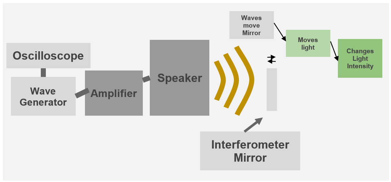
The phenomenon of interference allows the overall light intensity produced by waves to change based on the positions of the mirrors reflecting the waves. Since sound can alter these positions, it is possible to track sound effects through light intensity changes.

This experiment uses a Michelson interferometer, an instrument that employs a laser and multiple optical elements to recombine light, altering the output intensity¹². The sensitivity of the interferometer is strongly constrained by the mirror’s mass, mount resonance, and damping, which determine whether the optical elements can respond with sufficient displacement at 70–100 Hz. In this setup, a laser targets a half-silvered mirror (beam splitter), directing half of the beam to a mirror at a 90-degree angle and the other half to a mirror directly across from the laser (Fig. 1). The laser hits the surface and reflects. Based on the distance of the mirror, the reflected beams recombine at the beam splitter, creating constructive or destructive interference based on the mirror distances¹³. If a mirror oscillates by ¼ of the wavelength, the total distance traveled by the wave amounts to ½ wavelength, causing an oscillation in intensity that visually represents the sound wave (Fig. 2). The high sensitivity of the interferometer, often responding to movements of just tens of nanometers, makes it ideal for this experiment. However, this interpretation assumes a perfectly linear system and exact optical alignment. In practice, multiple interfering waves and small misalignments can obscure the clean sine pattern that the ¼ wavelength shift is expected to produce.

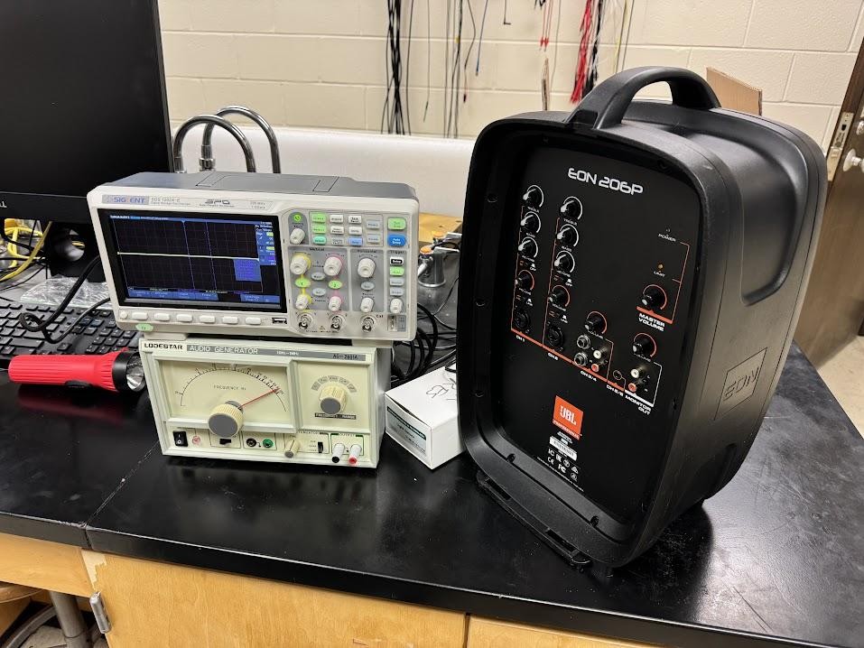
Interferometer Diagram (Top View)

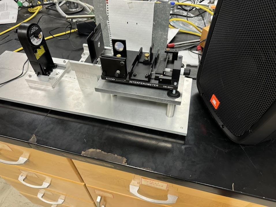
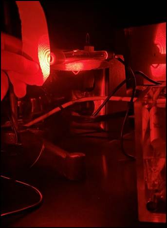
In this experiment, a loudspeaker generates sound waves at different frequencies, which are applied to a Michelson interferometer (PASCO Introductory Interferometer System) illuminated by a 515-nanometer green laser (Fig. 4). The loudspeaker (JBL EON206P) was positioned at approximately 15 cm from the interferometer at mirror height to maximize coupling. No mechanical coupling was applied; only acoustic waves drove mirror displacement. A Vernier light sensor (LS-BTA), aligned to capture only the central light beam, measures the resulting light intensity (Fig. 6). An oscilloscope reads a wave generator, which is connected to an amplifier and speaker to control the sine waves produced (Fig. 3). The Vernier light sensor samples the intensity every millisecond, providing detailed waveforms over 0.1 seconds and broader waveforms over 10 seconds. It samples up to 1,000 points per second (i.e. 1,000 Hz), so the test values of 70Hz, 80Hz, 90Hz, and 100Hz will be sufficiently captured by the sensor. The experiment exposes the instrument to these signals (with an error margin of ±0.09 Hz) to investigate the interference pattern’s light intensity and attempt to recreate the sound as light. Recording videos of the effects of the sound was considered and is another valuable way to collect the same data while showing the number of rings expanding in and out. Regardless, due to the low frame rate of the available camera, the method was discarded. In hindsight, however, even with low temporal resolution, techniques such as frame averaging or Fourier analysis could have extracted useful qualitative evidence of interference pattern changes, suggesting that video should not be dismissed outright.

The Vernier light sensor’s readings are recorded and processed using a LabQuest 2 device, which converts the signal into a text file and saves it onto a flash drive. The sensor samples 1,000 times per second. The data is then transferred to a laptop and converted into a CSV file. Using a custom program in a Python (Pyodide) Jupyter Notebook, a power spectral analysis was performed on the data to determine the average frequencies. With the 1,000 samples per second rate, the highest detectable frequency is 500 Hz.

The program converts the CSV file of the light intensity pattern into a corresponding WAV sound file. The results of these conversions are then evaluated and documented to analyze the relationship between sound waves and light intensity variations. For such delicate optical measurements, additional controls are necessary to ensure reliability. Environmental factors such as vibration isolation and air currents, as well as calibration of mirror displacement against sound amplitude, should be accounted for. Furthermore, background noise measurements are needed to confirm that the observed intensity variations arise from the applied speaker signal rather than ambient vibrations or structural resonances within the apparatus. A control will be measured without sound from the frequency to remove any noise from the data, but the results were limited due to the lack of instrumentation and resources. This experiment does not directly equate light intensity fluctuations with acoustic pressure but instead demonstrates an indirect transduction mechanism, where sound-induced mirror vibrations alter optical path lengths and thereby modulate the detected light.

The methodology utilizes Python libraries such as pandas, matplotlib.pyplot, numpy, and scipy.signal. It begins by loading the desired CSV file into a Pandas DataFrame for time-series analysis of light intensity (lux). Visualizations include plotting the raw data and computing the power spectral density (PSD) using Welch’s method (signal.welch) to examine frequency components. To convert the data into an auditory format, utility functions (read_csv, normalize_data, write_wav) are employed, leveraging scipy.io.wavfile.write to create a WAV file. The methodology concludes with the auditory output displayed using IPython.display.Audio, providing both visual and auditory insights into the dataset.

Results

70 Hz Samples

70Hz 0.1 Second Signal: Light Intensity vs. Time

70Hz 0.1 Second Signal: Light Intensity vs. Frequency

80 Hz Samples

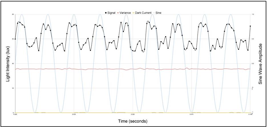
80Hz 0.1 Second Signal: Light Intensity vs. Time

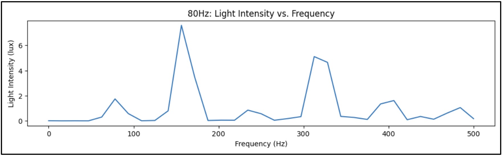
80Hz 0.1 Second Signal: Light Intensity vs. Frequency

90 Hz Samples

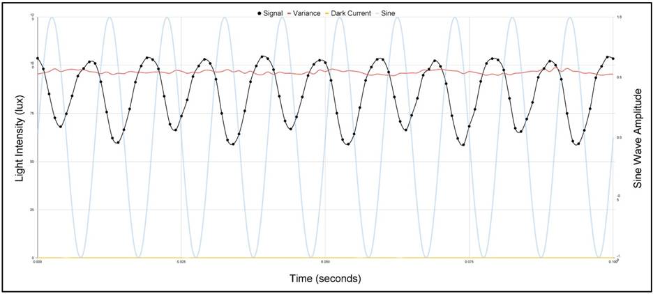
90Hz 0.1 Second Signal: Light Intensity vs. Time

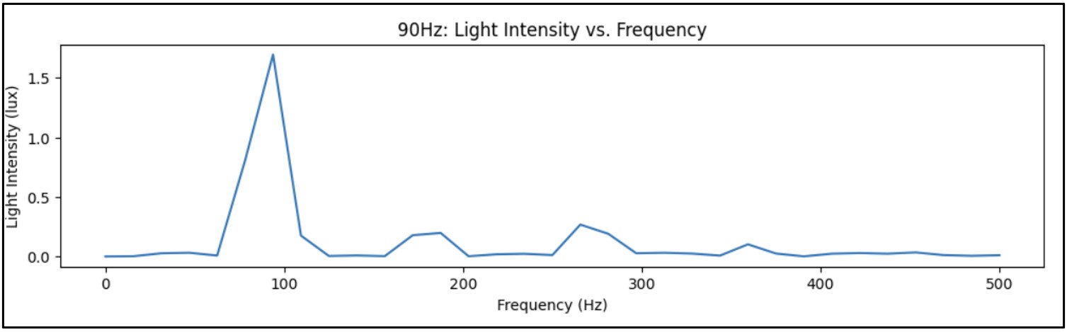
90Hz 0.1 Second Signal: Light Intensity vs. Frequency

100 Hz Samples

100Hz 0.1 Second Signal: Light Intensity vs. Time

100Hz 0.1 Second Signal: Light Intensity vs. Frequency

 Volume Effects on Waves

Volume’s Effect on Light Intensity Fluctuation

Volume’s Effect on Power Spectrums

Comparing the Sound From Light Intensity and the Sound from the Sine Wave

For the targeted frequencies, 10-second samples were taken at a sample rate of 1,000 samples per second. The 100Hz sample is used as an example to display the results.

100Hz 10-Second Sample: Light Intensity vs. Time

The actual 100 Hz wave is made from an online library of sine waves¹⁴. The following synthetic wave is made from the data points in Fig. 18.

Actual 100 Hz Wave:

https://drive.google.com/file/d/10TJBEXWQemsjjU1UVPuisvVZz5G6ARYC/view?usp=sharing

Synthetic 100 Hz Wave Produced from Light Intensity:

https://drive.google.com/file/d/1Pr9GpemfF-zbVUAOnq8PEZCmV4zPHRA9/view?usp=sharing

Discussion

This project demonstrated the feasibility of an interferometric optical microphone for sound detection. The system successfully detected acoustic signals in controlled settings, though challenges remain with background noise and sensitivity limits, especially in environments with significant vibration and air turbulence. Compared to piezoelectric microphones, the interferometric system showed higher immunity to electromagnetic interference but greater susceptibility to alignment drift and optical noise.
Several key findings emerged. First, while the system was able to detect fundamental tones reliably, harmonic resolution was inconsistent, reflecting limitations in sensitivity and optical stability. Second, although the design reduced susceptibility to electrical interference, external mechanical vibrations significantly affected performance. Finally, the project highlighted the broader potential of optical methods in assistive technologies for hearing loss. Existing aids such as vibrotactile devices and visual substitution tools provide valuable alternatives, but optical microphones could introduce new levels of sound fidelity and robustness.

Power spectral analysis further elucidated the relationship between sound frequencies and light interference patterns. By analyzing the power spectra of 0.1-second samples, inconsistencies and harmonics in the data are identified. Despite these inconsistencies, the presence of harmonics—which produce the same note at different octaves—indicates that sound reproduction from light interference remains feasible, although the system appears to be nonlinear¹⁵.

This reinforces the potential of using light interference frequencies as a novel method for sound detection and identification. Additionally, when comparing all of the frequencies’ power spectrums, each exhibited strength in different harmonics based on the frequency played. The instrument and experiment proved to be more complex than previously thought. Though the reasoning behind these patterns is unknown, it is a novel observation that has not been previously recognized. Due to the seemingly nonlinear nature of the interferometer interacting with sound, further experiments with more complex and layered sounds could be used to explore the possibility of representing voices to the hearing-impaired community¹⁶.

Overall, the findings of this study contribute to the field of optical sensing technologies. By demonstrating the ability to decode sound-induced vibrations from light patterns, this research lays the groundwork for innovative applications in assistive technologies for individuals with hearing impairments. The implications of accurately constructing light using sound are vast, offering new possibilities for enhancing accessibility in various environments.

70Hz Signal

The 70Hz signal initially became very bright, then gradually lost intensity at a slower rate. This signal produced a light-intensity wave with prominent even harmonics, resulting in non-uniform sine wave variations. Despite not forming perfect sine waves, the pattern consistently repeated according to the frequency’s period (Fig. 8). The interferometer primarily displayed higher even harmonics (Fig. 9), and the fundamental harmonic was much weaker than expected and difficult to resolve above the noise floor. Signals at even harmonics (140Hz, 280Hz, 420Hz) trended downward. The 70 Hz signal produced a signal-noise ratio (SNR) of -40.67 dB, supporting that noise caused nonlinear imperfections in the data collection.

80Hz Signal

The 80Hz frequency data provides a light fluctuation of minor and major ups and downs forming two parts of the wave that repeat throughout 80Hz (Fig. 10). This repeating “two-part” structure could indicate beating or amplitude modulation effects arising from reflections or coupling in the system. Although the pattern resembles the 70Hz data in some respects, the waveform remains distinctly different.

The 80Hz frequency data shows light fluctuations with minor and major peaks, forming a repeating two-part wave (Fig. 10). The sine wave of this frequency has also been graphed, revealing an overall peak pattern similar to the 70 Hz signal. Despite these similarities, the 80Hz signal has a distinctly different waveform than the 70 Hz light fluctuation wave.

The 80Hz power spectrum highlights the even harmonics, with the odd harmonics also present (Fig. 11). As the frequency increases, the intensity of light per even harmonic decreases, while the intensity of odd harmonics seems to increase. Although this pattern is suggested, there is not enough data to confirm it conclusively. Signals were found at the fundamental harmonic and other odd harmonics, trending upwards as the frequency increased. In contrast, even harmonics, initially more intense than odd ones, tend to decrease in intensity. The 80 Hz signal resulted in an SNR of -39.08 dB, supporting that noise produced significant changes in the data collection.

90Hz Signal

At the frequency of 90Hz, the graph starts to become less chaotic but is still not a perfect sine wave. It can be observed that the waveform is less drastic compared to 80Hz (Fig. 10) and that it also follows the pattern based on its sine wave’s period (Fig. 12). The sine wave of the frequency has also been graphed. The waveform displays two pairs of smaller peaks with one pair more intense than the other. Both of these peaks repeat as time moves forward. Similar to the previous frequencies, the peaks seem to follow a wave as well.

There is a large spike in the power spectrum at its fundamental harmonic while the rest of its harmonics up to the fourth are around the same lower level (Fig. 13). The 90 Hz frequency exhibits a better transition from sound to light compared to the 70 Hz and 80 Hz signals since its non-fundamental harmonics are weak while its fundamental is strong. There is a strong signal found at the fundamental harmonic while second to fourth harmonics are present but weak. On the other hand, even harmonics start as more intense than the odd ones but trend downwards. The 90 Hz frequency had an SNR of -38.05 dB, supporting that noise produced some changes in the data collection.

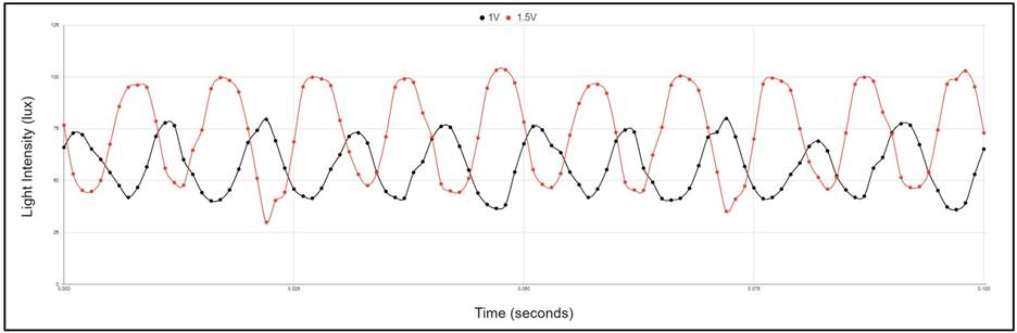
Effect of Volume on Light Intensity

When testing at 100Hz, the limited two-voltage comparison (1V and 1.5V) suggested that intensity changed while the waveform shape remained visually similar (Fig. 16). However, without a full voltage sweep, no firm conclusion can be made about waveform invariance under volume changes.

100Hz Signal

At 100Hz, the waveform is almost a perfect sine wave (Fig. 14). Just as the wave is almost a sine wave, the power spectrum also displays an almost pure signal at just 100Hz with no harmonics (Fig. 15). The imperfections are likely due to the sound’s inability to shift the interferometer’s mirror by the full 128.75 nanometers (or 1/4th of the wavelength).

Because of these details at 100Hz, it cannot be definitively ruled out that harmonics at lower frequencies are partially due to noise or system instability. A control run (no input signal) would be necessary to distinguish true harmonics from background artifacts. There is a strong signal found at the fundamental harmonic with no other signal present. There is a small half-harmonic in the power spectrum, but as stated before, it is likely due to the complexity and sensitivity of the interferometer. The 80 Hz signal produced a more accurate SNR of -18.9 dB, supporting that the sound could accurately trace harmonics when noise is less present.

Patterns of Waveforms

This experiment highlighted the use of the Michelson interferometer and sound almost as a synthesizer where the different harmonics are made more apparent depending on the frequency of moving the optical elements in the instrument. The fluctuations in light intensity were irregular but repeated in uniform. This is suggestive of nonlinear behavior where one or more elements could shift slightly, giving the outcome to be slightly different due to changes in the position of multiple elements¹⁵. However, no quantitative measures of nonlinearity (e.g., bifurcation diagrams, THD, RMS deviation from an ideal sinusoid, or cross-correlation with a reference sine) were performed, so this interpretation remains tentative. In further research, it is crucial to ensure the data is reproducible with little changes occurring between experiments. The range should also be altered to widen what frequencies that can be detected. Systematic frequency response testing across a broader acoustic range (beyond 70–100 Hz) is essential to characterize fidelity and establish harmonic behavior.

For instance, the 100 Hz wave initially expands towards a bright spot and then a dark spot. However, the sound from the speaker does not move all the way to complete darkness before it starts to contract. As it contracts, it must follow the same path backward, creating a mirror effect in its waveform as time continues to move forward.

Mirror Effect of Interferometric Light Fluctuation

This hypothesis is not the definitive conclusion for the behavior of the waves. No explicit time-reversal or spatial reflection tests were performed, so the attribution of symmetry to a mirror effect remains speculative. The complexity of the system or the coupling of the speaker to the interferometer might also contribute to this phenomenon. Initially, the study was planned to direct the speaker at one mirror to reduce sound effects on other elements of the machine, but time and resource constraints prevented this test from being conducted. Additionally, the complexity and non-linear nature of the experiment, akin to the butterfly effect, mean that slight movements in many system parts could affect the waveform formation. Due to these factors, it is challenging to determine why the waveform formed as it did.

Each of the waves’ peaks also follows a sinusoidal pattern (Fig. 20). This is due to the fact that each wave exhibits its frequency but at differing harmonics. However, because only four frequencies (70–100Hz) were tested, any inference about systematic odd/even harmonic behavior should be treated as a preliminary observation rather than a confirmed trend. A larger dataset across a wider frequency range would be required to establish robust conclusions.

Sound Reconstruction

The comparison between the original sine wave-generated audio and the light-based audio highlights the fidelity of our sound reconstruction technique, despite the inherent complexities introduced by harmonics. This validation solidifies the potential of optical sensing technologies for precise sound detection and reproduction in various applications.

Future Research

Future research should move beyond general speculation toward carefully designed experiments that provide measurable outcomes. One important next step is to address noise reduction and environmental stability. While this study showed that the interferometric microphone is less susceptible to electromagnetic interference than traditional devices, its vulnerability to mechanical vibrations and air currents limits reliability. Controlled experiments introducing specific environmental noise sources, such as vibration platforms or airflow disturbances, could help quantify tolerance thresholds and evaluate mitigation strategies, including vibration isolation or optical stabilization methods.

A second area of focus involves improving harmonic detection and signal processing. The inconsistencies observed in the current system’s power spectra suggest that sensitivity and resolution must be enhanced before the technology can reliably reproduce complex sounds¹⁷. Systematic testing across a broader frequency range, using standardized audio tones at varying amplitudes, would allow a full characterization of harmonic fidelity¹⁸. Additionally, advanced signal processing methods, including machine learning–based filtering and denoising algorithms, could be explored to separate true acoustic signals from optical noise, thereby increasing accuracy.

Finally, translational research should assess the feasibility of integrating interferometric microphones into assistive technologies for the hearing-impaired. Prototype systems could be developed to pair optical microphones with existing vibrotactile or visual substitution devices, allowing real-time acoustic-to-visual or acoustic-to-tactile conversion^19,20. Pilot testing with simulated hearing-impaired users would provide valuable insight into usability, latency, and real-world effectiveness. By linking laboratory experimentation with applied user testing, such work would establish whether this optical sensing approach can evolve into a clinically viable technology²¹.

Conclusion

This study explored the potential of detecting sound frequencies through light interference patterns in a Michelson interferometer. Preliminary results demonstrated that sound-induced vibrations can indeed be observed optically, though imperfections in waveforms and inconsistencies in power spectra indicate that reliable sound reconstruction has not yet been achieved. These findings suggest that while harmonics and frequency-dependent behaviors can be detected, the lab equipment and apparatuses used were limited in fidelity and scope.

Despite these constraints, the results establish a foundation for future work aimed at improving accuracy and extending the frequency range. With further validation, this approach could support the development of optical sensing technologies that benefit the hearing-impaired, such as systems providing visual or vibrotactile alerts in response to environmental sounds. By showing that acoustic information can be represented in optical signals, this research opens a pathway toward innovative assistive devices that may one day transform how individuals with hearing loss perceive and interact with their surroundings.

Acknowledgment

This work would not have been able to conduct my research with an interferometer nor understand the reasoning behind the data without the guidance of Dr. John M. Kenney. Thank you for your foundational lessons on interference and the principles of the research process that made this project possible.

I would like to acknowledge Dr. Mark Sprague for helping me with code and introducing me to IDEs such as Google Colab and Jupyter Notebook which made this project possible.

I would like to recognize Ms. Holly Choma for helping me with writing and organizing my paper along with teaching me and guiding me through equipment.

This project could not have been achieved without the encouragement and feedback of my classmates: Nachammai Annamalai and Felice Zhu.

Finally, this project would not have been made possible without the support of my family: Simon Huang, Karen Huang, and Tea Huang.

References

1. Z. Choudhary, G. Bruder, G. Welch. Visual hearing aids: Artificial visual speech stimuli for audiovisual speech perception in noise. Proceedings of the ACM on Human Computer Interaction. Vol. 7, pg. 1–18, 2023, https://doi.org/10.1145/3611659.3615682. [↩] [↩]
2. World Health Organization. Deafness and hearing loss, 2025, https://www.who.int/news-room/fact-sheets/detail/deafness-and-hearing-loss. [↩]
3. G. Kbar, A. Bhatia, M. H. Abidi, I. Alsharawy. Assistive technologies for hearing and speaking impaired people: A survey. Disability and Rehabilitation Assistive Technology. Vol. 12, pg. 3–20, 2017, https://doi.org/10.3109/17483107.2015.1079651. [↩]
4. S. Kochkin. MarkeTrak V: Why my hearing aids are in the drawer: The consumers’ perspective. The Hearing Journal. Vol. 53, pg. 34–41, 2000, https://doi.org/10.1097/00025572-200002000-00004. [↩] [↩]
5. B. Ohlenforst, A. A. Zekveld, E. P. Jansma, Y. Wang, G. Naylor, A. Lorens, T. Lunner, S. E. Kramer. Effects of hearing impairment and hearing aid amplification on listening effort: A systematic review. Ear and Hearing. Vol. 38, pg. 267–281, 2017, https://doi.org/10.1097/AUD.0000000000000396. [↩]
6. Cleveland Clinic. Hearing aids: Uses and how they work, 2023, https://my.clevelandclinic.org/health/treatments/24756-hearing-aids. [↩]
7. The Editors of Encyclopedia Britannica. Interference, 2024, https://www.britannica.com/science/interference-physics. [↩]
8. J. V. Knuuttila, P. T. Tikka, M. M. Salomaa. Scanning Michelson interferometer for imaging surface acoustic wave fields. Optics Letters. Vol. 25, pg. 613–615, 2000, https://doi.org/10.1364/OL.25.000613. [↩]
9. D. Brown, T. Macpherson, J. Ward. Seeing with sound? Exploring different characteristics of a visual to auditory sensory substitution device. Perception. Vol. 40, pg. 1120–1135, 2011, https://doi.org/10.1068/p6952. [↩]
10. R. Machorro, E. C. Samano. How does it sound? Young interferometry using sound waves. The Physics Teacher. Vol. 46, pg. 410–412, 2008, https://doi.org/10.1119/1.2981287. [↩]
11. E. Picou, T. Ricketts, B. Hornsby. How hearing aids, background noise and visual cues influence objective listening effort. Ear and Hearing. Vol. 34, pg. 1–12, 2013, https://doi.org/10.1097/AUD.0b013e31827f0431. [↩]
12. Caltech, MIT. What is an interferometer? https://www.ligo.caltech.edu/page/what-is-interferometer. [↩]
13. Y. Oikawa, M. Goto, Y. Ikeda, T. Takizawa, Y. Yamasaki. Sound field measurements based on reconstruction from laser projections. ICASSP. IEEE International Conference on Acoustics, Speech and Signal Processing. Vol. 4, pg. 661–664, 2005, https://doi.org/10.1109/ICASSP.2005.1416095. [↩]
14. Media College. Download audio tone files, https://www.mediacollege.com/audio/tone/download/. [↩]
15. J. P. Higgins. Nonlinear systems in medicine. The Yale Journal of Biology and Medicine. Vol. 75, pg. 247–260, 2002, https://www.ncbi.nlm.nih.gov/pmc/articles/PMC2588816/. [↩] [↩]
16. F. Bunkin, Y. Kravtsov, G. Lyakhov. Acoustic analogues of nonlinear optics phenomena. Soviet Physics Uspekhi. Vol. 29, pg. 607–633, 1986, https://doi.org/10.1070/PU1986v029n07ABEH003458. [↩]
17. I. V. Kaznacheev, G. N. Kuznetsov, V. M. Kuz’kin, S. A. Pereselkov. An interferometric method for detecting a moving sound source with a vector scalar receiver. Acoustical Physics. Vol. 64, pg. 37–48, 2018, https://doi.org/10.1134/S1063771018010104. [↩]
18. A. Haigh, D. Brown, P. Meijer. How well do you see what you hear? The acuity of visual to auditory sensory substitution. Frontiers in Psychology. Vol. 4, pg. 330, 2013, https://doi.org/10.3389/fpsyg.2013.00330. [↩]
19. R. P. Machado, D. Conforto, L. Santarosa. Sound chat: Implementation of sound awareness elements for visually impaired users in web based cooperative systems. International Symposium on Computers in Education. Vol. 2017, pg. 1–6, 2017, https://doi.org/10.1109/SIIE.2017.8259677. [↩]
20. M. Richardson, J. Thar, J. Alvarez, J. Borchers, J. Ward, G. Hamilton Fletcher. How much spatial information is lost in the sensory substitution process? Comparing visual, tactile and auditory approaches. Perception. Vol. 48, pg. 1079–1103, 2019, https://doi.org/10.1177/0301006619873194. [↩]
21. R. L. Goode, G. Ball, S. Nishihara, K. Nakamura. Laser Doppler vibrometer (LDV). The American Journal of Otology. Vol. 17, pg. 813–822, 1996. [↩]