Explainable Machine Learning Models to Predict Endurance of Athletes

Abstract

Aerobic and anaerobic thresholds (AeT and AnT) are key physiological determinants of an athlete’s performance, providing critical guidance for athlete’s training prescription, load management and competition strategy. This study investigates the efficacy of ensemble-based machine learning models in predicting AeT and AnT by capturing complex, individualized patterns within exercise data collected from athletes. We take a methodical, scientific approach building on the works of Tomaszewski et al. (2024)¹. We work with four ensemble algorithms, Random Forest, Extra Trees, XGBoost, and LightGBM, and systematically optimize through hyperparameter tuning, bootstrap-based confidence interval estimation followed by non-parametric significance testing and feature impact. The models demonstrate strong and consistent performance across training and testing datasets, indicating minimal overfitting. XGBoost achieved the highest predictive accuracy, with AeT R²_test = 0.814 (±0.135) and AnT R²_test = 0.923 (± 0.076) and outperformed previous work models. Results from the Nadeau–Bengio corrected t-test indicate that while all ensemble models achieved comparable R² scores, XGBoost significantly outperformed Random Forest and showed marginally higher performance, though not statistically significant than Extra Trees and LightGBM. Compared with prior work by Tomaszewski et al. (2024), which employed similar ensemble approaches on the same dataset, our models demonstrated improved generalization performance, particularly in R²_test scores. With SHAP analysis, we conclude that cardiovascular and metabolic features—particularly heart rate and lactate concentration are the most influential predictors, while anthropometric and demographic variables contribute minimally. These findings highlight the potential of ensemble learning approaches for accurate, individualized estimation of physiological thresholds for athletes and underscore their value in advancing adaptive training optimization and injury risk mitigation.

Keywords: sport, aerobic, anaerobic, thresholds, endurance, athletes, heart rate, lactate, machine learning, feature engineering, hyperparameter tuning, feature importance analysis, shap analysis

Introduction

Athletes, both professional and amateur, dedicate extensive time and effort to enhancing their performance through structured and rigorous training. A key focus of athletic conditioning is the development of endurance and efficiency, often achieved through cardiovascular training designed to elevate the aerobic (AeT) and anaerobic (AnT) thresholds—physiological markers that define an athlete’s capacity to sustain high-intensity efforts. These thresholds play a key role in planning an athlete’s workload, injury prevention and recovery to maximize on-field performance and career longevity.

The Aerobic Threshold (AeT) is the exercise intensity at which the body begins to noticeably increase its reliance on aerobic metabolism to supply energy. Below this point, energy is produced mainly using oxygen, and lactate production is low and stable. Training around the AeT helps build endurance, fat metabolism and trains the body to efficiently use oxygen. 

The Anaerobic Threshold (AnT) is the exercise intensity at which lactate begins to accumulate in the blood faster than the body can clear it. This marks the shift toward greater reliance on anaerobic metabolism. Above this point, fatigue sets in more quickly, and the effort cannot be sustained for long periods. Training near or just below the AnT improves the body’s ability to tolerate and clear lactate, allowing athletes to sustain higher intensities for longer periods. 

Together, Aerobic and Anaerobic thresholds demarcate 5 training zones that are used in coaching and training. Zone 1 is easy, recovery-level exercise, performed well below the AeT. Here the effort seems light, breathing is relaxed and fat is the dominant source of fuel². Just below AeT is Zone 2: here fat based metabolism is maximised and the breathing is steady. Training in this zone builds athletes’ aerobic capacity and long term endurance³. Zone 3 lies in between AeT and AnT thresholds. Here, the intensity feels moderately hard, the lactate levels are elevated but stable and both fat and carbohydrates are burned for fuel. Training in this zone increases stamina and enhances the body’s ability to clear lactate⁴.  Zone 4 is around AnT where exercise feels hard yet sustainable for limited durations. The body starts burning more carbohydrates for energy and lactate accumulates⁵. Above AnT, in Zone 5, the demand for oxygen reaches or exceeds maximal oxygen uptake, the breathing is very heavy and training in this zone is key for improving maximal aerobic power and anaerobic capacity⁶.

Thus, accurate prediction of AeT and AnT is critical to an athlete’s performance optimization as well as long term health maintenance. Even during games, a coach can use an athlete’s energy level and AeT/AnT thresholds to decide when to substitute a player or change strategies.

The determination of heart rate zones is a key aspect of training and is traditionally based on exercise intensity, as outlined by the American College of Sports Medicine⁷, or on measures such as maximum heart rate, heart rate reserve, or oxygen uptake reserve^8,9,10. These methods however, present limitations, particularly in estimating maximum heart rate. The commonly used age-based formula is imprecise, with a standard deviation of ±10–12 bpm, and tends to overestimate maximal HR in younger individuals while underestimating it in older adults⁹. 

Qualitatively, AeT is typically identified on the lactate curve as the point where values begin to deviate from the resting baseline, whereas the AnT corresponds to the stage of accelerated lactate accumulation. The most widely used analytical technique for determining AnT is the D-max approach. This method involves drawing a straight line between the first and last lactate measurements obtained during a graded maximal exercise test and identifying the point on the lactate curve that lies furthest from this line⁹. Determining these thresholds requires trained experts to interpret exercise data which makes it out of reach for many aspiring athletes¹¹. 

Machine learning (ML) models are highly suited for predicting AeT and AnT. These can handle complex, high dimensional data, analyse and learn from diverse datasets containing both physiological and performance data. ML Models can also work on data collected from disparate sources, including training logs, biometric sensors and external factors like weather to make the predictions more accurate.

The primary objective of this study is to develop and evaluate machine learning models capable of accurately predicting aerobic and anaerobic thresholds (AeT and AnT) using multimodal physiological and performance data, replacing the need for manual expert interpretation of lactate and heart rate charts. Additional objective is to understand the contribution of demographic and physiological factors including cardiovascular, respiratory and metabolic, on AeT and AnT prediction. By leveraging ensemble-based approaches, the study aims to establish a data-driven, objective, reproducible and interpretable method for threshold determination that enhances consistency and efficiency in athletic performance analysis.

Related Works

Machine Learning in Sports Physiology

Machine learning (ML) methods are increasingly used in sports physiology to model exercise responses and predict key endurance markers such as aerobic and anaerobic thresholds (AeT and AnT), lactate dynamics, and maximal oxygen uptake (VO₂max). Early studies relied on regression-based models to describe relationships between physiological variables and exercise intensity¹². More recent work has demonstrated the value of ensemble and boosting algorithms in handling non-linear, high-dimensional data typical of physiological systems. Kobayashi et al. (2023)¹³ showed that gradient-boosted trees could accurately estimate oxygen consumption during graded exercise tests, while Sughimoto et al. (2023)¹⁴ used random forest models to predict lactate concentration from electromyography (EMG) and heart rate signals. These studies illustrate the promise of ML in complementing traditional laboratory assessments. Building on this literature, our work focuses specifically on treadmill-based heart rate and lactate data to predict AeT and AnT, applying a systematic ensemble comparison that includes various machine learning models.

Contemporary research increasingly emphasizes multimodal modeling — combining cardiovascular, metabolic, biomechanical, and environmental data to capture the multifactorial nature of endurance performance¹⁵. Such approaches have demonstrated superior generalization and robustness by leveraging complementary sensor modalities, including power, EMG, GPS, and heart rate variability. Ensemble algorithms are particularly well-suited for integrating heterogeneous physiological features while maintaining interpretability. While our current dataset focuses on structured treadmill-based physiological measures (heart rate, lactate, speed), the modeling framework we propose is readily extensible to multimodal contexts. This design supports future integration of additional biometric and environmental data sources for more comprehensive performance modeling.

Tomaszewski et al., (2024) conducted a research study where they enlisted 183 amateur athletes (147 men, 36 women) aged between 16 and 62 years (mean: 36.1, standard deviation: 10.84 years). The authors collected several measurements for each of the athletes and collected data during a graded-to-failure CardioPulmonary Exercise Test (CPET) performed on an electric treadmill. They used Random Forest, XGBoost, and LightGBM to predict an athlete’s AeT and AnT threshold values. However, their results show a striking difference between the quality of output for test vs train data; for eg, their trained Random Forest for AeT shows R²_train of 0.956 and R²_test of 0.645 – a deterioration of 33%. The same pattern holds for other models while predicting both AeT and AnT. We believe the model is likely overfitting training data rather than actually learning from it and thus performing poorly on test & unseen data. 

Explainable Machine Learning in Physiology

As ML models become more prevalent in physiological research, interpretability has emerged as a critical requirement for scientific and clinical credibility. Explainable AI (XAI) techniques such as SHAP¹⁶ provide transparent measures of feature influence, allowing physiological validation of model behavior. Recent applications in sports science have used SHAP or feature attribution to identify predictors of performance, fatigue, and recovery¹⁷. However, the adoption of explainable ML within endurance physiology remains limited, particularly for thresholds that reflect complex cardiovascular and metabolic interplay. Our study explicitly integrates SHAP-based interpretation to identify dominant predictors of AeT and AnT, such as heart rate and lactate concentration, providing physiological insight in addition to predictive accuracy.

Research Gap and Contribution

Despite these advances, few studies have systematically benchmarked multiple ensemble algorithms using rigorous hyperparameter tuning, repeated cross-validation, and uncertainty estimation in the context of endurance physiology. Furthermore, explainability remains underutilized as a means of validating ML models against physiological mechanisms. In this study, we attempt to address these gaps by (i) systematically comparing ensemble models under a statistically rigorous evaluation framework, (ii) quantifying model uncertainty using repeated cross-validation and bootstrap confidence intervals, and (iii) applying SHAP-based explainability to uncover the physiological determinants of aerobic and anaerobic thresholds from treadmill-based data.

Dataset

This research builds on the research and dataset from an anonymized physiological performance of amateur endurance athletes as described in Tomaszewski et. al (2024). The dataset consists of results from 183 participants, with a 147 to 36 split of men and women, respectively. Participants ranged from age 16 to 62 years old (mean: 36.1, standard deviation: 10.8 years). Each participant led an active life, training, on an average of 3-4 times per week in their respective disciplines. All participants were put through graded-to-exhaustion CaridoPulmonary Exercise Test (CPET) on a treadmill.

Athletes start with a 10 minute warmup and then run at 6 km/h, 8 km/h and 10 km/h successively on the treadmill for 3 minutes each. After this, the speed is increased by 2 km/hr every 2 minutes until the treadmill reaches a speed of 22 km/h. The test ends at 22 km/h or at volitional exhaustion (when the athlete can no longer maintain treadmill speed). These runs on the treadmill are without break.  During the test, respiratory indicators like ventilatory equivalent (VE) l/min and oxygen uptake (VO2) (l//min/kg) are measured. Blood is collected from the fingertip in the last 15 secs of each stage to measure lactate concentration. Data is recorded per athlete and later enhanced with computed values, such as la_min, la_max, hr_la_min, hr_la_max and speed_la_max. The recorded dataset consists of a mix of demographic, anthropometric, and physiological variables as shown in Table 1. The output target columns are both AeT and AnT, which represent the physiological thresholds used in endurance training. 

Variable Name	Description
AeT	Aerobic Threshold
AnT	Anaerobic Threshold
sex	male/female
date	Date of the recording
age	Age of the athlete
height	Height of the athlete
weight	Weight of the athlete
discipline	List of sports played by the athlete
vo2max	maximal oxygen uptake or an individual’s maximum capacity to take in oxygen during an intense exercise
vo2_at	oxygen consumption measured at the aerobic threshold
VE	Ventilatory Equivalent or total volume of air breathed in and out per minute
R	Restitution/Recovery (R) is the time taken for the post-exercise heart rate drop to 60% of the maximum heart rate achieved during the test
hrmax	Maximum heart rate
RF	Respiratory Factor (RF) indicates how much of the oxygen extracted from the lungs into the bloodstream
vo2max_l_m	maximal oxygen uptake measured in absolute terms (l/min), not relative to body weight.
hr_6 .. hr_22	Heart rate at speed 6 km/h to heart rate at speed 22 km/hr
la_6 .. la_22	Lactic acid level at speed 6 km/h to lactic acid level at speed 22 km/hr
la_min	calculated variable, minimum value of lactic acid for the athlete in the experiment
la_max	calculated variable, maximum value of lactic acid for the athlete in the experiment
hr_la_min	calculated variable, heart rate corresponding to minimum lactic acid level
hr_la_max	calculated variable, heart rate corresponding to maximum lactic acid level
speed_la_max	calculated variable, Treadmill speed at maximum lactic acid level

Methodology

Exploratory Data Analysis 

Tomaszewski, et al (2024) collected a rich set of data from their experiments.  Out of 183 participants, women constitute 36 (20%) and men 147 (80%). Not all attributes have values for all the observations because this is a graded-to-exhaustion. Some attributes had sparse data for e.g., hr_14 (heart rate at speed 14 km/h) and hr_16 have 5% and 23% data missing. Similarly, la_14 and la_16 have 12% and 44% of the data missing respectively. Some attributes have a much higher percentage of missing data. These include hr_18 (62% missing), hr_20 (89% missing), hr_22 (99% missing data), la_6 (100% missing), la_18 (72% missing), la_20 (92% missing) and la_22 (99% missing) as shown in Table 2. 

Variable	% Missing
hr_14	5%
hr_16	23%
hr_18	62%
hr_20	89%
hr_22	99%
la_6	100%
la_14	12%
la_16	44%
la_18	72%
la_20	92%
la_22	99%

Features with more than 50% missing values were excluded from the analysis in accordance with established recommendations for small biomedical datasets, as imputing variables with high missingness can introduce substantial noise and bias^18,19. This threshold is widely adopted in clinical and machine learning research to preserve data integrity when reliable reconstruction of missing information is not feasible. For the remaining variables with moderate missingness, (hr_14, hr_16, la_14, and la_16 as shown in Table 2), missing values were imputed using the K-Nearest Neighbors (KNN) method with 2 nearest neighbors, which leverages similarity between observations to estimate plausible replacements²⁰.

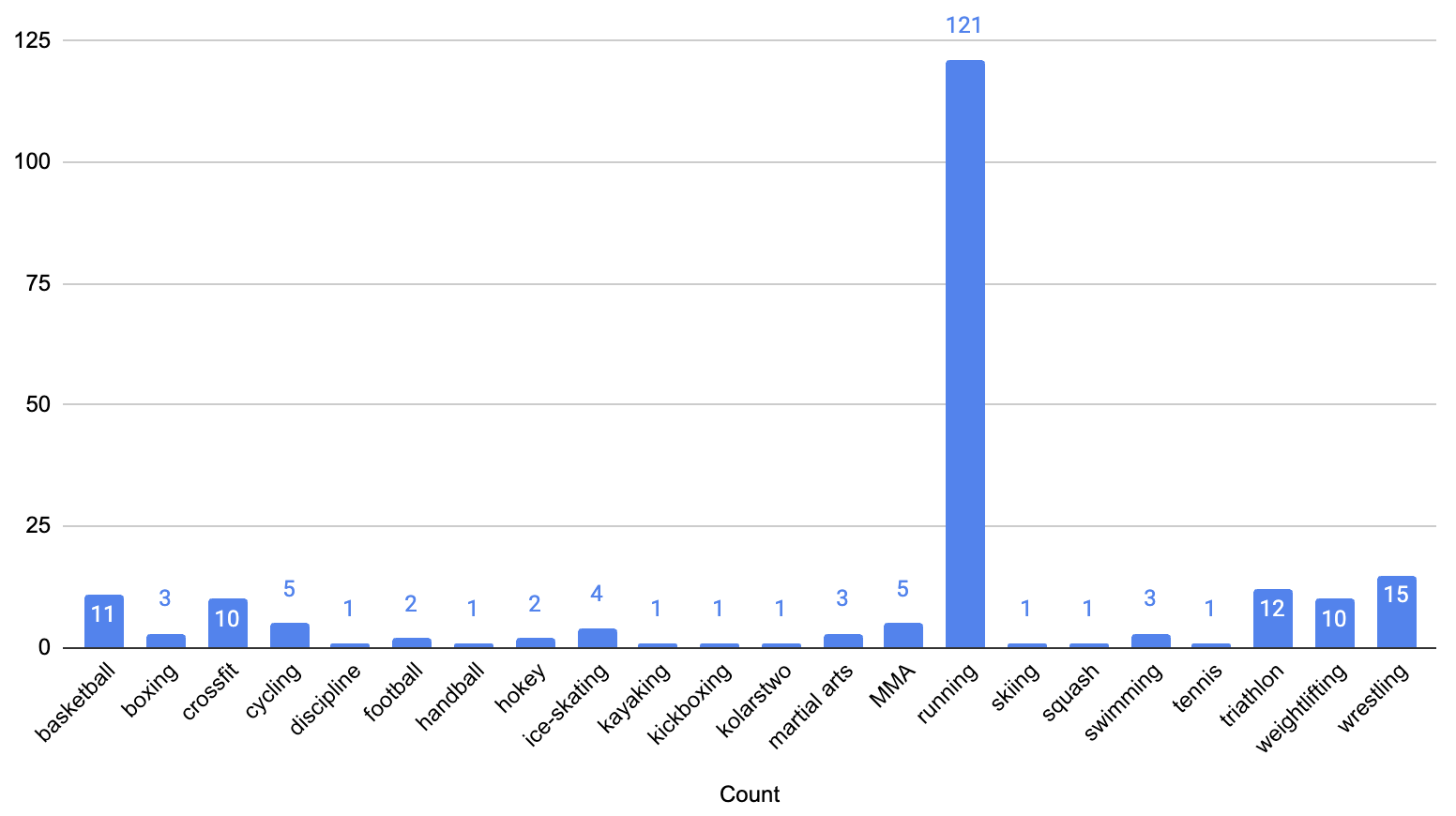
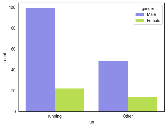
The feature ‘discipline’ contains a text list of sports the athlete plays. While 161 athletes reported playing one sport, 15 reported playing 2 sports, 6 reported playing 3 and one athlete reported playing 4 sports. Running was the most common reported sport (121 athletes) followed by wrestling (15) reported by ~8% of the participants as depicted in Figure 1. We converted discipline into a numerical form that models can understand. Since the CPET test involved treadmills and given other sports had very low participation, we decided to binary encode discipline by introducing a new attribute, sport and set its value to 1 if the athlete listed running as a sport and 0 if not. Among participants, 99 men (67% of all men) and 22 women (62% of all women) reported running (see Figure 2). The proportion of men to women who run (82% vs. 18%) closely reflects the overall gender distribution in the cohort (80% men vs. 20% women).

We analyzed demographic, anthropometric, and physiological variables as summarized in Figure 3. The athletes’ ages ranged from 16 to 62 years, with a mean of 36.1 years. Body weight varied between 39 kg and 111 kg (mean 74.9 kg), and height ranged from 155 cm to 205 cm (mean 176 cm), both approximating normal distributions. Resting heart rate spanned 75–161 bpm (mean 107.8 bpm), while maximum heart rate during exercise ranged from 148–212 bpm (mean 182.4 bpm). Lactic acid concentration at a treadmill speed of 8 km/h ranged from 1.0 to 12.1 mmol/L, with a mean of 3.4 mmol/L. The observed patterns reveal substantial inter-individual variability, particularly in heart rate (hr_6 and hrmax) and lactate (la_8) measures. The hr_6 distribution shows a right-skewed profile, suggesting a greater concentration of athletes with moderate cardiovascular capacity and fewer with exceptionally high endurance levels. Similarly, lactate concentrations display a right-skewed distribution, indicating greater concentration of athletes with small measures of lactates. The relatively normal distributions of anthropometric features (e.g., height, weight).

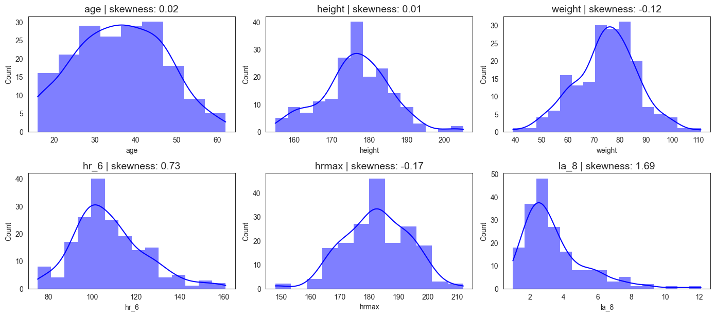
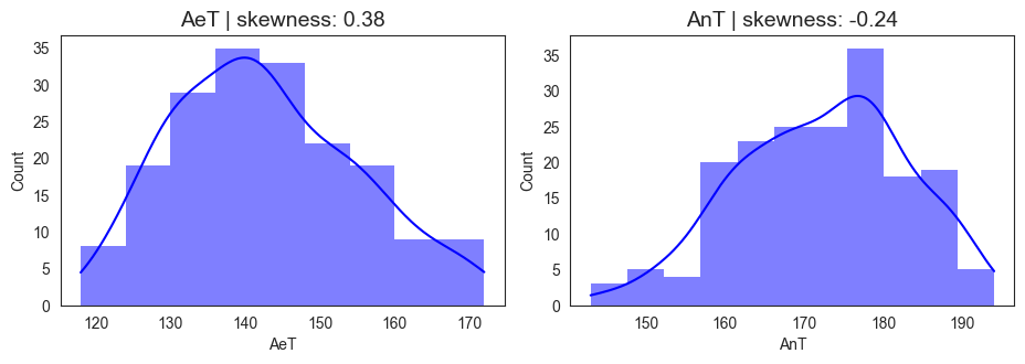
Figure 4 illustrates the distribution of aerobic (AeT) and anaerobic thresholds (AnT) among the athletes. AeT values ranged from 118 to 172 bpm, with a mean of 142.7 bpm and a slight positive skewness (0.38), indicating that while most athletes cluster around moderate AeT levels, a subset of athletes exhibits higher aerobic thresholds, potentially reflecting superior cardiovascular endurance or long term endurance training. AnT values ranged from 143 to 194 bpm, with a mean of 172.3 bpm and a slight negative skewness (-0.24), suggesting that most athletes reach their anaerobic threshold at relatively higher heart rates, but a few reach it earlier, possibly reflecting individual differences in lactate tolerance or training adaptation. The roughly 30 bpm gap between AeT and AnT represents the “aerobic–anaerobic transition zone,” a key marker of endurance performance. A narrower AeT–AnT gap often signifies greater metabolic efficiency and training maturity. The observed values, therefore, suggest that the cohort includes many well-trained individuals with robust aerobic foundations and efficient anaerobic responses.

The skewness patterns in AeT and AnT might reflect training status variation in the population. In total, 183 observations were recorded, highlighting substantial inter-individual variability in both thresholds despite a relatively homogeneous cohort. This variability underscores the importance of individualized threshold prediction rather than population-based estimation, as athletes exhibit unique physiological responses shaped by training history, genetics, and sport specialization, which underscores the need for personalized modeling approaches for performance prediction.

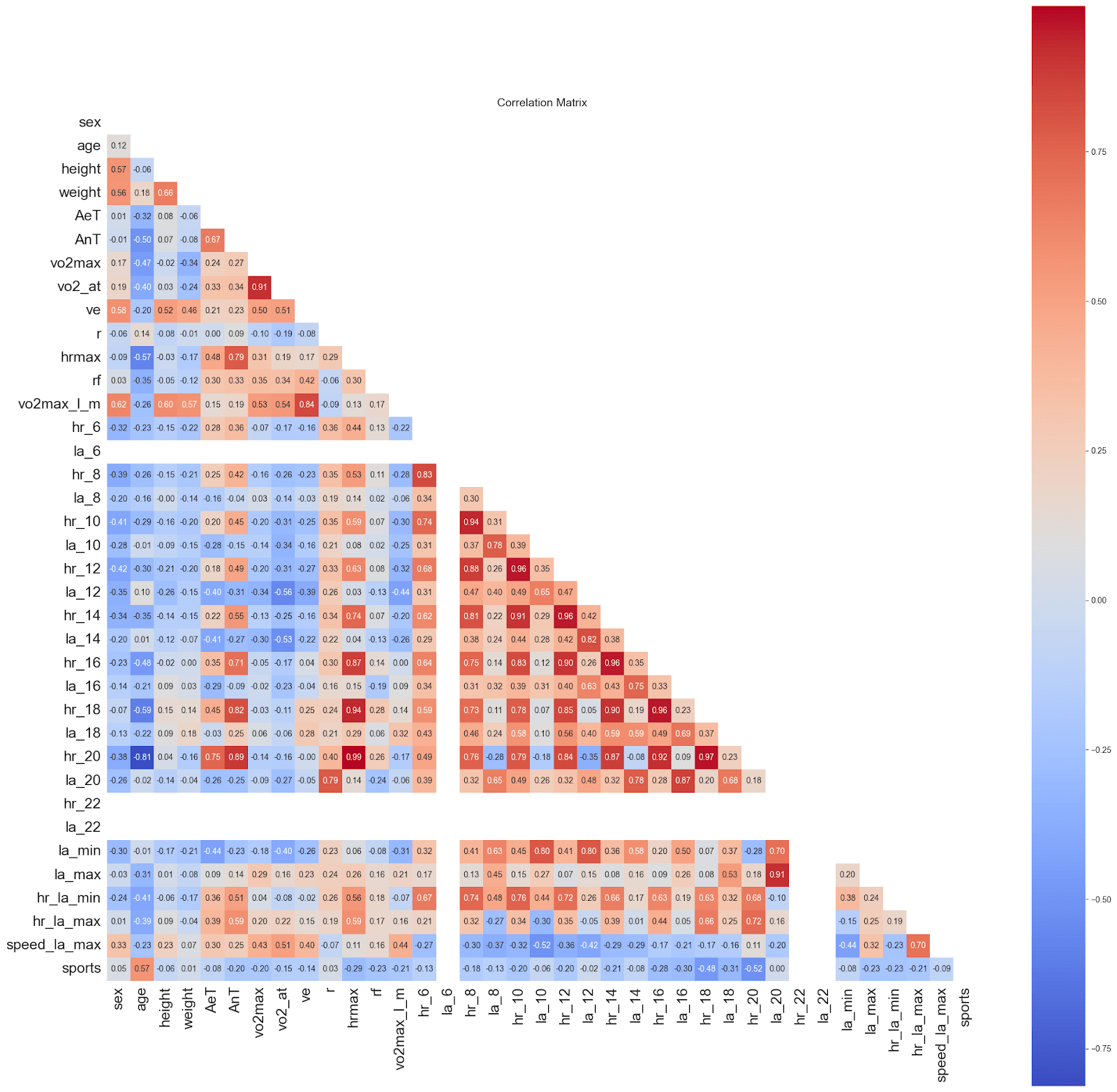
We examined the presence of collinearity in our dataset using a Pearson correlation matrix, as shown in Figure 5. Variance Inflation Factor (VIF) analysis in Table 3 indicates high collinearity among heart rate measurements at adjacent treadmill speeds.  Heart rates and lactic acid concentration responses to incremental workloads are inherently autocorrelated, reflecting continuous cardiovascular adjustment in the human body rather than redundant measurement. Consequently, these variables were retained, as their collective pattern across increasing speeds encodes essential information about aerobic and anaerobic thresholds. Similar approaches are standard in exercise physiology and biomedical modeling, where sequential physiological responses are jointly modeled despite high inter-feature correlation^3,21.

However, we excluded vo2_at (oxygen consumption measured at the aerobic threshold) from the predictor set, as it directly depends on the target variable being modeled. Since the goal of our study is to predict the aerobic and anaerobic thresholds, vo2_at would not be available at inference time and was therefore omitted to prevent data leakage.

Although retaining these physiologically correlated features does not compromise predictive performance, it can influence feature importance interpretation, as the contribution of individual variables may be distributed across correlated pairs. To address this, we apply domain-driven grouping to aggregate the effects of related predictors when interpreting model outputs, ensuring that the combined impact of related predictors is accurately represented and is physiologically meaningful.  

Rank	Variable	VIF	Category
1	dhr_la_max	91.308	Very High
2	hr_la_max	85.479	Very High
3	dhr_la_min	82.354	Very High
4	hr_la_min	80.635	Very High
5	dhr_14	59.773	Very High
6	dhr_12	59.636	Very High
7	dhr_10	37.384	Very High
8	dhr_16	34.305	Very High
9	speed_la_max	29.068	Very High
10	vo2max_l_m	18.867	High
11	weight	14.927	High
12	vo2max	13.949	High
13	dhr_8	8.465	Moderate
14	dla_min	7.898	Moderate
15	la_max	7.629	Moderate
16	hrmax	7.191	Moderate
17	dla_max	6.496	Moderate
18	la_min	6.377	Moderate
19	ve	6.113	Moderate
20	dla_12	5.887	Moderate
21	dla_14	4.322	Low
22	dla_10	3.688	Low
23	age	3.433	Low
24	dla_16	3.223	Low
25	height	2.703	Low
26	sex	2.566	Low
27	rf	2.095	Low
28	sports	1.74	Low
29	r	1.639	Low

Input Features and Output Target

Since athletes exhibited varying levels of cardiovascular fitness, heart rates at different running speeds were normalized by dividing each value by the individual’s baseline heart rate measured at 6 km/h.  Several prior studies have normalized heart rate (HR) responses relative to baseline to account for inter-individual variability in resting cardiac tone^22,23,24. Although normalization could alternatively be performed using the maximum heart rate or the heart rate at another reference speed, we selected heart rate measured at 6 km/h as the normalization factor because it represents a stable, low-intensity baseline condition that is comparable across subjects. Furthermore, in real-world or inference scenarios, athletes may not always complete the full treadmill protocol, and maximum heart rate data may therefore be unavailable. In contrast, baseline heart rate at the initial speed is consistently available, making heart rate measured at 6 km/ha more practical and a robust normalization reference. 

We applied a similar approach to lactic acid levels, where we normalized these based on their lactic acid levels at speed 8 km/hr. For lactic acid levels, we normalized to the levels of lactic acid at speed 8 km/h as the dataset did not have measurements of lactic acid at 6 km/h. As a precaution to prevent leakage, we removed hr_6 and la_8 from our model inputs. In addition to the above normalized heart rate and lactic acid  features, we use features such as sex, age, height, weight, ve, vo2_at, r, rf, hrmax, running as well as calculated variables la_min, la_max, hr_la_min, hr_la_max and speed_la_max as input to the model to predict  Aerobic (AeT) and Anaerobic (AnT) thresholds in athletes.

Models and Evaluation Metrics

We selected four ensemble-based machine learning algorithms—Random Forest (RF), Extra Trees (ET), XGBoost (XG), and LightGBM (LGBM) —based on prior literature as well as their demonstrated effectiveness in modeling complex physiological and biomedical data. The study builds upon the work of Tomaszewski et al. (2024), extending their framework by systematically tuning and evaluating a broader set of ensemble models, including the addition of Extra Trees for comparative completeness. Ensemble methods have shown superior performance in predicting physiological markers such as blood lactate concentration and oxygen uptake from electromyography and sensor data, outperforming linear regression and single-model approaches^25,26,12. Their ability to model non-linear relationships, manage structured and moderately sized datasets, and maintain interpretability through feature importance metrics (SHAP analysis) makes them particularly well-suited for endurance physiology. Prior studies have also demonstrated that ensemble approaches generalize effectively to unseen subjects in multimodal physiological prediction tasks¹⁵. While deep or hybrid neural architectures could capture higher-order dependencies, the focus of this study is on interpretable and robust modeling within a limited-sample, high-dimensional context. Accordingly, we adopted these four ensemble models to provide a balanced comparison between bagging-based (Random Forest, Extra Trees) and boosting-based (XGBoost, LightGBM) learning paradigms.

Random Forest is an ensemble method that builds multiple decision trees using bootstrap samples of the data and averages their predictions. It is known for its robustness to overfitting, ability to handle non-linear relationships, and interpretability through feature importance²⁷.

Extra Trees is similar to Random Forest but introduces additional randomness by selecting split points at random rather than searching for the most optimal split. This often leads to faster training times and, in many cases, comparable or better generalization performance, particularly on noisy datasets²⁸.

XGBoost (Extreme Gradient Boosting) is a gradient boosting algorithm that builds trees sequentially, each one focusing on correcting the errors of the previous. It is optimized for speed and performance, with features such as regularization and efficient handling of missing values, making it one of the most competitive models for tabular prediction tasks²⁹.

LightGBM (Light Gradient Boosting Machine) is another gradient boosting framework that uses a histogram-based algorithm and leaf-wise tree growth to achieve faster training and reduced memory usage. It is particularly well-suited for large datasets and high-dimensional features, offering a strong balance between accuracy and computational efficiency³⁰.

To evaluate model performance, the dataset was divided into training and test subsets. The training set was used for model fitting and hyperparameter optimization, while the test set was reserved exclusively for performance evaluation to ensure an unbiased assessment of generalization. An 80/20 train/test split was chosen as a practical tradeoff for small sample sizes, consistent with common practice in applied ML literature^31,32. Repeated cross-validation was used during model selection to mitigate variance due to the small dataset size. During hyperparameter tuning, cross-validation performance was assessed using Repeated 5-Fold cross-validation (10 repeats). To assess performance, we used multiple complementary metrics, such as R², mean absolute error (MAE) and mean absolute percentage error (MAPE). Choosing these metrics also allows us to compare our outputs and accuracy with the work of Tomaszewski, et al (2024) for an accurate and systematic comparison. 

Hyperparameter Tuning

To optimize model performance, hyperparameter tuning was performed using GridSearchCV³⁰ with 5-fold cross-validation repeated 10 times on the training set. GridSearchCV systematically evaluated combinations of these hyperparameters across the cross-validation folds, selecting the configuration that maximized predictive performance while minimizing overfitting. This approach ensures that each model operates under near-optimal conditions, providing a robust and fair comparison of predictive accuracy across algorithms. The selection of hyperparameter search ranges was guided by empirical evidence and recommendations in the literature for small to moderately sized datasets. 

For models with boosting-based approaches –  XGBoost and LightGBM, we worked with parameters n_estimators, learning rate, sub sample and colsample_bynode as shown in Table 4. n_estimators defines the number of trees in the forest. More trees usually improve stability and accuracy, as predictions are averaged over multiple models but it also increases computation times and may result in overfitting. We limited the number of boosting iterations (n_estimators) to 100–500 to balance model expressiveness and overfitting risk. Studies have shown that on small datasets, excessive boosting rounds (e.g., > 500) can lead to overfitting even with early stopping^29,30. Intermediate values (100, 300, 500) were selected to cover increments across a practical training range while maintaining computational costs³³. Learning rate shrinks the contribution of each new tree, controlling the step size in boosting updates. A smaller learning rate improves generalization and stability but requires more trees (higher n_estimators). Larger values speed up training but may cause overfitting or convergence to a suboptimal solution. We optimized over the following learning rates (0.001, 0.002, 0.003, 0.01, 0.02, 0.03, 0.1, 0.2, 0.3). The learning-rate grid (0.001–0.3) reflects commonly adopted search boundaries in prior work, where rates below 0.001 yield negligible incremental learning and those above 0.3 often produce unstable convergence or loss divergence on small datasets^2,34. Given our dataset size (n = 183), the finer granularity would not materially affect model selection but would substantially increase computational costs. 

The subsample hyperparameter controls the fraction of training instances randomly sampled (without replacement) to construct each tree. Using subsample values below 1.0 introduces stochasticity analogous to stochastic gradient descent, which helps reduce variance and prevent overfitting. However, excessively small values can increase bias and degrade model accuracy. Empirical studies and tuning guides recommend moderate subsampling values between 0.6 and 1.0 as an effective trade-off between generalization and bias^31,30,33. Accordingly, we optimized over (0.6,0.7,0.8,0.9,1.0), consistent with standard practice in ensemble-based boosting frameworks. Colsample_bynode (or feature subsampling per node) parameter specifies the fraction of predictor variables randomly chosen at each split. Feature subsampling further decorrelates trees, improving robustness and computational efficiency, particularly in high-dimensional feature spaces²⁹. As with subsample, tuning colsample_bynode within the range (0.6, 0.7, 0.8, 0.9, 1.0) is supported by prior literature and practical recommendations in both XGBoost and LightGBM documentation, where moderate subsampling (<1.0) has been shown to enhance generalization without substantially increasing bias. The chosen ranges therefore represent an evidence-based compromise between performance sensitivity and overfitting control for limited-sample gradient boosting.
For bagging-based ensemble models—Random Forest (RF) and Extra Trees (ET)—we optimized key hyperparameters, namely n_estimators, max_features, and min_samples_split, following standard recommendations in ensemble learning literature. The parameter n_estimators defines the number of trees in the ensemble. Increasing the number of trees typically enhances predictive stability and reduces variance by averaging across multiple decorrelated models, though excessively large ensembles can yield diminishing returns in accuracy and higher computational cost. Accordingly, we evaluated n_estimators  {100, 300, 500}, a range consistent with prior empirical studies and practical guidance for small- to medium-sized datasets^31,35. The min_samples_split parameter controls the minimum number of samples required to split an internal node. Smaller values permit deeper, more complex trees and increase the risk of overfitting, whereas larger values constrain tree growth and can introduce bias. We varied min_samples_split between 5 and 60 in increments of 5 to balance model complexity and generalization³⁵. Finally, max_features determines the number of predictors randomly selected for consideration at each split. This random feature selection decorrelates trees, enhancing generalization and reducing overfitting. Following standard practice of going as wide as possible, we explored max_features values from 1 to 30 (equal to the total number of available features)³⁵, incrementing by one, to systematically evaluate the trade-off between bias and variance under varying feature subsampling levels.

Model	Parameter	Value Range
Random Forest	n_estimators	100, 300, 500
	min_samples_split	between 5 and 60 with increment of 5
	max_features	between 1 and 30 with increment of 1
Extra Trees	n_estimators	100, 300, 500
	min_samples_split	between 5 and 60 with increment of 5
	max_features	between 1 and 30 with increment of 1
XGBoost	n_estimators	100, 300, 500
	learning_rate	0.001, 0.002, 0.003,0.01, 0.02, 0.03, 0.1, 0.2, 0.3
	subsample	0.6, 0.7, 0.8, 0.9, 1.0
	colsample_bynode	0.6, 0.7, 0.8, 0.9, 1.0
Light GBM	n_estimators	100, 300, 500
	learning_rate	0.001, 0.002, 0.003,0.01, 0.02, 0.03, 0.1, 0.2, 0.3
	subsample	0.6, 0.7, 0.8, 0.9, 1.0
	colsample_bynode	0.6, 0.7, 0.8, 0.9, 1.0

The model’s training performance was evaluated using a repeated 5-fold cross-validation (CV) with 10 repetitions, providing robust estimates of generalization while accounting for variability due to data splits. The reported metrics (R², MAE, and MAPE) include the mean value across folds ± the corresponding 95% confidence interval (CI), reflecting both the central tendency and the uncertainty of the estimate. Training confidence intervals are calculated using the percentile method on cross-validation scores from Repeated K-Fold validation. The 95% CI is defined by the 2.5^th and 97.5^th percentiles of R², MAE and MAPE scores obtained from different data folds. This approach mitigates overfitting and gives a more reliable picture of model stability than a single train/test split, as it captures the variance in performance across multiple partitions of the dataset. The confidence intervals allow us to quantify the expected fluctuation in performance due to sampling, offering insight into whether observed differences between models or hyperparameter settings are likely to be meaningful or simply due to random variation. Overall, these CV metrics with CI provide a balanced assessment of model accuracy and reliability on unseen data.

The model’s test performance was assessed using a bootstrap procedure with   5000 bootstraped resamples and a confidence level of 𝛼 = 0.05. This non-parametric approach estimates the distribution of the test metric by repeatedly sampling with replacement from the test set, allowing us to compute robust 95% confidence intervals around the point estimates. Performance metrics (R², MAE, and MAPE) were calculated for each iteration, generating distributions of each metric. Performance metrics are reported as mean ± margin of error, where the margin of error is half the width of the 95% bootstrap confidence interval, computed from 5,000 resamples using the percentile method. These provide an understanding of both the expected performance and its uncertainty due to sampling variability. By using a large number of bootstrap resamples, the analysis reduces the impact of random fluctuations in the test set, giving more reliable estimates than a single evaluation. This approach ensures that reported model performance reflects not only point estimates but also the uncertainty inherent in the dataset, which is particularly important for physiological measurements like lactate that may vary across training sessions and individuals.

Statistical Comparison (Nadeau & Bengio corrected t-test) of Models Differences

When evaluating machine learning models, it is insufficient to rely solely on raw performance metrics, as observed differences may arise from random variation in the data rather than true improvements. Statistical comparison methods are therefore necessary to determine whether performance differences between models are significant or merely due to chance³⁶.

To assess this, we applied the Nadeau & Bengio corrected t-test, which is specifically designed for performance comparisons under repeated cross-validation. This test accounts for the dependency between folds that arises in repeated 5-fold cross-validation, providing a more accurate estimate of variance than standard paired tests. In our study, the corrected t-test was applied to the distributions of absolute errors produced by each model (Random Forest, Extra Trees, XGBoost, and LightGBM) across repeated folds. By comparing the mean differences while correcting for overlap between training sets, the test evaluates whether one model consistently outperforms another. A p-value below 0.05 was considered evidence of a statistically significant difference in predictive performance³⁶.

Feature Importance Analysis 

Feature importance analysis helps transform a black-box model into a more interpretable tool, guiding feature selection, uncovering hidden insights, and building trust. Feature importance analysis is performed to understand which input variables contribute most to a model’s predictions. This is crucial as it improves model interpretability, helps debug and trust the model, guides feature selection to reduce dimensionality, and can even reveal domain insights that inform business or scientific decisions. This is a useful check in model development.

We use SHAP (SHapley Additive exPlanations) Analysis, a model-agnostic, theoretical method based on Shapley values from cooperative game theory, which attributes the contribution of each feature to a specific prediction¹⁶. It provides consistent and locally accurate explanations: the sum of SHAP values for all features equals the difference between the model output and the baseline expectation. This allows one to see not only which features are important overall, but also how each feature pushes a prediction higher or lower for an individual instance. When doing SHAP analysis, to obtain more meaningful insights, we applied domain-driven grouping of related variables. We chose conceptual rather than algorithmic grouping – statistical or clustering-based aggregation – with an intent to enhance interpretability. Such domain-based SHAP aggregation has been adopted in prior physiological modeling research³⁷, where features were grouped by biomedical relevance to improve interpretability without compromising fidelity. We grouped all heart rate related features (e.g., heart rates at different treadmill speeds, hr_la_max, hr_la_min, hrmax, etc.) into a group called heart rate (hr). Similarly, we grouped lactate level related features (e.g. lactic acid concentration at different treadmill speed, la_min, la_max) into a group called la. The grouping was therefore conceptual and additive: the sum of mean absolute SHAP values within each group so as to facilitate interpretability at the physiological domain level without modifying the underlying SHAP attributions. This helps us ascertain the true impact of heart rate, lactic acid levels and other predictors in the prediction of AeT and AnT.  

Results and Discussion

We use demographic, anthropometric, and physiological data and a set of chosen models to train and predict an athlete’s AeT and AnT. Along with each prediction, we also record various evaluation metrics and confidence intervals. This helps us compare the models objectively amongst themselves and with previous work. We follow this up with feature importance analysis as well as evaluate if each of the model output is statistically significantly different from one another. 

Results for Aerobic Threshold  

For AeT the model performance is shared in Table 5. For each of the models we achieve a strong R² value with tight confidence interval and relatively low MAPE. Table 5 summarizes the cross-validation (CV) training and bootstrap test performance of the four hypertuned ensemble models—Random Forest, Extra Trees, XGBoost, and LightGBM. The optimal parameters of tuned models are included in Table 5 as well. All models demonstrated strong predictive capability with cross-validation R²_train values ranging from 0.772 to 0.819. On the bootstrap test sets, XGBoost achieved the highest generalization performance (R²_test = 0.814 ± 0.135, MAE_test = 0.060 ± 0.017, MAPE_test = 4.58% ± 1.29%), followed closely by Extra Trees (R²_test = 0.802 ± 0.127, MAE_test = 0.063 ± 0.017, MAPE_test = 4.81% ± 1.26%) and Random Forest (R²_test = 0.791 ± 0.144, MAE_test = 0.064 ± 0.018, MAPE_test = 4.87% ± 1.33%). LightGBM showed slightly lower performance (R²_test = 0.770 ± 0.151, MAE_test = 0.069 ± 0.019, MAPE_test = 5.20% ± 1.36%).

The close agreement between cross-validation and bootstrap test results (e.g for for AeT, XGBoost achieves R²_train = 0.819 ± 0.1255 while R²_test = 0.814 ± 0.135) indicates robust generalization and minimal overfitting across all models. XGBoost consistently provided the most accurate predictions, likely due to its ability to capture complex, non-linear interactions between heart rate, lactate, and other physiological features. Overall, the ensemble models effectively model the high-dimensional physiological data, with XGBoost and Extra Trees showing the strongest performance and narrowest confidence intervals, highlighting their reliability for threshold prediction.

Model Name	Hypertuned Parameter Values	Dataset	R2	MAE	MAPE
Random Forest	max_features: 18, min_samples_split: 5, n_estimators: 500	CV Train	0.772 (± 0.13)	0.073 (± 0.018)	5.35% (± 1.21%)
		Bootstrap Test	0.791 (± 0.144)	0.064 (± 0.018)	4.87% (± 1.33%)
Extra Trees	max_features: 26, min_samples_split: 5, n_estimators: 100	CV Train	0.796 (± 0.129)	0.069 (± 0.019)	5.12% (± 1.3%)
		Bootstrap Test	0.802 (± 0.127)	0.063 (± 0.017)	4.81% (± 1.26%)
XGBoost	colsample_bynode: 0.9, learning_rate: 0.02, n_estimators: 500, subsample: 0.6	CV Train	0.819 (± 0.1255)	0.063 (± 0.0175)	5.12% (± 1.3%)
		Bootstrap Test	0.814 (± 0.135)	0.060 (± 0.017)	4.58% (± 1.29%)
Light GBM	colsample_bynode: 0.6, learning_rate: 0.02, n_estimators: 500, subsample: 0.6	CV Train	0.800 (± 0.1275)	0.067 (± 0.018)	4.97% (± 1.18%)
		Bootstrap Test	0.770 (± 0.151)	0.069 (± 0.019)	5.20% (± 1.36%)

To contextualize our results, we compared the performance of our models with those reported by Tomaszewski et al. (2024) for aerobic threshold (AeT) prediction using similar algorithms (Table 6). For Random Forest, our model achieved a higher R²_test (0.791 vs. 0.645) despite a lower R²_train, indicating improved generalization. Similarly, XGBoost showed a much lower training fit (R²_train = 0.819 vs. 0.986) but a notably higher R²_test (0.814 vs. 0.674), while LightGBM also outperformed on the test set (R²_test = 0.770 vs. 0.599). The improved test performance across all models suggests that our approach—incorporating cross-validation, bootstrap-based confidence intervals, and carefully tuned hyperparameters—enhances generalization to unseen data. Differences in preprocessing, feature normalization, and ensemble tuning likely contributed to the observed gains, highlighting the robustness of our methodology.

	Tomaszewski		Our Models
Algorithm	R² Train	R² Test	R² Train	R² Test
Random Forest	0.956	0.645	0.772	0.791
XGBoost	0.986	0.674	0.819	0.814
Light GBM	0.965	0.599	0.800	0.770

To assess whether these observed performance differences were statistically significant, we applied the Nadeau–Bengio corrected t-test, which accounts for dependency introduced by repeated 5-fold cross-validation. The pairwise comparisons (Table 7) revealed that, although XGBoost achieved the highest mean R², most differences among our tuned ensemble models were not statistically significant (p < 0.05 implies statistically significant). The only significant comparison was between Random Forest and XGBoost (p = 0.039), where XGBoost showed a small but statistically reliable R² improvement (ΔR² = 0.036).

In all other pairwise tests—such as Extra Trees vs. XGBoost (p = 0.45) and LightGBM vs. XGBoost (p = 0.95)—the p-values exceeded 0.05, suggesting that these modern boosting and bagging methods perform comparably on this dataset. Overall, while XGBoost demonstrated a statistically significant advantage over Random Forest, performance across the top three models (Extra Trees, XGBoost, and LightGBM) was statistically indistinguishable, underscoring the robustness of ensemble-based approaches for modeling physiological responses.

Model	Model	Better Model	ΔR²	P-value	Significant (p<0.05)
RF	ET	ET	0.0289	0.0642	No
RF	XGBoost	XGBoost	0.0362	0.039	Yes
RF	LGBM	LGBM	0.0371	0.0894	No
ET	XGBoost	XGBoost	0.0073	0.4548	No
ET	LGBM	LGBM	0.0083	0.4568	No
XGBoost	LGBM	LGBM	0.0009	0.9507	No

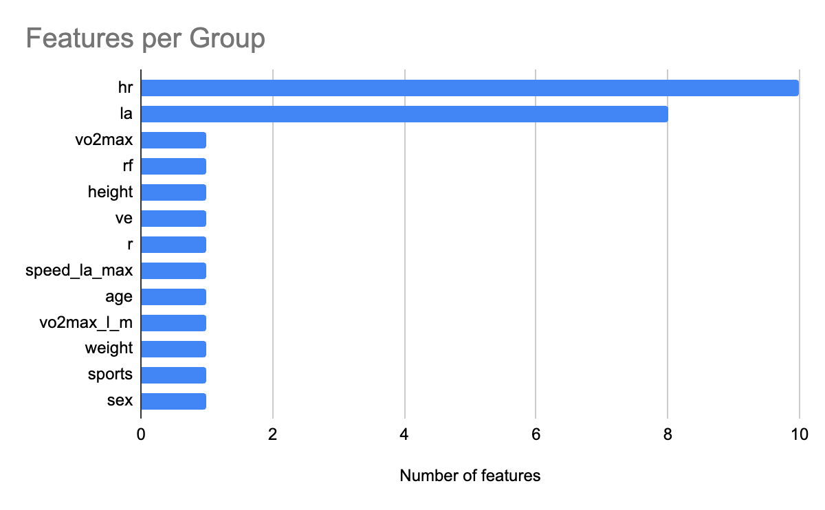
To interpret the XGBoost model, we applied SHAP to quantify the relative contribution of each feature. Figure 6 shows the feature count for each group. We grouped heart rate features and lactic acid levels related features into groups hr and la respectively. Figure 7 shows the relative contribution of each of the feature groups towards AeT prediction. The analysis revealed that heart rate (HR) features dominated model predictions, accounting for 59.2% of total feature importance, followed by lactate (LA) variables contributing 29.5%. Together, these two groups explain nearly 90% of the predictive signal, underscoring the central role of cardiovascular and metabolic responses in determining aerobic and anaerobic thresholds. Secondary contributors included maximal oxygen uptake (VO₂max, 1.9%), respiratory frequency (RF, 1.6%), and anthropometric features such as height (1.4%) and weight (0.8%). Demographic factors such as age, sex, and sport type contributed minimally (<1%), suggesting that individual physiological responses were far more influential than anthropometric and demographic characteristics in predicting performance thresholds.

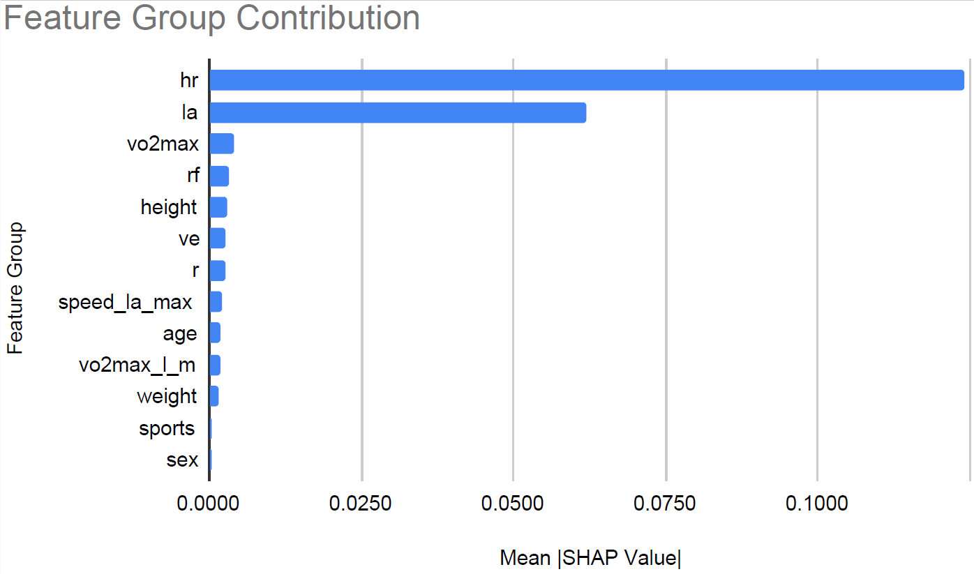
In summary, XGBoost emerged as the best-performing and most physiologically interpretable model, achieving strong predictive accuracy, statistically supported improvements over Random Forest, and biologically consistent feature importance patterns that align with known determinants of aerobic and anaerobic fitness. However, LightGBM and especially ExtraTrees are equally good alternatives especially when compute power and training time are of concern. 

Results for Anaerobic Threshold 

As shown in Table 8, the four hypertuned ensemble models—Random Forest, Extra Trees, XGBoost, and LightGBM—achieved strong performance in both cross-validation and bootstrap testing. The optimal parameters of tuned models are included in Table 9 as well. Their predictive accuracy for AnT surpassed that observed for AeT, with consistently higher R² values and lower error magnitudes.

Across models, R²_test values on the test set ranged from 0.850 to 0.923, indicating strong predictive capability. XGBoost achieved the best overall performance, with R²_test = 0.923 (±0.076), MAE_test = 0.038 (±0.013), and MAPE_test = 2.57% (±0.91%), followed closely by Extra Trees (R²_test = 0.920 ± 0.069, MAPE_test = 2.84% ± 0.88%). Random Forest also demonstrated strong generalization (R²_test = 0.890 ± 0.100), while LightGBM underperformed slightly relative to the others (R²_test = 0.850 ± 0.112) suggesting greater sensitivity to parameter stochasticity and sample variability.

Among them, XGBoost achieved the strongest overall performance, yielding R²_train = 0.911 (±0.055) in cross-validation and R²_test = 0.923 (±0.076) on the bootstrap test set, with the lowest error rates (MAE_test = 0.038 (± 0.013); MAPE_test = 2.57 (± 0.91%)). This is seen for all models including Extra Trees (R²_test = 0.920 ±0.069 and R²_train = 0.902 ± 0.0785). Random Forest also showed robust generalization (R²_test = 0.890 ± 0.100 and R²_train = 0.887 ± 0.0645) though with marginally higher errors (MAPE_test ≈ 3.15%). LightGBM (R²_test = 0.850 ± 0.112 and R²_train = 0.856 ± 0.1075) underperformed slightly relative to the other ensemble methods (MAPE_test ≈ 3.62%).

The consistent alignment of cross-validation and bootstrap test scores across all models suggests minimal overfitting and stable generalization. Overall, gradient boosting–based methods (XGBoost and LightGBM) marginally outperformed bagging-based methods (Random Forest and Extra Trees), likely due to their finer control of bias–variance trade-offs via learning rate and subsampling parameters.

Model Name	Hypertuned Parameter Values	Dataset	R2	MAE	MAPE
Random Forest	max_features: 27, min_samples_split: 5, n_estimators: 300	CV Train	0.887 (± 0.0645)	0.052 (± 0.0145)	3.25% (± 1.05%)
		Bootstrap Test	0.890 (± 0.100)	0.047 (± 0.015)	3.15% (± 1.03%)
Extra Trees	max_features: 28, min_samples_split: 5, n_estimators: 300	CV Train	0.902 (± 0.0785)	0.048 (± 0.015)	2.94% (± 1.06%)
		Bootstrap Test	0.920 (± 0.069)	0.042 (± 0.013)	2.84% (± 0.88%)
XGBoost	colsample_bynode: 0.9, learning_rate: 0.03, n_estimators: 500, subsample: 0.6	CV Train	0.911 (± 0.0545)	0.046 (± 0.012)	2.87% (± 0.76%)
		Bootstrap Test	0.923 (± 0.076)	0.038 (± 0.013)	2.57% (± 0.91%)
Light GBM	colsample_bynode: 0.6, learning_rate: 0.02, n_estimators: 500, subsample: 0.6	CV Train	0.856 (± 0.1075)	0.057 (± 0.0155)	3.53% (± 0.83%)
		Bootstrap Test	0.850 (± 0.112)	0.054 (± 0.019)	3.62% (± 1.34%)

Table 9 compares the predictive performance of the ensemble models developed in this study with those reported by Tomaszewski et al. (2024) for estimating the anaerobic threshold (AnT). Overall, the models in the present study demonstrated improved generalization performance, as reflected by higher R²_test values across all algorithms.

Specifically, the Random Forest model achieved a test R²_test= 0.890 slightly exceeding the R²_test= 0.789 reported by Tomaszewski et al., despite a lower training R²_train (0.887 vs. 0.970), suggesting reduced overfitting and more stable generalization. Similarly, XGBoost showed the highest test performance among all models, with R²_test= 0.923 compared to R²_test = 0.716 in Tomaszewski et al., indicating substantial improvement in predictive accuracy. The LightGBM model also demonstrated comparable generalization, with R²_test= 0.850 versus 0.803 in Tomaszewski et al.

Taken together, these results indicate that while the models in this study exhibit slightly lower training accuracy, they generalize better to unseen data, likely due to improved regularization, cross-validation, and bootstrap-based evaluation strategies.

	Tomaszewski		Our Models
Algorithm	R² Train	R² Test	R² Train	R² Test
Random Forest	0.970	0.789	0.887	0.890
XGBoost	0.995	0.716	0.911	0.923
Light GBM	0.965	0.803	0.856	0.850

To assess whether the observed differences in predictive performance among the ensemble models were statistically significant, we applied the Nadeau–Bengio corrected t-test. This approach accounts for dependencies introduced by repeated k-fold cross-validation, mitigating the risk of optimistic bias or results driven by chance splits. By employing repeated cross-validation, we further reduced the influence of random partitioning effects and ensured more stable estimates of model performance.

The statistical comparison (Table 10) revealed that, for AnT prediction, XGBoost significantly outperformed Random Forest (p = 0.0338), demonstrating a small but consistent advantage (ΔR² = 0.016). All other pairwise comparisons, including those between Extra Trees, LightGBM, and XGBoost, did not show statistically significant differences. These findings indicate that while all ensemble models achieved comparable predictive performance, XGBoost provided a modest yet statistically supported improvement over Random Forest in modeling the anaerobic threshold.

Model	Model	Better Model	ΔR²	P-value	Significant (p<0.05)
RF	ET	ET	0.0154	0.1549	No
RF	XGBoost	XGBoost	0.016	0.0338	Yes
RF	LGBM	RF	0.0332	0.2763	No
ET	XGBoost	XGBoost	0.0006	0.9275	No
ET	LGBM	ET	0.0486	0.0791	No
XGBoost	LGBM	XGBoost	0.0492	0.1042	No

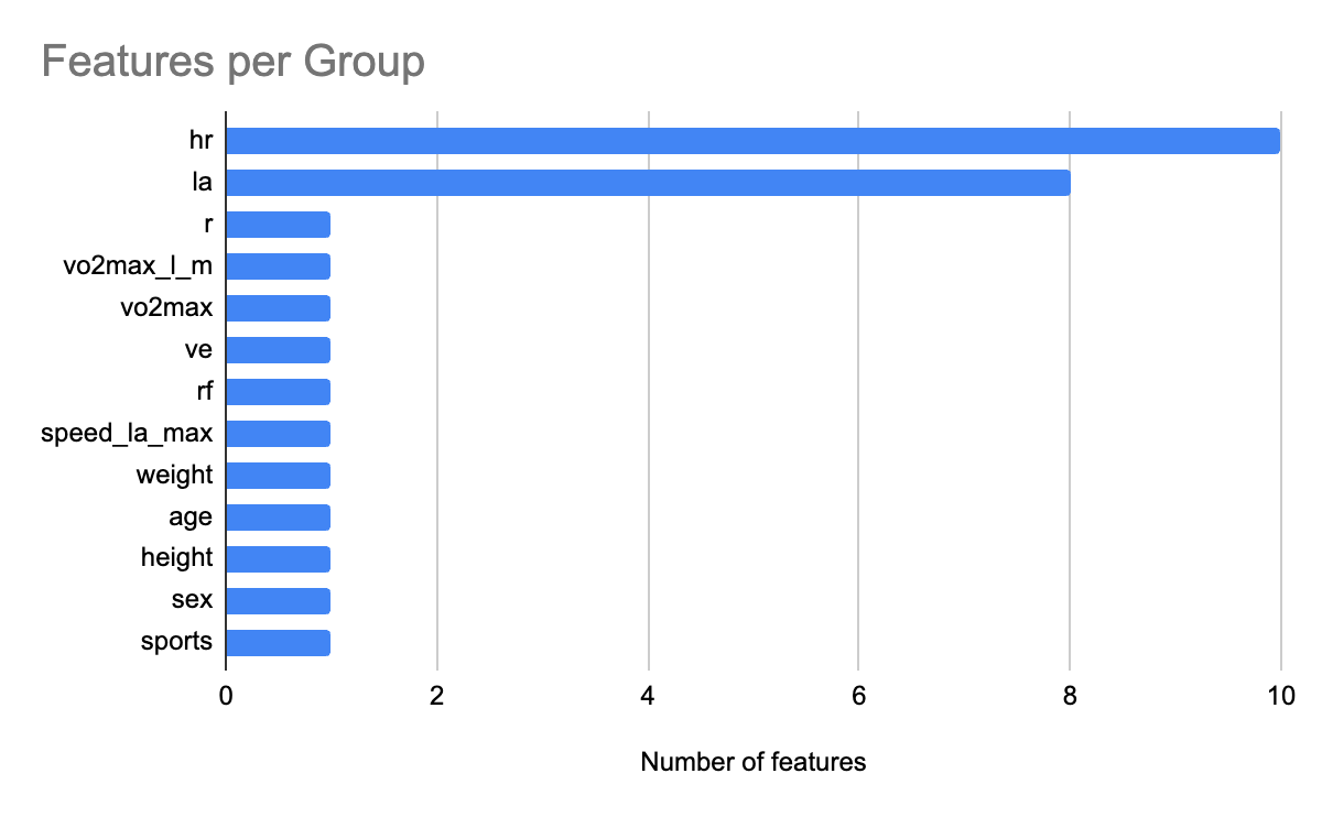
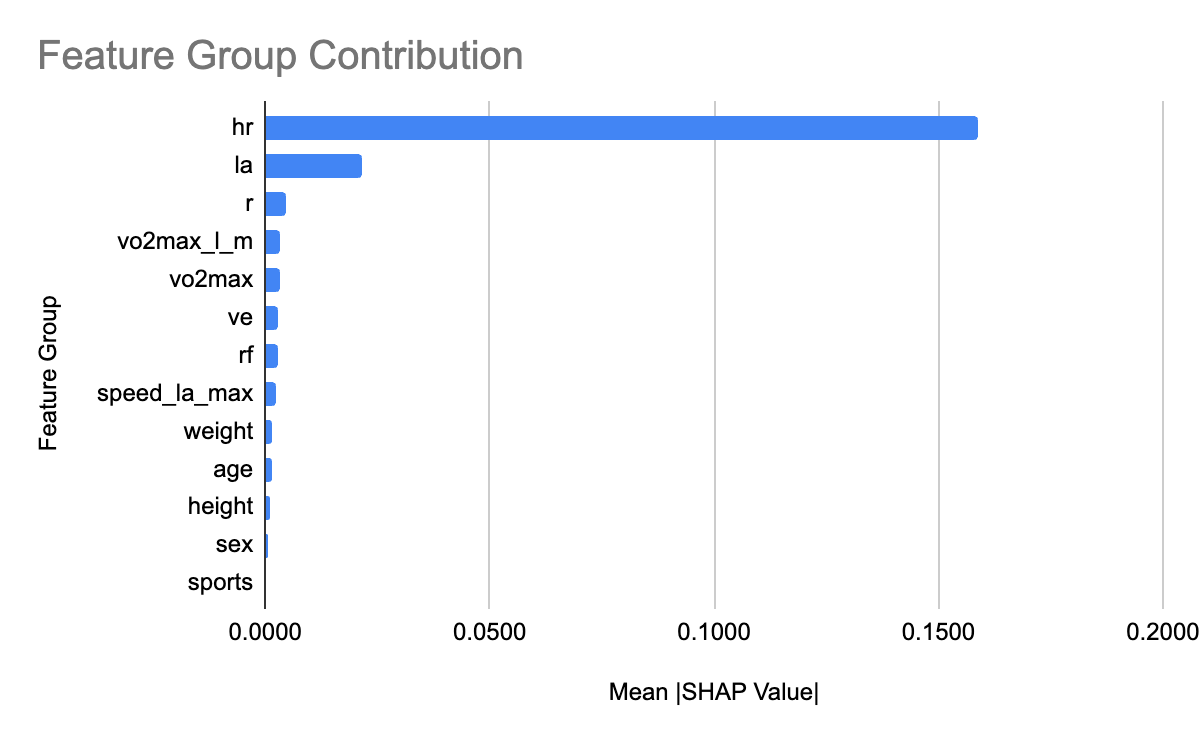
We leverage SHAP analysis to quantify the relative contribution of each feature towards AnT prediction. Figure 8 shows the feature count for each group. Similar to AeT, we grouped heart rate features together into the group hr and grouped lactic acid levels related features into a group called la for AnT feature importance analysis. Figure 9 shows the relative contribution of each of the feature groups towards AnT prediction. We find that heart rate related features were by far the dominant predictors of the AnT, accounting for 77.8% of the total model attribution. Lactic acid (La) features contributed 10.5%, indicating their secondary but complementary role in capturing metabolic stress responses. This strong influence reflects the physiological dependence of AnT on cardiovascular response dynamics across incremental workloads. 

All other feature groups such as respiratory frequency (rf), oxygen uptake variables (VO₂max and VO₂max_l_m), ventilation (Ve), and body composition indicators (weight, height, age) had relatively minor contributions, each below 3%. These lower but non-negligible effects suggest that while AnT is primarily governed by cardiovascular and metabolic variables, anthropometric and respiratory characteristics provide fine-grained adjustments that improve prediction accuracy.

Overall, the SHAP dependency patterns align with established physiological theory, confirming that heart rate progression and lactate accumulation jointly encapsulate the key determinants of anaerobic threshold performance.

Discussion

Among the four hypertuned ensemble models, Random Forest, Extra Trees, XGBoost, and LightGBM, XGBoost consistently achieved the highest predictive performance for both AeT and AnT. For AeT, XGBoost not only demonstrated superior predictive accuracy but also maintained better confidence intervals and significant improvement over Random Forest according to statistical testing. Extra Trees emerged as a strong alternative, particularly advantageous when computational efficiency is a concern. LightGBM performed competitively for AeT but showed reduced stability and accuracy for AnT, whereas Random Forest consistently underperformed across both thresholds. We found the confidence intervals consistent over train and test datasets for each of the models suggesting good model generalization. While the CI are not necessarily tight, possibly because of the small size of the dataset, they show consistency across models as well as metrics if we normalize the CI interval by the mean of the respective metrics.

SHAP analysis provided interpretability into the model mechanisms. In order to obtain more meaningful insights, we applied domain-driven grouping of related variables grouping heart related features into group hr and lactic acid related features into the group la. The contribution of a group is the sum of the contribution of individual features in the group. We chose conceptual grouping to enhance interpretability. Heart rate (HR) and lactate (La) features dominated model predictions, collectively contributing nearly 90% of the total SHAP importance, underscoring their physiological relevance as key determinants of metabolic transition points. Variables related to respiratory function (like VO₂max) contributed modestly, while anthropometric and demographic features (e.g., age, sex, height, weight) had minimal predictive influence. This aligns with established physiological theory that threshold responses are largely driven by cardiovascular and metabolic factors rather than physical characteristics. 

Compared with prior work by Tomaszewski et al. (2024), which employed similar ensemble approaches on the same dataset, our models demonstrated improved generalization performance, particularly in R²_test scores. This improvement likely stems from our robust training design incorporating repeated cross-validation and statistical control for overfitting. Collectively, these findings highlight that well-regularized ensemble learning can outperform manually estimated thresholds and prior benchmark models, enhancing the reliability and scalability of ML-based threshold estimation.

Despite these advances, there are limitations that should be acknowledged. The dataset, derived from Tomaszewski et al. (2024), included 183 amateur athletes, likely representing a homogeneous regional cohort. This limits the generalizability of results to elite, recreational, or untrained populations, and likely to other geographical areas and ethnic groups. The cross-sectional design also precludes insight into longitudinal changes in threshold dynamics or adaptations to training interventions. Furthermore, external validation on independent cohorts was not feasible, which remains a critical step for confirming robustness. Finally, the assumption of uniformity in test procedures and participant preparation may not fully account for individual variability inherent in physiological measurements.

Individualized predictions of aerobic and anaerobic thresholds have strong practical value for both athletes and coaches, enabling the precise planning of training intensities, monitoring of effort in real time, and optimization of performance strategies. By anchoring training zones to personal physiological thresholds rather than population-based formulas, athletes can target specific goals while minimizing fatigue and overtraining risk. During training and competition, real-time monitoring of heart rate can enable intelligent pacing (e.g, for marathon runners) and energy management (e.g. for player substitutions in football). Over time, repeated threshold estimation provides a quantitative measure of fitness progression, recovery, and adaptation, helping refine training cycles. Beyond performance, individualized AeT and AnT estimates have broader applications in rehabilitation, return-to-sport protocols, and digital coaching platforms that integrate physiological feedback for adaptive training recommendations. These personalized models help bridge laboratory assessment and real-world training with an evidence-based framework for optimizing endurance performance and athlete health.

Conclusion

This study developed and evaluated machine learning models to predict aerobic (AeT) and anaerobic (AnT) thresholds from physiological and performance data, providing an interpretable, data-driven framework for performance assessment. Using a balanced ensemble-based approach, combining bagging (Random Forest, Extra Trees) and boosting (XGBoost, LightGBM) methods, we applied rigorous model optimization and validation, including repeated cross-validation, bootstrap confidence intervals, and the Nadeau–Bengio corrected t-test to ensure statistical robustness and minimize overfitting.

Across both AeT and AnT predictions, all four ensemble models demonstrated strong performance, with XGBoost and Extra Trees exhibiting the most consistent accuracy and stability across both AeT and AnT predictions. While XGBoost achieved the highest mean predictive performance, statistical testing indicated that differences among XGBoost, Extra Trees and LightGBM models were not always significant, underscoring the overall reliability of ensemble-based approaches. 

Compared with prior work (Tomaszewski et al., 2024), our models achieved improved predictive accuracy and demonstrated stronger generalization to unseen data, achieved through more rigorous validation and explainability analyses. These findings support the use of ensemble machine learning as a complementary, potentially more scalable approach to traditional manual threshold determination. These results support the growing role of data-driven approaches in exercise physiology, enabling individualized performance assessment and real-time training optimization.

SHAP-based explainability analysis revealed that heart rate–derived features and blood lactate responses were the dominant predictors for both thresholds, highlighting the central role of cardiovascular and metabolic dynamics. In contrast, demographic and anthropometric features (e.g., sex, age, height, weight) contributed minimally, suggesting that physiological responses are more predictive of threshold variation than static individual characteristics. While we used domain-driven grouping of related variables, experimenting with SHAP interaction values or correlation-clustered aggregation to gain further insights can be a future research item.

Nonetheless, this study has limitations. The dataset was relatively small and homogeneous, comprising trained amateur athletes from a single cohort, which constrains generalizability. The analysis was cross-sectional and did not capture longitudinal training adaptations or seasonal variations. Furthermore, the models have not yet been externally validated on independent datasets.

Future research should focus on validating these models across diverse populations, expanding to include recreational or untrained individuals, and integrating multimodal sensor data (e.g., wearable metrics) for real-time monitoring. Longitudinal studies are also warranted to examine how AeT and AnT evolve over time and with different training interventions. Collectively, these directions will strengthen the robustness, applicability, and translational value of machine learning–based threshold prediction in sports physiology.

References

1. M. Tomaszewski, A. Lukanova-Jakubowska, E. Majorczyk, & Ł. Dzierżanowski. (2024). From data to decision: Machine learning determination of aerobic and anaerobic thresholds in athletes. PLOS ONE, 19(8), e0309427. [↩]
2. J. Brownlee. (2021). XGBoost with Python: Gradient Boosted Trees with XGBoost and Scikit-Learn. Machine Learning Mastery Press. [↩] [↩]
3. J. Esteve-Lanao, A. F. San Juan, C. P. Earnest, C. Foster, & A. Lucia. (2007). How do endurance runners actually train? Relationship with competition performance. Medicine & Science in Sports & Exercise, 39(2), 303–311. [↩] [↩]
4. A. W. Midgley, L. R. McNaughton, & A. M. Jones. (2007). Training to enhance the physiological determinants of long-distance running performance. Sports Medicine, 37(10), 857–880. [↩]
5. R. K. Binder, M. Wonisch, U. Corra, A. Cohen-Solal, L. Vanhees, H. Saner, & J. P. Schmid. (2008). Methodological approach to the first and second lactate threshold in incremental cardiopulmonary exercise testing. European Journal of Cardiovascular Prevention & Rehabilitation, 15, 726–734. [↩]
6. V. L. Billat. (2001). Interval training for performance: A scientific and empirical practice. Sports Medicine, 31(1), 13–31. [↩]
7. American College of Sports Medicine. (2014). ACSM’s guidelines for exercise testing and prescription (9th ed.). Wolters Kluwer/Lippincott Williams & Wilkins Health. [↩]
8. H. Traninger, M. Haidinger, A. H. Zemljic-Harpf, & H. H. Harpf. (2020). Personalized determination of target training heart rates for all ages, including patients with heart disease. The FASEB Journal, 34, 1–1. [↩]
9. A. Marx, J. Porcari, S. Doberstein, B. Arney, S. Bramwell, & C. Foster. (2018). The accuracy of heart rate-based zone training using predicted versus measured maximal heart rate. International Journal of Research in Exercise Physiology, 14, 21–28. [↩] [↩] [↩]
10. P. Hofmann, S. P. von Duvillard, F. J. Seibert, R. Pokan, M. Wonisch, L. M. Lemura, & J. P. Schmid. (2001). HRmax target heart rate is dependent on heart rate performance curve deflection. Medicine & Science in Sports & Exercise, 33, 1726–1731. https://pubmed.ncbi.nlm.nih.gov/11581558 [↩]
11. A. M. Jones, & H. Carter. (2000). The effect of endurance training on parameters of aerobic fitness. Sports Medicine, 29(6), 373–386. [↩]
12. P. Razanskas, A. Verikas, C. Olsson, & P.-A. Viberg. (2015). Predicting blood lactate concentration and oxygen uptake from sEMG data during fatiguing cycling exercise. Sensors, 15(8), 20480–20500. [↩] [↩]
13. S. Kobayashi, T. Yamada, & H. Nakamura. (2023). Prediction of blood lactate concentrations after cardiac surgery using machine learning and deep learning approaches. Frontiers in Cardiovascular Medicine, 10, 10543087. [↩]
14. K. Sughimoto, S. Okada, & Y. Nakajima. (2023). Machine learning predicts blood lactate levels in children after cardiac surgery in paediatric ICU. Cardiology in the Young, 33(8), 1523–1531. https://doi.org/10.1017/S1047951123000362 [↩]
15. J. Vos, S. Rahman, & P. Gupta. (2022). Ensemble machine learning model trained on a synthesized dataset generalizes well for stress prediction using wearable devices. arXiv preprint arXiv:2209.15146. [↩] [↩]
16. S. M. Lundberg, & S.-I. Lee. (2017). A unified approach to interpreting model predictions. Advances in Neural Information Processing Systems (NeurIPS), 30. [↩] [↩]
17. S. Villafaina, D. Collado-Mateo, J. P. Fuentes-García, R. de la Vega, N. Gusi, & V. J. Clemente-Suárez. (2023). Identification of athleticism and sports profiles through machine learning applied to heart rate variability. Sensors, 23(18), 7804. [↩]
18. M. Saar-Tsechansky, & F. Provost. (2007). Handling missing values when applying classification models. Journal of Machine Learning Research, 8, 1625–1657. [↩]
19. J. C. Jakobsen, C. Gluud, J. Wetterslev, & P. Winkel. (2017). When and how should multiple imputation be used for handling missing data in randomized clinical trials—a practical guide with flowcharts. BMC Medical Research Methodology, 17(1), 162. [↩]
20. F. Pedregosa, G. Varoquaux, A. Gramfort, V. Michel, B. Thirion, O. Grisel, … É. Duchesnay. (2011). Scikit-learn: Machine learning in Python. Journal of Machine Learning Research, 12, 2825–2830. [↩]
21. M. Falbriard, F. Meyer, B. Mariani, G. P. Millet, & K. Aminian. (2020). Drift-free foot orientation estimation in running using wearable IMU. Frontiers in Bioengineering and Biotechnology, 8, 65. [↩]
22. E. Mulder, C. van der Meijden, J. de Korte, & P. F. F. Wijn. (2019). Exercise-induced changes in compensatory reserve and heart-rate complexity. Frontiers in Physiology, 10, 1471. [↩]
23. C. Siebenmann, P. Rasmussen, & C. Lundby. (2020). Effects of baseline heart rate at sea level on cardiac responses to high-altitude exposure. European Heart Journal, 41(10), 1035–1043. [↩]
24. G. S. Zavorsky, K. A. Tomko, & J. M. Smoliga. (2012). Decline in resting heart rate with endurance training: Meta-analysis of 112 studies. European Journal of Applied Physiology, 112(9), 3479–3491. [↩]
25. S. Kobayashi, T. Yamada, & H. Nakamura. (2023). Prediction of blood lactate concentrations after cardiac surgery using machine learning and deep learning approaches. Frontiers in Cardiovascular Medicine, 10, 10543087. https://doi.org/10.3389/fcvm.2023.10543087 [↩]
26. K. Sughimoto, S. Okada, & Y. Nakajima. (2023). Machine learning predicts blood lactate levels in children after cardiac surgery in pediatric ICU. Cardiology in the Young, 33(8), 1523–1531. https://doi.org/10.1017/S1047951123000362 [↩]
27. L. Breiman. (2001). Random forests. Machine Learning, 45(1), 5–32. [↩]
28. P. Geurts, D. Ernst, & L. Wehenkel. (2006). Extremely randomized trees. Machine Learning, 63(1), 3–42. [↩]
29. T. Chen, & C. Guestrin. (2016). XGBoost: A scalable tree boosting system. Proceedings of the 22nd ACM SIGKDD International Conference on Knowledge Discovery and Data Mining, 785–794. [↩] [↩] [↩]
30. G. Ke, Q. Meng, T. Finley, T. Wang, W. Chen, W. Ma, & T.-Y. Liu. (2017). LightGBM: A highly efficient gradient boosting decision tree. Advances in Neural Information Processing Systems, 30, 3149–3157. [↩] [↩] [↩] [↩]
31. M. Kuhn, & K. Johnson. (2013). Applied predictive modeling. Springer. [↩] [↩] [↩]
32. A. Géron. (2022). Hands-On Machine Learning with Scikit-Learn, Keras, and TensorFlow (3rd ed.). O’Reilly Media. [↩]
33. L. Prokhorenkova, G. Gusev, A. Vorobev, A. V. Dorogush, & A. Gulin. (2018). CatBoost: Unbiased boosting with categorical features. Advances in Neural Information Processing Systems (NeurIPS), 31. [↩] [↩]
34. T. Zhao, Y. Zeng, & C. Zheng. (2020). Empirical evaluation of hyperparameter optimization for gradient boosting decision trees. Applied Sciences, 10(19), 6790. [↩]
35. G. Louppe. (2014). Understanding Random Forests: From theory to practice. arXiv preprint arXiv:1407.7502. [↩] [↩] [↩]
36. J. Demšar. (2006). Statistical comparisons of classifiers over multiple data sets. Journal of Machine Learning Research, 7, 1–30. [↩] [↩]
37. A. Labach, H. Salehinejad, & S. Valaee. (2022). Interpretation of deep learning models for EEG-based emotion recognition: Domain-informed SHAP grouping for physiological interpretability. Frontiers in Neuroscience, 16, 834517. [↩]