Disentangling New Physics in Single Resonant Top Quarks

Krish Wu, Brandon Sun, Nitish Polishetty, Justin Kline, Max Fieg & Daniel Whiteson

December 10, 2025

Abstract

Collisions of particles at the energy frontier can reveal new particles and forces via localized excesses in invariant mass distributions. However, the initial observation may be consistent with a large variety of theoretical models, especially in sectors with new top quark partners, which feature a rich set of possible underlying interactions. We explore the power of the Large Hadron Collider dataset to distinguish between models of the singly produced heavy top-like quark which interacts with the Standard Model through an electromagnetic form factor. We study the heavy top decay to a top quark and a virtual photon which produces a pair of fermions, propose a technique to disentangle the models, and calculate the expected statistical significance to distinguish between various hypotheses.

Introduction

Many theories of new physics predict striking phenomena observable in high-energy collisions. In some cases, the potential experimental signatures are consistent with several distinct models of new particles or interactions, and disentangling them can be quite difficult¹^‘². The discovery of the Higgs boson³^‘⁴, for example, has been followed by precision measurements of its properties⁵^‘⁶ to determine whether it is the garden variety boson of the Standard Model, or something more exotic, a question whose answer is still being resolved. In the event that a discovery of a new particle is made, whether anticipated or not⁷^‘⁸, it can be expected to spark a similar effort to distinguish potential theoretical explanations. The top quark sector has a rich set of models predicting new heavy partners, with multiple experimental signatures. In some cases, as in the scenario studied here, the nature of the production and decay can be quite similar across theoretical models, even if the form of the interactions is quite different.

Recently, we proposed⁹ the study of single production of a heavy vector-like quark T, which for high T masses features higher cross sections than pair production, and can include decays such as $T \rightarrow t\gamma$ ¹⁰, which can dominate in some scenarios¹¹ over the more commonly studied T $\rightarrow$ Wb,Zt,Ht. Searches by the Large Hadron Collider (LHC) collaboration have primarily studied T decays featuring heavy bosons, $T \rightarrow Wb,Zt,Ht$ ¹²^‘¹³^‘¹⁴^‘¹⁵^‘¹⁶^‘¹⁷^‘¹⁸^‘¹⁹^‘²⁰. Studies of T $\rightarrow \gamma t$ have received less attention,and primarily focused on pair production of the new heavy fermion¹¹. ATLAS explored the $t\gamma$ final state²¹, but did not search for a $t\gamma$ resonance.

In this paper, we revisit single production of heavy vector-like quarks that interact through the photon via electromagnetic (EM) form factor operators. We study again the single production mode and focus on the decay $T \rightarrow t\gamma$ $\rightarrow$ $tf^{+}f^{-}$ , where the photon is off-shell and converts to a pair of fermions ( $f^{+}f^{-}$ ). This mode is shared by the dimension-5 and dimension-6 EM form factor operators, which allows us to explore several distinct theoretical models, predict T production at the LHC, and examine the power of the LHC dataset to distinguish between these models.

The paper is organized as follows. The first section describes the theoretical models of the heavy top partner and the experimental sensitivity to the various models. The following sections discuss the results, and the final section describes the methods in detail.

Results

Models

Vector-like top partners²² are typically found in models that alleviate the hierarchy problem and are less constrained than a 4th generation of quarks with chiral couplings²³^‘²⁴^‘²⁵. These particles can be found in more complete models such as Little Higgs models²⁶, supersymmetric theories, composite Higgs models²⁷ or in scenarios where the right-handed top quark is composite and T is an excited state²⁸^‘²⁹. However, the compatibility of these motivations and the model we study are dependent on the details of the underlying theory.

**Figure 1 |** Feynman diagram describing the single production of a heavy vector-like fermionic top partner $T$ which decays to a top quark ( $t$ ) and a photon ( $\gamma$ ), which then decays to a pair of charged leptons ( $\ell^+\ell^-$ )

In this work, we consider a class of models where a vector-like quark $T$ , which has the same quantum numbers as a right-handed up-type quark, and can interact with the SM up-type quarks through electromagnetic form factor operators up to dimension-6. In particular, we consider an interaction taking the form of a dimension-5 magnetic and electric dipole moment (MDM, EDM), and the dimension-6 anapole and charge radius (CR) operators. The Lagrangians that govern these interactions can be written as the following:

(1) $\begin{equation*}\mathcal{L}{\rm MDM} = \mu_i\, \bar{T}\,\sigma^{\mu \nu}\, u{R,i}\, F_{\mu\nu}\end{equation*}$

(2) $\begin{equation*}\mathcal{L}{\rm EDM} = d_i\, \bar{T}\,\sigma^{\mu \nu}\gamma^{5}\, u{R,i}\, F_{\mu\nu}\end{equation*}$

(3) $\begin{equation*}\mathcal{L}{\rm Anapole} = a_i\, \bar{T}\,\gamma^{\mu}\gamma^{5}\, u{R,i}\, \partial^{\nu} F_{\mu\nu}\end{equation*}$

(4) $\begin{equation*}\mathcal{L}{\rm CR} = b_i\, \bar{T}\,\gamma^{\mu}\, u{R,i}\, \partial^{\nu} F_{\mu\nu}\end{equation*}$

where $u_{R,i}$ is a right-handed up-type quark, $\mu_i,d_i,a_i,b_i$ are dimensionful couplings of $T$ to a quark with flavor $i$ .

Vector-like top quarks can be found, for example, in Little Higgs models²⁶ or in composite top quark models²⁸^‘³⁰^‘³¹. This effective interaction can arise in a UV model where heavy particles with electroweak charges have been integrated out¹¹ or where the top quark is composite, and these interactions mediate radiative transitions with the excited state T³². The dimension-6 operators are studied less frequently in the literature, but we nevertheless wish to assess their signatures as they could generically arise through analogous mechanisms. The physics responsible for these interactions is at or above the TeV-scale. For $m_T \approx$ O(TeV), the new state can only be directly produced at the LHC, and may be searched for with jet + photon signatures³³ for the EDM and MDM operators, while the higher dimensional operators could be searched for with trijet signatures³⁴ or dilepton + jet. Some of these interactions can also be searched for indirectly, in particular the anapole and EDM operators lead to parity violation which can be indirectly tested in atomic systems³⁵. The dimension-5 operators induce a T $\rightarrow$ $t\gamma$ decay, and while the partial decay width of this channel for the dimension-6 operators is zero for an on-shell photon, the offshell photon decaying to a pair of fermions has nonzero width. Thus, the four models produce $tf^{+}f^{-}$ , allowing a direct comparison of the kinematics in the same final states.

Z + b\bar{b} + \gamma — **Table 1 |** Expected yields ( $N$ ) in 300 fb $^{-1}$ of LHC $pp$ collisions at $\sqrt{s}=13$ TeV for several background processes. Cross sections for backgrounds are at NLO in QCD³⁶.

Process	N
$t\bar{t}\gamma$	2730
$Z + b\bar{b} + \gamma$	681
$W + b\bar{b} + \gamma$	256
$t \bar{b}\gamma + \bar{t}b\gamma$	21

Experimental Sensitivity

The models described above include interactions which can generate a final state with a top quark and a pair of opposite-sign charged leptons; see Figure 1. We estimate the sensitivity of the LHC dataset to these hypothetical signals using samples of simulated pp collisions at $\sqrt{s}=13$ TeV with an integrated luminosity of 300 fb $^{-1}$ . Generation of simulated signal and background events as well as the recontruction strategy are described below.

The dominant backgrounds are the production of top quark pairs with an additional pair of leptons ( $t\bar{t}\ell^+\ell^-$ ), or the production of a single top quark in association with a b quark ( $\bar{t}b\ell^+\ell^-$ ) and a pair of leptons. Additional backgrounds are due to production of a heavy vector boson (W or Z bosons) in association with b quarks and a pair of leptons, $W b \bar{b} \ell^+ \ell^-$ or $Zb \bar{b} \ell^+ \ell^-$ .Contribution from QCD multi-jet production is suppressed by the lepton requirement and the minimum $m_T$ , and are non-zero but sub-dominant and are neglected here. Distributions of the expected reconstructed T quark masses and the photon transverse momentum for the background and signal processes are shown in Figure 3 and the expected background yields in 300 fb $^{-1}$ are shown in Table 1.

Statistical Analysis

Expected limits on the single T production cross section are calculated at 95% confidence level (CL) using a profile likelihood ratio³⁷ with the CLs technique³⁸^‘³⁹). We use the pyhf⁴⁰^‘⁴¹ package with a binned distribution in heavy quark reconstructed mass, where bins without simulated background events have been merged into adjacent bins. The background is assumed to have a 50% relative systematic uncertainty. Limits on the signal cross section as a function of the T quark mass are shown in Figure 4.

**Figure 2 |** Distribution of the reconstructed heavy top ( $T$ ) quark candidate mass in simulated events with $m_T=1000$ (solid) or 2000 (dashed) GeV, for MDM (top) and Anapole (bottom) models for each of the three reconstruction strategies (see Fig 7). The overall normalization is arbitrary, but the relative density of reconstruction modes reflects the different top quark $p_\textrm{T}$ predicted by the two models in the $T\rightarrow t\gamma$ decay.

Distinguishing between the various models using only the reconstructed heavy quark invariant mass would be challenging given the similarity in the mass distributions. But there is more information present in the events that can reveal the nature of the underlying interaction. The dimension-6 operators have an additional dependence on the virtual photon’s momenta in the Lagrangian, as shown in equations 1–4, and thus will display a strong difference in the kinematic distribution in the final state leptons, as is seen in the distribution of reconstructed photon momentum in the bottom panel of Figure 3. Distributions for MDM and EDM models are very similar, as those from the CR and Anapole models; only CR and EDM are shown, for two choices of $m_T$ .

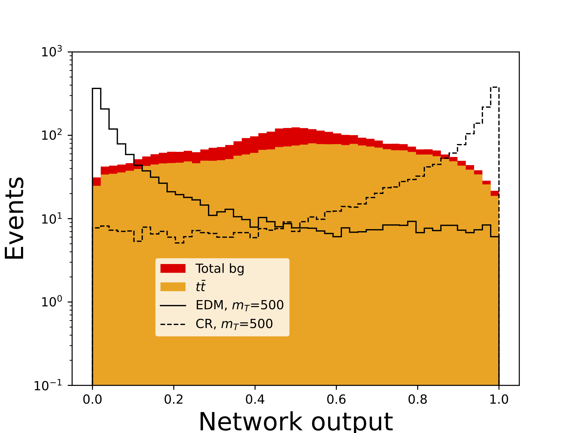
To capture the full discrimination information available, we train a neural network (NN) to distinguish between the heavy quark models. The network inputs are the four vectors of the reconstructed top quark and photon. Three hidden layers are used, consisting of 100 nodes, 80 nodes, and 20 nodes respectively, each with a ReLU activation. The final layer has a single sigmoid neuron. In training, the dimension-5 models were given label 0 and the dimension-6 models label of 1. The loss function is binary cross entropy and mini-batch training with batch sizes of 10 was used, along with the Adam optimizer. Each sample had approximately 100,000 events, and an independent network was trained for each of the candidate heavy quark masses considered. One quarter of the data were reserved for testing, and training continued until peformance plateaued on the testing sample, to avoid overfitting.

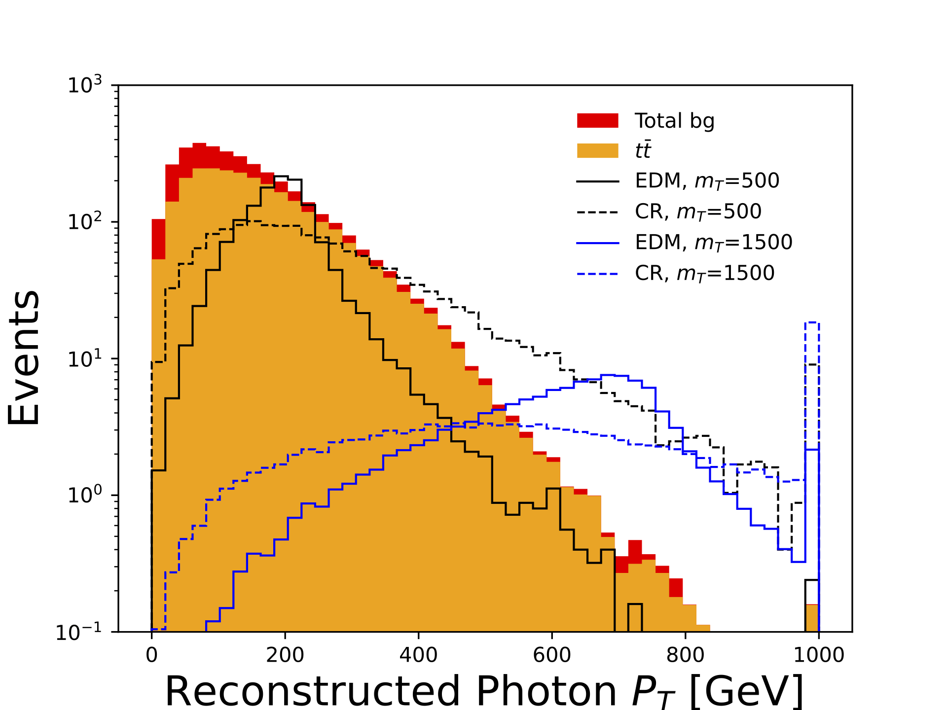**Figure 3 |** Distribution of reconstructed heavy quark invariant mass (top) or photon $p_\textrm{T}$ in simulated signal and background samples, normalized to an integrated luminosity of 300 fb $^{-1}$ . The last bin shows overflow. The signal cross section is set to the expected limit at 95% CL.

The output of the network and its discrimination power is shown in Figure 5, showing significantly more discrimination power than the top or photon transverse momenta individually.

To assess the power of the dataset to distiguish between these models, we calculate the likelihood ratio (LR) between the dimension-5 and dimension-6 models using the binned network output to estimate the densities. We calculate the p-value under the dimension-5 scenario of observing the mean LR expected in the dimension-6 scenario as a function of the signal cross section, and vice versa. Results are shown in Figure 6 and indicate that as the heavy quark mass increases, the signal cross section needed to obtain a p-value of less than 0.05 decreases, due to falling background rates. For $m_T \approx$ 1000 GeV, sufficient statistics can be achieved for 300 fb $^{-1}$ , for a cross section greater than about 0.1 fb.

**Figure 4 |** Expected 95% CL upper limits on the production cross section for signal models, as a function of heavy top quark mass.

Discussion

While the various models produce the same list of final state objects and very similar heavy quark mass distributions, the full kinematics of the events allow us to disentangle the dimension-5 and dimension-6 hypotheses. There are additional handles that might help, such as searching for on-shell production of photons, which are expected in dimension-5 models but not in dimension6. The on-shell photon in dimension-5 models also allow for a photon in the initial state, where $\gamma q$ $\rightarrow$ T $\rightarrow$ $t\gamma$ gives a very similar final state and could contribute to the production rate, though the photon parton distribution function (PDF) is more uncertain than quark PDFs. Other experiments and final states can also play an important role. In the event of non-zero mixing between T and uR, electroweak precision observables can be used to constrain mixing parameters⁴²^‘⁴³^‘⁴⁴^‘⁴⁵. Furthermore, flavor changing neutral current processes have been used to constrain vector-like fermions⁴⁶^‘⁴⁷^‘⁴⁸^‘⁴⁹^‘⁵⁰. In addition to direct searches at the LHC, vector-like quarks in the O(100) GeV mass range can be searched for at the Tevatron⁵¹. The studies above demonstrate the possibility of distinguishing between dimension-5 and dimension-6 electromagnetic form factor models, but do not explore whether data could be used to prefer one of the models of equal dimensionality. The kinematics of the production and decay appear to be indistinguishable upon inspection of the distributions and attempts to train a machine learning model.

**Figure 5 |** Distribution of neural network output trained for the $m_T=500$ GeV scenario, shown for simulated signal and background samples normalized to an integrated luminosity of 300 fb $^{-1}$ . The signal cross section is set to the expected limit at 95% CL.
Signal and background efficiency for various thresholds on photon transverse momentum, heavy quark transverse momentum or the neural network output, also for the $m_T=500$ GeV case.

While our methods do not distinguish between operators of the same dimension, it may be possible to differentiate these models by leveraging observables related to angular correlations of the final state particles, which are sensitive to the CP structure of the interaction⁵²^‘⁵³. Theoretically, distinguishing between parity-conserving and parity-violating operators of the same dimension could be achieved using a polarized beam, an option not available at the LHC, but potentially feasible at a future electron⁵⁴ or muon collider⁵⁵. While these models do predict differences in the overall production rate at the LHC, the unknown coupling strength means that an observed rate could be compatible with either scenario.

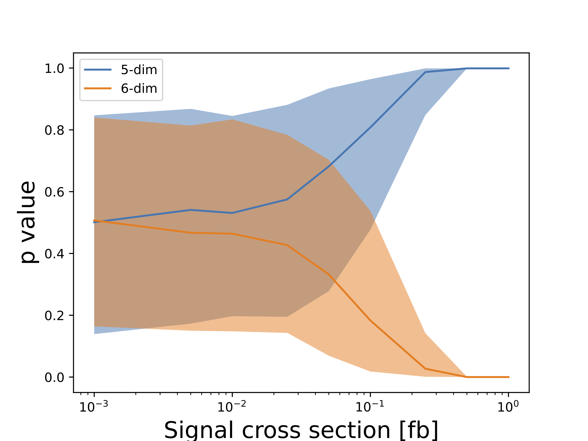
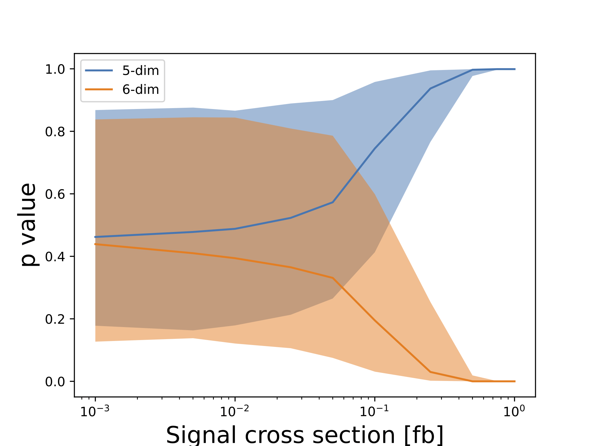
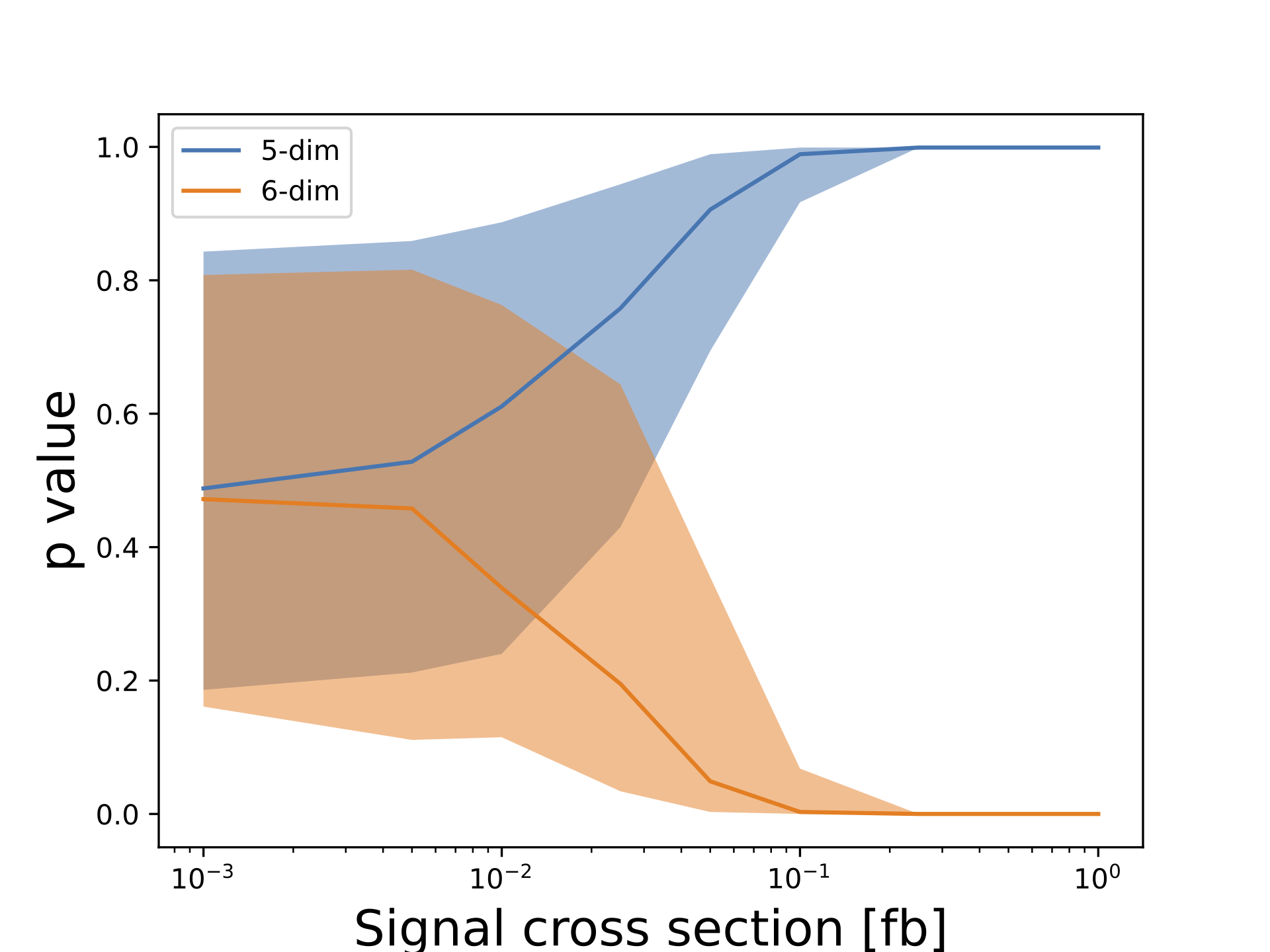
**Figure 6 |** Expected $p$ -values under a dimension-5 hypothesis of observing a neural network output distribution expected from the dimension-6 hypothesis, and vice versa, as a function of the signal production cross section. Shown are the median case (solid line) and an envelope containing 95% of hypothetical similar experiments for the 500, 1000, 1500 and 2000 GeV scenarios (top to bottom).

In conclusion, we present an example of a set of theoretical models which have different underlying mechanisms but would produce similar excesses in reconstructed invariant mass peaks. The theoretical distinctions lead to differences in other kinematic information in the event, which can be exploited in this case to disentangle two categories of models, those with dimension-5 and dimension-6 operators. We train a neural network to capture and summarize these differences. In a pp collision dataset at $\sqrt{s} = 13$ TeV with 300 fb $^{-1}$ and $m_T \approx$ 1000 GeV, signal cross sections of approximately 0.1 fb are required to provide sufficient statistics to distinguish between the various hypotheses at 95% CL.

Methods

Samples of simulated signal and background events are used to model the reconstruction of the T quark candidates, estimate selection efficiencies and expected signal and background yields. Collisions and decays are simulated with Madgraph5 v3.5.7⁵⁶ with nnpdf v2.3⁵⁷ and renormalization and factorization scales set to mZ, and Pythia v8.306⁵⁸ is used for fragmentation and hadronization. Radiation of additional gluons is modeled by Pythia. The detector response is simulated with Delphes v3.5.0⁵⁹ using the standard CMS card, extended to include an additional reconstruction of wide cone jets, and root version 5.34.25⁶⁰.

Selected isolated photons and leptons are required to have transverse momentum $p_\mathrm{T}$ $\geq$ 10 GeV and absolute pseudo-rapidity $0 \leq |\eta| \leq 2.5$ . Isolation requires that less than 12% (25%) of the $p_\mathrm{T}$ of the electron or photon (muon) be deposited in a cone with $\Delta R < 0.5$ centered on the particle. Selected narrow-cone (wide-cone) jets are clustered using the anti-kT algorithm⁶¹ with radius parameter R = 0.4 (R = 1.2) using FastJet 3.1.2⁶² and are required to have $p_\mathrm{T}$ $\geq$ 20 GeV and $0 \leq |\eta| \leq 2.5$ . Wide-cone jets with mass within 50,110 GeV are tagged as W-boson (top-quark) jets. Events are required to have exactly two opposite-sign electrons or muons, which are combined to reconstruct the photon candidate.

Reconstruction of the top quark can proceed in several ways due to the various decay modes of the W boson. The hadronic decay mode is typically the most powerful⁶³^‘⁶⁴ due to its high branching fraction and techniques to efficiently reconstruct its decay using large radius jets and state-of-the-art tagging algorithms. The background from multijet events can be accurately modeled using data driven methods. Candidate T quarks are reconstructed from the combination of the off-shell photon candidate (via the observed lepton pair) and the top quark candidate, which is reconstructed in one of three approaches:

$t$ : one top-tagged, $b$ -tagged wide-cone jet
$W+b$ : one $W$ -tagged, un- $b$ -tagged wide-cone jet and one $b$ -tagged narrow-cone jet
$jj+b$ : two un- $b$ -tagged narrow-cone jets and one $b$ -tagged narrow-cone jet

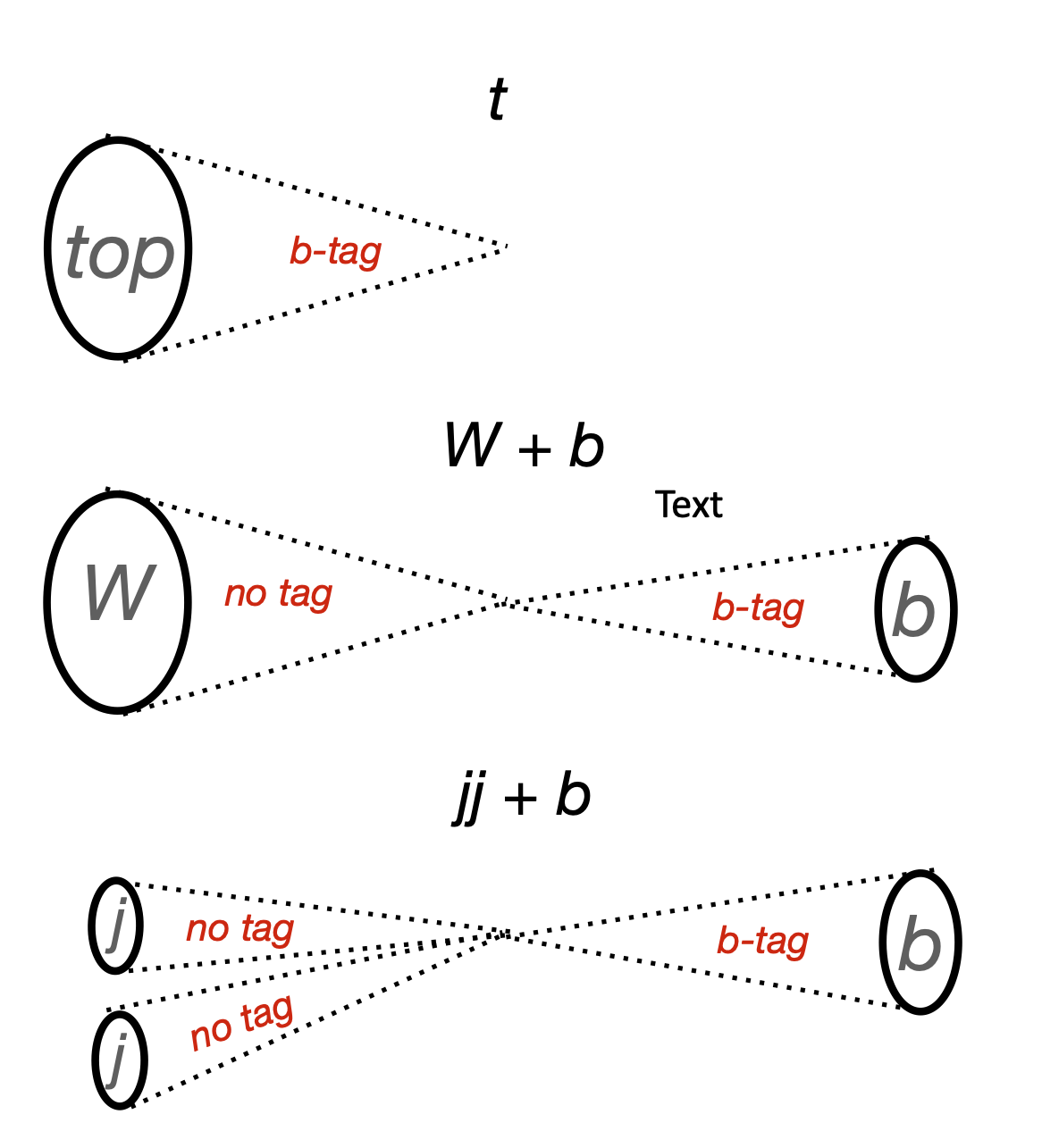
**Figure 7 |** Three possible top quark reconstruction strategies, using wide-cone and narrow-cone jets, which can be $b-$ tagged, $W$ -tagged or top-tagged. See text for details.

The three approaches are illustrated in Figure 7. If several reconstruction approaches are available for a single event, preference is given to t and then $W + b$ . If several jets are available within one approach, preference is given to the jets that minimize the difference between the reconstructed and known top-quark and $W-$ boson masses. Events with no T quark candidate with mass greater than 200 GeV are rejected. Distributions of reconstructed T quark candidate masses are shown in Figure 2 for two representative models.

Acknowledgment

DW was funded by the DOE Office of Science. The work of M.Fieg was supported by NSF Grant PHY2210283 and was also supported by NSF Graduate Research Fellowship Award No. DGE-1839285. The authors thank Tim Tait, Avik Roy, Jeong Han Kim and KC Kong for useful comments.

References

N. Arkani-Hamed, G. L. Kane, J. Thaler, and L.-T. Wang, JHEP 08, 070 (2006), hep-ph/0512190 [↩]
J. Alwall, P. Schuster, and N. Toro, Phys. Rev. D 79, 075020 (2009), 0810.3921 [↩]
G. Aad et al. (ATLAS), Phys. Lett. B 716, 1 (2012), 1207.7214 [↩]
S. Chatrchyan et al. (CMS), Phys. Lett. B 716, 30 (2012), 1207.7235 [↩]
G. Aad et al. (ATLAS), JHEP 07, 088 (2023), 2207.00348 [↩]
A. M. Sirunyan et al. (CMS), JHEP 07, 027 (2021), 2103.06956 [↩]
N. Craig, P. Draper, K. Kong, Y. Ng, and D. Whiteson, Acta Phys. Polon. B 50, 837 (2019), 1610.09392 [↩]
J. H. Kim, K. Kong, B. Nachman, and D. Whiteson, JHEP 04, 030 (2020), 1907.06659 [↩]
S. Tong, J. Corcoran, M. Fieg, M. Fenton, and D. Whiteson, JHEP 02, 057 (2024), 2311.00121 [↩]
J. H. Kim and I. M. Lewis, JHEP 05, 095 (2018), 1803.06351 [↩]
H. Alhazmi, J. H. Kim, K. Kong, and I. M. Lewis, JHEP 01, 139 (2019), 1808.03649 [↩] [↩] [↩]
M. Aaboud et al. (ATLAS), Phys. Rev. Lett. 121, 211801 (2018), 1808.02343 [↩]
M. Aaboud et al. (ATLAS), JHEP 10, 141 (2017), 1707.03347 [↩]
A. Tumasyan et al. (CMS), JHEP 09, 057 (2023), 2302.12802 [↩]
A. Tumasyan et al. (CMS), JHEP 05, 093 (2022), 2201.02227 [↩]
A. M. Sirunyan et al. (CMS), Phys. Rev. D 102, 112004 (2020), 2008.09835 [↩]
A. Roy, N. Nikiforou, N. Castro, and T. Andeen, Phys. Rev. D 101, 115027 (2020), 2003.00640 [↩]
G. Aad et al. (ATLAS), Phys. Rev. D 105, 092012 (2022), 2201.07045 [↩]
G. Aad et al. (ATLAS), JHEP 08, 153 (2023), 2305.03401 [↩]
G. Aad et al. (ATLAS), Eur. Phys. J. C 83, 719 (2023), 2212.05263 [↩]
G. Aad et al. (ATLAS), Phys. Rev. Lett. 131, 181901 (2023), 2302.01283 [↩]
J. a. M. Alves, G. C. Branco, A. L. Cherchiglia, C. C. Nishi, J. T. Penedo, P. M. F. Pereira, M. N. Rebelo, and J. I. Silva-Marcos (2023), 2304.10561 [↩]
J. A. Aguilar-Saavedra, R. Benbrik, S. Heinemeyer, and M. Pérez-Victoria, Phys. Rev. D 88 (2013), https://doi.org/10.1103/physrevd.88.094010 [↩]
B. A. Dobrescu and C. T. Hill, Phys. Rev. Lett. 81, 2634 (1998), hep-ph/9712319 [↩]
K. du Plessis, M. M. Flores, D. Kar, S. Sinha, and H. van der Schyf, SciPost Phys. 13, 018 (2022), 2112.08425 [↩]
M. Schmaltz and D. Tucker-Smith, Ann. Rev. Nucl. Part. Sci. 55, 229 (2005), hep-ph/0502182 [↩] [↩]
O. Witzel, PoS LATTICE2018, 006 (2019), 1901.08216 [↩]
B. Lillie, J. Shu, and T. M. P. Tait, JHEP 04, 087 (2008), 0712.3057 [↩] [↩]
A. Delgado and T. M. P. Tait, JHEP 07, 023 (2005), hep-ph/0504224 [↩]
K. Kumar, T. M. Tait, and R. Vega-Morales, JHEP 05, 022 (2009), 0901.3808 [↩]
A. Pomarol and J. Serra, Phys. Rev. D 78, 074026 (2008), 0806.3247 [↩]
A. Belyaev, R. S. Chivukula, B. Fuks, E. H. Simmons, and X. Wang, Phys. Rev. D 108, 035016 (2023), 2306.11097 [↩]
M. Aaboud et al. (ATLAS), Eur. Phys. J. C 78, 102 (2018), 1709.10440 [↩]
A. M. Sirunyan et al. (CMS), Phys. Lett. B 805, 135448 (2020), 1911.03761 [↩]
B. K. Sahoo, B. P. Das, and H. Spiesberger, Phys. Rev. D 103, L111303 (2021), 2101.10095 [↩]
J. Alwall, R. Frederix, S. Frixione, V. Hirschi, F. Maltoni, et al., JHEP 1407, 079 (2014), 1405.0301 [↩]
G. Cowan, K. Cranmer, E. Gross, and O. Vitells, Eur. Phys. J. C 71, 1554 (2011), Erratum: Eur.Phys.J.C 73, 2501 (2013), 1007.1727 [↩]
T. Junk, Nucl. Instrum. Meth. A 434, 435 (1999), hep-ex/9902006 [↩]
A. L. Read, J. Phys. G 28, 2693 (2002 [↩]
L. Heinrich, M. Feickert, and G. Stark, pyhf: v0.7.3, Zenodo (2020), https://doi.org/10.5281/zenodo.1169739 [↩]
L. Heinrich, M. Feickert, G. Stark, and K. Cranmer, Journal of Open Source Software 6, 2823 (2021), https://doi.org/10.21105/joss.02823 [↩]
C.-Y. Chen, S. Dawson, and I. Lewis, Phys. Rev. D 90 (2014), https://doi.org/10.1103/physrevd.90.035016 [↩]
C.-Y. Chen, S. Dawson, and E. Furlan, Phys. Rev. D 96 (2017), https://doi.org/10.1103/physrevd.96.015006 [↩]
S. Dawson and E. Furlan, Phys. Rev. D 86 (2012), https://doi.org/10.1103/physrevd.86.015021 [↩]
D. Choudhury, T. M. P. Tait, and C. E. M. Wagner, Phys. Rev. D 65, 053002 (2002), hep-ph/0109097 [↩]
K. Ishiwata, Z. Ligeti, and M. B. Wise, JHEP 2015, 027 (2015), https://doi.org/10.1007/jhep10(2015)027 [↩]
ATLAS Collaboration, Phys. Rev. D 98 (2018), https://doi.org/10.1103/physrevd.98.032002 [↩]
F. del Aguila and J. Cortés, Phys. Lett. B 156, 243 (1985), https://www.sciencedirect.com/science/article/pii/0370269385915175 [↩]
Z. Kang and Y. Shigekami, JHEP 2019, 049 (2019), https://doi.org/10.1007/jhep11(2019)049 [↩]
S. Balaji, JHEP 05, 015 (2022), 2110.05473 [↩]
Y. Okada and L. Panizzi, Adv. High Energy Phys. 2013, 364936 (2013), 1207.5607 [↩]
D. Gonçalves, K. Kong, and J. H. Kim, JHEP 06, 079 (2018), 1804.05874 [↩]
D. Gonçalves, J. H. Kim, K. Kong, and Y. Wu, JHEP 01, 158 (2022), 2108.01083 [↩]
A. Blondel et al. (2019), 1909.12245 [↩]
B. Norum and R. Rossmanith, Nucl. Phys. B Proc. Suppl. 51, 191 (1996), acc-phys/9604002 [↩]
J. Alwall, R. Frederix, S. Frixione, V. Hirschi, F. Maltoni, O. Mattelaer, H. S. Shao, T. Stelzer, P. Torrielli, and M. Zaro, JHEP 07, 079 (2014), 1405.0301 [↩]
R. D. Ball et al. (NNPDF), Eur. Phys. J. C 81, 958 (2021), 2109.02671 [↩]
T. Sjostrand, S. Mrenna, and P. Z. Skands, JHEP 0605, 026 (2006), hep-ph/0603175 [↩]
J. de Favereau et al. (DELPHES 3), JHEP 1402, 057 (2014), 1307.6346 [↩]
R. Brun and F. Rademakers, Nucl. Instrum. Meth. A 389, 81 (1997 [↩]
M. Cacciari, G. P. Salam, and G. Soyez, JHEP 04, 063 (2008), 0802.1189 [↩]
M. Cacciari, G. P. Salam, and G. Soyez, Eur. Phys. J. C 72, 1896 (2012), 1111.6097 [↩]
A. M. Sirunyan et al. (CMS), JHEP 04, 031 (2019), 1810.05905 [↩]
G. Aad et al. (ATLAS), JHEP 10, 061 (2020), 2005.05138 [↩]

Disentangling New Physics in Single Resonant Top Quarks

Abstract

Introduction