Creating Compositions in the Style of Henryk Wieniawski Using Generative AI

Abstract

Music is a fundamental part of various shared human experiences. In this paper, we aim to contribute to enhancing this experience by leveraging rapidly progressing AI technology to create music. Specifically, we recreate music in the style of Henryk Wieniawski using a custom-designed LSTM Sequential Generative AI Neural Network architecture. The AI generated music successfully mimicked Wieniawski’s style and created an arguably present impression. This work demonstrates how the influence of composers can persist beyond the grave, allowing their music to be enjoyed and intertwined with various modern styles and trends. It paves the steps for how AI generated and human made music can one day be indistinguishable.

Introduction

Throughout ages, music has been closely bonded with humans. It’s an intrinsic part of our shared human experience. In this new age of AI, this experience can be transferred to machines. This paper intends to explore that by looking at a prolific 19th century composer Henryk Wieniawski¹. This was as his music had been an integral part of the author’s journey of learning and playing music.

Since music composition is sequential in nature^{2,3,4,5,6,7,8}. and depends on continuing the pattern of coherence created by the previous notes, we decided that our architecture should follow this criterion. Hence we decided to use a generative sequence neural network.

Sequence models have made significant strides in the 2020s, with transformer models⁹ such as MuseNet taking the world by storm. However transformer models are complex to work with and expensive to train. Hence we use a simpler architecture:^10,11,12. LSTMs are a reasonably advanced and capable Recurrent Neural Network architecture that is capable of handling our sequential musical data: they can retain context over long durations and are capable of making predictions based on this past information. Thus LSTMs are suitable for our use case with handling sequential data and creating music in the style of Henryk Wieniawski.

Methods

For reasons of simplicity and practicality, we chose to implement our LSTM system using TensorFlow¹³. Particularly since much of the relevant Gen AI literature that we based our work on used TensorFlow

Discussion of the Dataset

Our input data was in the MIDI standard. The MIDI format is a convenient data for presenting music because of its small file size, ease of editing, and wide compatibility. MIDI files store instructions for music playback, including note pitches and timings. 

We used the broad Maestro dataset¹⁴, which consists of 200 hours of paired audio and MIDI recordings from ten years of International Piano-e-Competition., to pretrain the model in order to teach it basic musical theory, alongside a smaller dataset consisting of 8 handpicked compositions for violin by Henryk Wieniawski, which are used for the purpose of finetuning the model towards his style of composition. The Maestro dataset is ~201.2 hours of music long, while the Wieniawski one is ~1.1 hours. The pieces we used are shown in Table 1.

Wieniawski Violin Concerto Number 2

Wieniawski Violin Caprice no.18

Scherzo-Tarentelle Op.16

L’école moderne, Op.10

Wieniawski Op.15 Variations On An Original Theme

Wieniawski Etudes-Caprices 1-4 from Opus 18

Wieniawski Violin Concerto 1 Movement 1

The  input MIDI data was transformed into a set of values (duration, pitch, and step) using pretty_midi¹⁵, a Python library which provides an interface for dealing with the MIDI standard. This is a sensible embedding for both man and machine: it represents the contents of a musical sheet a human would be reading while learning how to play a piece, simultaneously capturing the core elements that a machine would require and need to understand as well. It might not necessarily be the optimal embedding possible, but it is a good starting point nevertheless. 

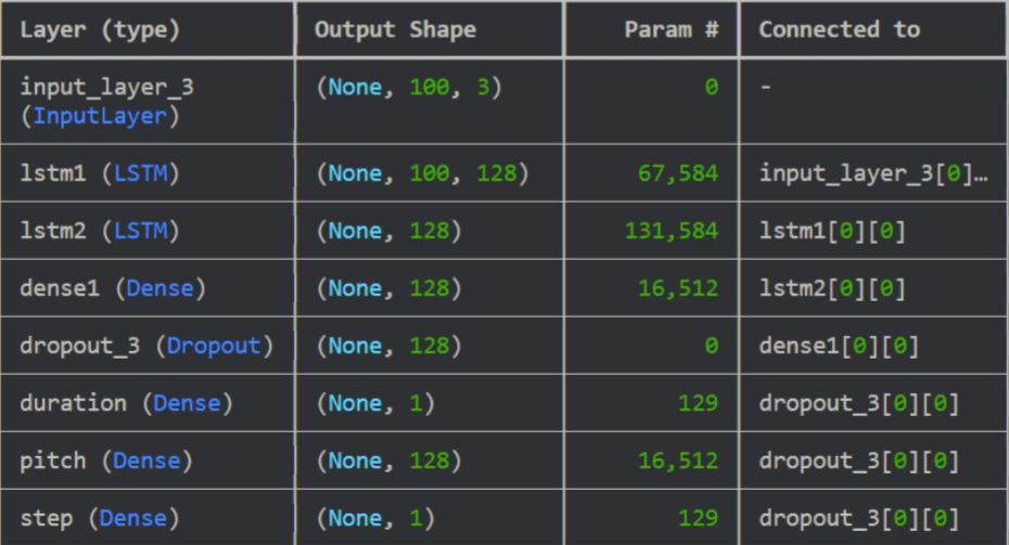
With regards to processing the data, our Neutral Network architecture consisted of 2 LSTM layers followed by a dense layer.  The purpose of the first layer is to capture the micro structure of the music i.e: short-range features and the logical flow of notes⁴.  

The second layer was  meant to be a layer that captured the overarching nature of the piece, such as the mood of the melody and compositional styles⁴. The final dense layer  takes the output of the 2nd layer and converts this into a musical output. 

To avoid overfitting of the model, dropout layers¹⁶ were incorporated, as shown in the visualisation of the entire model in Figure 1. Our loss function L was chosen such that the machine would focus on capturing the pitch, step and duration of the notes in a balanced way:

   

with L being the cross-entropy loss, being the mean squared error loss and a,b,c human-chosen weights. This architecture is capable of taking the embedded data and processing it in a systematic and sensible manner. 

We pretrained our model until L converged for the base Maestro dataset for different values of a, b and c hyperparameters. Each training run 24 epochs, at a batch-size of 45 minutes of music. Our evaluation of the model performance consisted of listening to the output manually instead of seeking to minimise the loss on some train/test data: this is because finding the absolute minimum of our (or, to our knowledge, any) quantitative loss function would not necessarily represent an ideal, objective human impression of the music. Quantifying how a human experiences music through a loss function is a highly challenging task indeed¹⁷ and well beyond the scope of this work. In the end, a favourite (a,b,c) combination was determined [see appendix] and fixed.
Following the creation of the pretrained NN, we incorporated Wieniawski’s musical style through transfer learning. This was done by allowing for select layers of the NN to be retrained on the 7 Wieniawski compositions. Three configurations were explored: only dense1 layer trainable, dense1 and lstm2 layers, and finally dense1, lstm2 and lstm1. Each retraining was done using 50 epochs, each time starting from the pretrained model.

Results / Discussion

The output of our generative NN were four musical MIDI files: the output of pretraining on Maestro, along with the results of the three transfer learning combinations. We first discuss the pretraining output, where all layers were trained on Maestro.The audio is characteristic of a piano due to the Maestro dataset being a collection of piano recordings (in contrast to the violin recordings of our Wieniawski). We regarded the audio to be mildly incoherent. In our opinion, it does not sound as pleasing as the other three outputs. Furthermore, we make the obvious observation that this audio displays no similarity to Wieniawski because it was trained on a dataset which included no pieces by the composer. Now we discuss the outputs from the transfer-learning on Wieniawski’s 7 compositions.

The output when only the dense1 layer was trainable suffers from a persistently low note, although the audio is coherent and structured. In other words, it is a sort of composition. However, the sections of the composition, i.e. the melodies, do not blend well with each other, making the overall piece sound subpar. This is reminiscent of the “stream of thought” issue that overly simple sequence models are known to suffer from, where parts of sentences or even whole sentences make sense, while the actual paragraph does not¹⁸. 

When the dense1 and lstm2 layers are trainable, the audio is still both slightly incoherent in some parts and suffers from a persistent low note, but to a lesser extent than when just the dense1 layer was trainable. There is variance in the tempo of the output but none in terms of dynamics. The sequences of notes follow each other logically in the short-term, but, again, not in the long-term.

Lastly, when enabling the training of the dense1, lstm2 and lstm1 layers, the output becomes generally coherent and the sequence of notes most logical. There are a few characteristic elements of Wieniawski such as string crossings and alternations between low and high pitched notes¹⁹. More musical elements such as variation in tempo are noticeable: suggesting that the lstm1 layer was a useful addition. Something resembling a motif can be observed: there are two melodies between which the output alternates. One issue with this output is that the ending is abrupt, unlike most classical music pieces which slow down – or become softer – towards the end. 

We found the final output to sound the best out of the four. We speculate this could be due to the neural network having a hot-start from the general Maestro datasets, and then properly fine-trained on 7 musical pieces that are consistent and much more correlated with each other than the disparate music in Maestro.

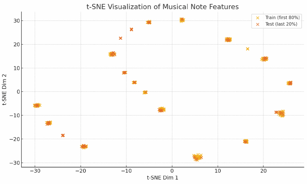
The t‑SNE plot shows clusters of notes with similar pitch (tone), duration (length), and step (time between notes), revealing structured musical patterns that the LSTM can learn and generalize from, with blue (train) and orange (test) dots occupying different regions, highlighting a shift in musical style.

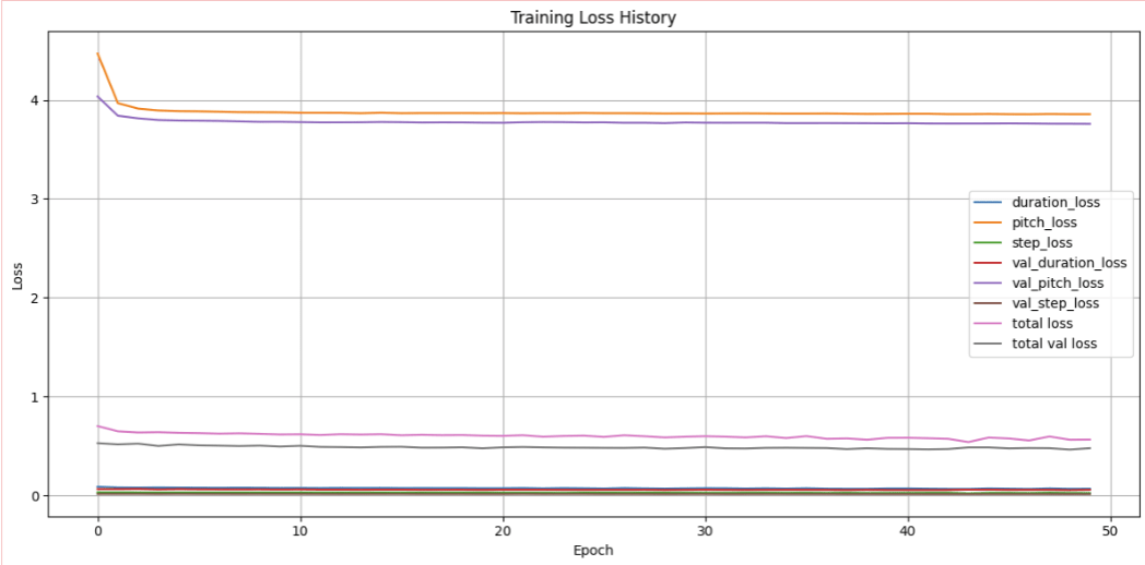
Figure 3 visualizes the model’s learning dynamics across 50 epochs. It shows the individual component losses (pitch_loss, step_loss, duration_loss) and their counterparts on the validation set (val_pitch_loss, etc.). The total loss (a weighted sum of the three outputs) is also shown for both training and validation, renamed here as “total loss” and “total val loss” for clarity. The losses generally exhibit convergence over time, with relatively small generalization gaps.

Conclusion

To summarise, we have here managed to create music, a deeply human pursuit, in the style of Wieniawski using AI. Such AIs can help a composer’s musical style continue to live on even after their death; in a sense, even resurrecting them in the form of an AI model. 

While our output was coherent, it lacked the true complexity and flair of Wieniawski. In the future, our model can be iterated on by using transformer layers instead of LSTMs, adjusting the loss function,improving data quality and size, and formulating an automated cross-validation scheme to minimise human involvement in evaluating our model performance. In the future, we envision further advances in generative AI for music generation²⁰, allowing great renditions of the historical composers and their works²¹, and even novel compositions that will strike at the heart of humans²².

Appendix: Source Code

!pip install pretty_midi


# Library Installations
import os.path
import tensorflow as tf
from tensorflow.keras.layers import Input, LSTM, Dense, Dropout
from tensorflow.keras.models import Model
from tensorflow.keras.losses import SparseCategoricalCrossentropy
from tensorflow.keras.optimizers.schedules import PiecewiseConstantDecay
from tensorflow.keras.optimizers import Adam


from typing import Dict, List, Optional, Sequence, Tuple
import collections
import datetime
import glob
import numpy as np
import pathlib
import pandas as pd
import pretty_midi
from matplotlib import pyplot as plt






# Hyperparameters
seq_length = 100
vocab_size = 500
batch_size = 256
epochs = 1
temperature = 2.0
num_predictions = 400
# Pre-train vs fine-tune flag
PRETRAIN = False
learning_rate = 0.003 if PRETRAIN else 0.001
# Dataset Prep
seed = 42
tf.random.set_seed(seed)
np.random.seed(seed)


# Setting the path and loading the data


if PRETRAIN:
    data_dir = pathlib.Path('maestro-v2.0.0-midi/maestro-v2.0.0')
    filenames = glob.glob(str(data_dir/'**/*.mid*'))
else:
    data_dir = pathlib.Path('finetrained')
    filenames = glob.glob(str(data_dir/'*.mid*'))
print('Number of files:', len(filenames))


# analyzing and working with a sample file
try:
    sample_file = filenames[1]
except:
    sample_file = filenames[0]
pm = pretty_midi.PrettyMIDI(sample_file)
instrument = pm.instruments[0]
instrument_name = pretty_midi.program_to_instrument_name(instrument.program)




# Extracting the notes
for i, note in enumerate(instrument.notes[:10]):
    note_name = pretty_midi.note_number_to_name(note.pitch)
    duration = note.end - note.start




# Extracting the notes from the sample MIDI file


def midi_to_notes(midi_file: str) -> pd.DataFrame:
    pm = pretty_midi.PrettyMIDI(midi_file)
    instrument = pm.instruments[0]
    notes = collections.defaultdict(list)


    # Sort the notes by start time
    sorted_notes = sorted(instrument.notes, key=lambda note: note.start)
    prev_start = sorted_notes[0].start


    for note in sorted_notes:
        start = note.start
        end = note.end
        notes['pitch'].append(note.pitch)
        notes['start'].append(start)
        notes['end'].append(end)
        notes['step'].append(start - prev_start)
        notes['duration'].append(end - start)
        prev_start = start


    return pd.DataFrame({name: np.array(value) for name, value in notes.items()})


raw_notes = midi_to_notes(sample_file)
raw_notes.head()


# Converting to note names by considering the respective pitch values


get_note_names = np.vectorize(pretty_midi.note_number_to_name)
sample_note_names = get_note_names(raw_notes['pitch'])




# Visualizing the paramaters of the muscial notes of the piano
def plot_piano_roll(notes: pd.DataFrame, count: Optional[int] = None):
    if count:
        title = f'First {count} notes'
    else:
        title = f'Whole track'
        count = len(notes['pitch'])


        plt.figure(figsize=(20, 4))
        plot_pitch = np.stack([notes['pitch'], notes['pitch']], axis=0)
        plot_start_stop = np.stack([notes['start'], notes['end']], axis=0)


        plt.plot(plot_start_stop[:, :count], plot_pitch[:, :count], color="b", marker=".")
        plt.xlabel('Time [s]')
        plt.ylabel('Pitch')
        _ = plt.title(title)




# Training Data Creation
def notes_to_midi(notes: pd.DataFrame, out_file: str, instrument_name: str,
                  velocity: int = 100) -> pretty_midi.PrettyMIDI:


    pm = pretty_midi.PrettyMIDI()
    instrument = pretty_midi.Instrument(
      program=pretty_midi.instrument_name_to_program(
          instrument_name))


    prev_start = 0
    for i, note in notes.iterrows():
        start = float(prev_start + note['step'])
        end = float(start + note['duration'])


        note = pretty_midi.Note(velocity=velocity, pitch=int(note['pitch']),
                                start=start, end=end)
        instrument.notes.append(note)
        prev_start = start


    pm.instruments.append(instrument)
    pm.write(out_file)
    return pm


example_file = 'example.midi'
example_pm = notes_to_midi(
    raw_notes, out_file=example_file, instrument_name=instrument_name)


num_files = 5
all_notes = []
for f in filenames[:num_files]:
    notes = midi_to_notes(f)
    all_notes.append(notes)


all_notes = pd.concat(all_notes)


n_notes = len(all_notes)


key_order = ['pitch', 'step', 'duration']
train_notes = np.stack([all_notes[key] for key in key_order], axis=1)


notes_ds = tf.data.Dataset.from_tensor_slices(train_notes)
notes_ds.element_spec


def create_sequences(dataset: tf.data.Dataset, seq_length: int,
                     vocab_size = 128) -> tf.data.Dataset:
    """Returns TF Dataset of sequence and label examples."""
    seq_length = seq_length+1


    # Take 1 extra for the labels
    windows = dataset.window(seq_length, shift=1, stride=1,
                              drop_remainder=True)


    # `flat_map` flattens the" dataset of datasets" into a dataset of tensors
    flatten = lambda x: x.batch(seq_length, drop_remainder=True)
    sequences = windows.flat_map(flatten)


    # Normalize note pitch
    def scale_pitch(x):
        x = x/[vocab_size,1.0,1.0]
        return x


    # Split the labels
    def split_labels(sequences):
        inputs = sequences[:-1]
        labels_dense = sequences[-1]
        labels = {key:labels_dense[i] for i,key in enumerate(key_order)}


        return scale_pitch(inputs), labels


    return sequences.map(split_labels, num_parallel_calls=tf.data.AUTOTUNE)


seq_ds = create_sequences(notes_ds, seq_length, vocab_size)






buffer_size = n_notes - seq_length  # the number of items in the dataset
train_ds = (seq_ds
            .shuffle(buffer_size)
            .batch(batch_size, drop_remainder=True)
            .cache()
            .prefetch(tf.data.experimental.AUTOTUNE))


# Making the model
def mse_with_positive_pressure(y_true: tf.Tensor, y_pred: tf.Tensor):
    mse = (y_true - y_pred) ** 2
    positive_pressure = 10 * tf.maximum(-y_pred, 0.0)
    return tf.reduce_mean(mse + positive_pressure)


# Developing the model


input_shape = (seq_length, 3)


inputs = Input(input_shape)
# x = LSTM(128,
#          return_sequences=False,
#          dropout=0.2,            # Dropout for inputs
#          recurrent_dropout=0.2   # Dropout for recurrent state
#          )(inputs)






x = LSTM(128, return_sequences=True, name='lstm1',
         dropout=0.2, recurrent_dropout=0.2)(inputs)
# Second LSTM layer (to be trained)
x = LSTM(128, name='lstm2',
         dropout=0.2, recurrent_dropout=0.2)(x)
x = Dense(128,name='dense1', activation = 'relu')(x)
x = Dropout(0.2)(x)
outputs = {'pitch': Dense(128, name='pitch')(x),
          'step': Dense(1, name='step')(x),
          'duration': Dense(1, name='duration')(x),
          }






model = Model(inputs, outputs)


if PRETRAIN:
    if os.path.isfile("pretrained_musical_lstm.weights.h5"):
        model.load_weights("pretrained_musical_lstm.weights.h5")
else:
    if os.path.isfile("finetrained_musical_lstm.weights.h5"):
        model.load_weights("finetrained_musical_lstm.weights.h5")
    else:
        model.load_weights("pretrained_musical_lstm.weights.h5")
loss = {'pitch': SparseCategoricalCrossentropy(from_logits=True),
        'step': mse_with_positive_pressure,
        'duration': mse_with_positive_pressure,
      }


optimizer = Adam(learning_rate=learning_rate)
model.compile(loss=loss, optimizer=optimizer)
model.summary()


# Compiling and fitting the model
model.compile(loss = loss,
              loss_weights = {'pitch': 0.05, 'step': 4.0, 'duration':4.0,},
              optimizer = optimizer)


history = model.fit(train_ds, epochs=epochs)


if PRETRAIN: model.save_weights("pretrained_musical_lstm.weights.h5")
else: model.save_weights("finetrained_musical_lstm.weights.h5")




# Freezing the first two LSTM layers in case of PRETRAIN being false
if not PRETRAIN:
    model.get_layer('lstm1').trainable = False
    model.get_layer('lstm2').trainable = True
    # after 100 epoch, save then finetuned file as "finetuned both layers untrainable"
    # then set lstm2 trainable to true and train for 100 more and then see how it differs. save that as finetuned last layer trainable




if PRETRAIN: model.load_weights("pretrained_musical_lstm.weights.h5")
else: model.load_weights("finetrained_musical_lstm.weights.h5")
# Generating the notes
def predict_next_note(notes: np.ndarray, keras_model: tf.keras.Model,
                      temperature: float = 1.0) -> int:
    """Generates a note IDs using a trained sequence model."""


    assert temperature > 0


    # Add batch dimension
    inputs = tf.expand_dims(notes, 0)


    predictions = model.predict(inputs)
    pitch_logits = predictions['pitch']
    step = predictions['step']
    duration = predictions['duration']


    pitch_logits /= temperature
    pitch = tf.random.categorical(pitch_logits, num_samples=1)
    pitch = tf.squeeze(pitch, axis=-1)
    duration = tf.squeeze(duration, axis=-1)
    step = tf.squeeze(step, axis=-1)


    # `step` and `duration` values should be non-negative
    step = tf.maximum(0, step)
    duration = tf.maximum(0, duration)


    return int(pitch), float(step), float(duration)


sample_notes = np.stack([raw_notes[key] for key in key_order], axis=1)


# The initial sequence of notes while the pitch is normalized similar to training sequences
input_notes = (
    sample_notes[:seq_length] / np.array([vocab_size, 1, 1]))


generated_notes = []
prev_start = 0


for _ in range(num_predictions):
    pitch, step, duration = predict_next_note(input_notes, model, temperature)
    start = prev_start + step
    end = start + duration
    input_note = (pitch, step, duration)
    generated_notes.append((*input_note, start, end))
    input_notes = np.delete(input_notes, 0, axis=0)
    input_notes = np.append(input_notes, np.expand_dims(input_note, 0), axis=0)
    prev_start = start


generated_notes = pd.DataFrame(
    generated_notes, columns=(*key_order, 'start', 'end'))


generated_notes.head(10)


out_file = 'output.midi'
out_pm = notes_to_midi(
    generated_notes, out_file=out_file, instrument_name=instrument_name)

References

1. The Editors of Encyclopedia Britannica. (2025). Henryk Wieniawski. In Encyclopædia Britannica [↩]
2. Huang, C.-Z. A., Vaswani, A., Uszkoreit, J., Shazeer, N., Simon, I., Hawthorne, C., Dai, A. M., Hoffman, M. D., Dinculescu, M., & Eck, D. (2019). Music Transformer: Generating Music with Long-Term Structure. In Proceedings of the 7th International Conference on Learning Representations (ICLR 2019). [↩]
3. van den Oord, A., Dieleman, S., Zen, H., Simonyan, K., Vinyals, O., Graves, A., Kalchbrenner, N., Senior, A., Kavukcuoglu, K., & van den Oord, A. (2016). WaveNet: A Generative Model for Raw Audio. DeepMind Technical Report (arXiv:1609.03499), 2016. [↩]
4. Dong, H.-W., Hsiao, W.-Y., Yang, L.-C., & Yang, Y.-H. (2018). MuseGAN: Multi-track Sequential Generative Adversarial Networks for Symbolic Music Generation and Accompaniment. In Proceedings of the Thirty-Second AAAI Conference on Artificial Intelligence (AAAI 2018) (pp. 34–41). [↩] [↩] [↩]
5. Dhariwal, P., Jun, H., Payne, C., Kim, J. W., Radford, A., & Sutskever, I. (2020). Jukebox: A Generative Model for Music. In Proceedings of the 37th International Conference on Machine Learning (ICML 2020) (Vol. 119, pp. 2701–2710). [↩]
6. Cope, D. (1991). Experiments in Musical Intelligence. A-R Editions [↩]
7. Briot, J.-P., Hadjeres, G., & Pachet, F.-D. (2019). Deep Learning Techniques for Music Generation: A Survey. IEEE Computational Intelligence Magazine, 13(3), 14–24. (Original arXiv preprint arXiv:1709.01620v4). [↩]
8. Cuthbert, M. S., & Ariza, C. (2010). music21: A Toolkit for Computer-Aided Musicology and Symbolic Music Data. In Proceedings of the 11th International Society for Music Information Retrieval Conference (ISMIR 2010) (pp. 637–642). [↩]
9. Vaswani, A., Shazeer, N., Parmar, N., Uszkoreit, J., Jones, L., Gomez, A. N., Kaiser, Ł., & Polosukhin, I. (2017). Attention Is All You Need. In Advances in Neural Information Processing Systems 30 (NIPS 2017) pp. 5998–6008 [↩]
10. Long Short Term Memory (LSTMs) Hochreiter, S., & Schmidhuber, J. (1997). Long Short-Term Memory. Neural Computation, 9(8), 1735–1780 [↩]
11. Eck, D., & Schmidhuber, J. (2002). Finding Temporal Structure in Music: Blues Improvisation with LSTM Recurrent Neural Networks. In Proceedings of the IEEE Workshop on Neural Networks for Signal Processing (NNSP 2002) (pp. 747–752). [↩]
12. Sutskever, I., Vinyals, O., & Le, Q. V. (2014). Sequence to Sequence Learning with Neural Networks. In Advances in Neural Information Processing Systems 27 (NIPS 2014) (pp. 3104–3112). [↩]
13. Abadi, et al (2016). TensorFlow: A System for Large-Scale Machine Learning. In Proceedings of the 12th USENIX Symposium on Operating Systems Design and Implementation (OSDI 2016) pp. 265–283 [↩]
14. Hawthorne, C., Stasyuk, A., Roberts, A., Simon, I., Huang, C.-Z. A., Dieleman, S., Elsen, E., Engel, J., & Eck, D. (2018). Enabling Factorized Piano Music Modeling and Generation with the MAESTRO Dataset. In Proceedings of the 35th International Conference on Machine Learning (ICML 2018) Vol. 80, pp. 710–719 [↩]
15. Raffel, C., & Ellis, D. P. W. (2014). Intuitive Analysis, Creation and Manipulation of MIDI Data with pretty_midi. In Proceedings of the 15th International Society for Music Information Retrieval Conference, Late-Breaking and Demo Papers, ISMIR 2014 [↩]
16. Srivastava, N., Hinton, G., Krizhevsky, A., Sutskever, I., & Salakhutdinov, R. (2014). Dropout: A simple way to prevent neural networks from overfitting. Journal of Machine Learning Research, 15(1), 1929–1958 [↩]
17. Zhang, H., Liang, J., Phan, H., Wang, W., & Benetos, E. (2025). From aesthetics to human preferences: Comparative perspectives of evaluating text-to-music systems. arXiv [↩]
18. Guan, J., Mao, X., Fan, C., Liu, Z., Ding, W., & Huang, M. (2021). Long text generation by modeling sentence-level and discourse-level coherence. In Proceedings of the 59th Annual Meeting of the Association for Computational Linguistics and the 11th International Joint Conference on Natural Language Processing (Volume 1: Long Papers) (pp. 6379–6393). Association for Computational Linguistics [↩]
19. Kozak, P. (2011). Pedagogical examination of Henryk Wieniawski’s L’école moderne Opus 10 (Doctoral dissertation). University of Georgia [↩]
20. Zhang, Y., Li, X., Wang, Z., & Chen, Y. (2024). Applications and Advances of Artificial Intelligence in Music Generation: A Systematic Review. arXiv preprint arXiv:2409.03715 [↩]
21. Kong, M., & Huang, L. (2021). Bach Style Music Authoring System based on Deep Learning. arXiv preprint arXiv:2110.02640 [↩]
22. Agres, K. R., Dash, A., & Chua, P. (2023). AffectMachine-Classical: A novel system for generating affective classical music. arXiv preprint arXiv:2304.04915 [↩]