Comparative Analysis of Machine Learning Models for Air Quality Index Prediction

July 19, 2025

954

Abstract

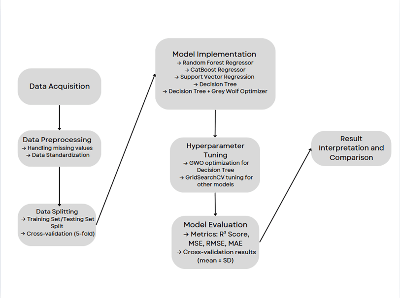
This research evaluates the performance of machine learning models in forecasting the Air Quality Index (AQI) using data from Amravati, Maharashtra, India. With air pollution contributing to millions of deaths annually, accurate AQI prediction is vital for timely interventions and public health protection. Existing models—ranging from traditional statistical approaches to standard machine learning algorithms—often struggle to capture the complex, non-linear relationships between pollutants, especially in data-constrained environments. To address these limitations, this study assesses five regression models: Random Forest Regressor, CatBoost Regressor, Support Vector Regression (SVR), Decision Tree Regressor, and a Decision Tree Regressor optimized using the Grey Wolf Optimization (GWO) algorithm. Models, except the GWO-optimized version, were fine-tuned using GridSearchCV and validated with 5-fold cross-validation. Performance was measured using standard metrics: coefficient of determination (R²), Mean Squared Error (MSE), Mean Absolute Error (MAE), and Root Mean Squared Error (RMSE).

Among the models, the GWO-optimized Decision Tree achieved the highest performance, with an R² of 0.9896, RMSE of 5.9063, MSE of 34.8846, and MAE of 2.3480. In contrast, SVR recorded the weakest results. The findings demonstrate the potential of metaheuristic optimization in boosting model accuracy and emphasize the importance of interpretable, data-efficient solutions for AQI forecasting in resource-limited areas.

Introduction

Air pollution remains one of the most pressing global challenges today, responsible for over 8.1 million deaths in 2021 and ranking as the second leading risk factor for mortality, including among vulnerable groups such as children under five years old¹^,². By anticipating air pollution spikes through predictive modeling, health agencies can warn populations, distribute protective resources, and also intervene in the short-term, closing schools or advising work-from-home, to reduce population exposure. Studies have shown that such actions can lower the number of emergency hospital visits³^,⁴^,⁵. They also improve respiratory health outcomes, especially within high-risk pollution events.

With advances in Artificial Intelligence (AI) and Machine Learning (ML), predicting air quality has become more efficient, offering data-driven insights for pollution control⁶. Despite their promise, current AQI forecasting methods face notable limitations. Traditional statistical models like linear regression and ARIMA often fail to capture the complex, non-linear interactions among pollutants⁷. While machine learning models like Random Forest and SVR perform better, they are highly sensitive to hyperparameter tuning, and are prone to overfitting or underfitting⁸. Many high-performing models such as deep neural networks lack interpretability and require substantial computational resources⁹, which limits their practical deployment—especially in smaller cities with limited infrastructure and datasets. These challenges highlight the need for interpretable, data-efficient models that are optimized using adaptive strategies to improve both accuracy and generalizability¹⁰.

Various machine learning models can be applied for predicting air pollution, each with its own set of advantages and disadvantages. The best model for a particular application depends on several factors: the quality and size of the dataset, the specific pollutants being measured, additional environmental data like meteorological conditions and the relationship between different pollutants. This study investigates the effectiveness of various ML models in predicting the Air Quality Index (AQI) using pollutant concentration data. Traditional machine learning models such as Random Forest (RF), CatBoost (CB), and Support Vector Regression (SVR) were optimized to ensure robust hyperparameter tuning using GridSearch with cross-validation. A novel approach involving Grey Wolf Optimization (GWO) was applied to optimize the parameters of a Decision Tree Regressor (DT). All models were evaluated using both test-set performance and 5-fold cross-validation, allowing for a comprehensive and reliable comparison of predictive accuracy. By identifying the most accurate model, this study contributes to improved air pollution forecasting, enabling more informed decision-making for public health and environmental policies.

Literature Summary

A variety of machine learning and deep learning approaches for forecasting AQI and specific pollutants have been studied. Garbagna et al.¹¹ conducted a comprehensive review of AI-driven approaches for air pollution modeling, highlighting the comparative strengths of Random Forest, SVR, and boosting techniques like XGBoost and CatBoost in temporal and spatiotemporal prediction tasks. The study’s findings emphasize the role of external features such as meteorological and traffic data in improving model performance, and the limitations of models in handling data imbalance and real-world variability. A study by Alsayadi et al.¹² conducted a comparative evaluation of regression models for forecasting AQI.

Metaheuristic hyperparameter optimization uses nature-inspired algorithms—such as Genetic Algorithms (GA), Particle Swarm Optimization (PSO), and Grey Wolf Optimization (GWO)—to effectively explore the hyperparameter space of machine learning models. These algorithms are designed to balance exploration and exploitation to find optimal or near-optimal parameter configurations¹³. Unlike traditional methods such as grid or random search, metaheuristics are more adaptable to complex, non-convex search spaces. Recent research has applied these techniques to address issues like overfitting and ineffective parameter tuning. Murillo-Escobar et al.¹⁴ demonstrated that a PSO-optimized SVR model could effectively forecast concentrations of multiple pollutants, showing strong year-round performance even under varying weather conditions with relatively low computational demands. Hilal et al.¹⁵ implemented a hybrid algorithm combining Decision Tree J48 and Grey Wolf Optimization for environmental pollution control. The DT-GWO model achieved a prediction accuracy of 99.78%, outperforming the standalone Decision Tree J48 (93.72%) and GWO (96.83%) models.

Methods

Overview of AQI Calculation

Interpreting air pollution data remains a challenge for the general public. To remedy this, Air Quality Index (AQI) is a tool for the simplification and effective communication of air quality status to people. It transforms complex air quality data of various pollutants into a single easy-to-understand number. The pollutants taken into consideration for AQI calculation are PM_2.5, PM₁₀, NO₂, NH₃, SO₂, CO, and Ozone. Each pollutant has a defined sub-index with its breakpoints defined. A sub-index value is calculated for each individual pollutant based on the breakpoint values using the following formula:

(1) $\begin{equation*}I = \left( \frac{I_{\text{high}} - I_{\text{low}}}{C_{\text{high}} - C_{\text{low}}} \right) (C - C_{\text{low}}) + I_{\text{low}}\end{equation*}$

Where; I = Sub-index value, C = Concentration of the pollutant, Clow= Lower concentration bound of the pollutant’s range, Chigh= Upper concentration bound of the pollutant’s range, $I_{low}$ = Lower sub-index breakpoint, Ihigh= Upper sub-index breakpoint¹⁶.

By Indian Central Pollution Control Board standards, the worst-case sub-index is considered as the final AQI¹⁶.

Tools

This research used the Jupyter Notebook editor for Python programming. To collect the data used for this research, air quality data for Amravati, Maharashtra, India, was sourced from the Central Pollution Control Board’s official database, covering the period from May 31, 2023, to February 15, 2025. The dataset includes key pollutants such as PM_2.5, PM₁₀, NO₂, NH₃, SO₂, CO, and Ozone. The following libraries were used for data manipulation, model implementation, evaluation, and visualization: Pandas, NumPy, Matplotlib, Seaborn, Scikit-learn components and CatBoost. The code used for data processing and analysis is available in a public GitHub repository (https://github.com/SaraiDeshmukh/AQI_Prediction_Code).

Data Preprocessing

To ensure data consistency, a thorough preprocessing was conducted. This included cleaning the dataset by removing duplicate records. Such preprocessing steps are necessary to maintain the accuracy and reliability of the data. The ‘From Date’ and ‘To Date’ columns, which initially presented redundant information, were converted into a single ‘Date’ column. This column was then formatted uniformly in the DD-MM-YYYY format for consistency across the entire dataset, facilitating easier analysis. To enhance the analysis further, the AQI (see Equation 1) was computed using a Python script, based on the pollutant concentrations for each date in the dataset. The calculated AQI values were subsequently added as an additional column to the dataset.

Model Training and Evaluation

An 80:20 split was used to separate the dataset into training and testing sets in order to assess the prediction power of several machine learning models. This ratio ensures that the model is trained on sufficiently large data, while also being tested on a separate, unseen portion to gauge its ability¹⁷. Recent research works on air quality prediction were considered for literature analysis.The methods used in each research work were studied and compared to find the best model for AQI prediction¹⁸^,¹⁹^,²⁰^,²¹.

While ensemble and hybrid models are known for their predictive strength¹⁵^,²², this study deliberately focuses on individual machine learning models to preserve interpretability, reduce computational complexity, and ensure ease of deployment in practical settings¹⁰. The selected models—RF, SVR, DT, CB—were chosen based on their proven track record in AQI prediction tasks¹⁹ as well as their balance between accuracy and transparency²³.

For the DT, two versions were considered:

1. An unoptimized baseline, trained with default parameters.

2. An optimized variant using Grey Wolf Optimization (DT+GWO), a metaheuristic algorithm. The GWO algorithm was integrated with 5-fold cross-validation during its objective evaluation, enabling it to search for the best values of hyperparameters for DT in a performance-guided manner .

To ensure robust performance and fair comparison; for RF, CB, and SVR, GridSearch with 5-fold Cross-Validation (GridSearchCV) was employed to systematically explore a predefined set of hyperparameters. This allowed each model to identify optimal parameter combinations and avoid overfitting²⁴. Importantly, 5-fold cross-validation was applied not only during the hyperparameter tuning process but also post-training, to compare models in terms of stability and average performance across multiple folds.

Model	Train/Test Split	Hyperparameters	Optimization Method
Random Forest (RF)	80% / 20%	n_estimators=100, max_depth=30, min_samples_split=2, min_samples_leaf=1, random_state=42	Grid Search CV (5-fold)
CatBoost (CB)	80% / 20%	iterations=100, depth=6, learning_rate=0.1, loss_function=’RMSE’	Grid Search CV (5-fold)
Support Vector Regression (SVR)	80% / 20%	kernel=’rbf’, C=1000, epsilon=0.1	Grid Search CV (5-fold)
Decision Tree (Optimized with GWO)	80% / 20%	max_depth=13, min_samples_split=3	Grey Wolf Optimizer
Decision Tree (Unoptimized)	80% / 20%	Default (max_depth=None, min_samples_split=2, etc.)	Not optimized

Table 1. Hyperparameter Settings and Optimization Methods for Evaluated Machine Learning Models

Each model was trained using the training dataset. The models were subsequently tested on the unseen dataset, and their predictive accuracy was evaluated using the coefficient of determination (R²), Mean Squared Error (MSE), Mean Absolute Error (MAE), and Root Mean Squared Error (RMSE).

Metrics used

⦁ R² (R-Squared)

R² explains the proportion of variance in the dependent variable that is predictable from the independent variables.

(2) $\begin{equation*}R^2 = 1 - \frac{\sum_{i=1}^{N} (y_i - \hat{y}<em>i)^2}{\sum</em>{i=1}^{N} (y_i - \bar{y})^2}\end{equation*}$

Where; N is the number of samples, $y_{i}$ are the actual observed values, $\hat{y}_{i}$ are the predicted values from the model, $\hat{y}$ is the mean of the actual observed values.

A value of $R^{2}$ close to 1 means that most of the variability in the response variable is explained by the model. $R^{2}$ alone can sometimes be misleading, especially in the presence of overfitting²⁵.

⦁ RMSE (Root Mean Squared Error)

RMSE measures the average magnitude of the errors between the actual and predicted values.

(3) $\begin{equation*}\text{RMSE} = \sqrt{ \frac{1}{N} \sum_{i=1}^{N} (y_i - \hat{y}_i)^2 }\end{equation*}$

Where; N is the number of samples, $y_{i}$ are the actual values, $\hat{y}_{i}$ are the predicted values.

It penalizes large errors more than smaller ones due to the squaring term. It is in the same units as the target variable.

⦁ MSE (Mean Squared Error)

MSE measures the average squared difference between the actual and predicted values.

(4) $\begin{equation*}\text{MSE} = \frac{1}{N} \sum_{i=1}^{N} (y_i - \hat{y}_i)^2\end{equation*}$

Where; N is the number of samples, $y_{i}$ are the actual values, $\hat{y}_{i}$ are the predicted values.

MSE gives a sense of how much the predicted values deviate from the true values, in the squared units of the target variable.

⦁ MAE (Mean Absolute Error)

MAE measures the average magnitude of the errors in a set of predictions, without considering their direction.

(5) $\begin{equation*}\text{MAE} = \frac{1}{N} \sum_{i=1}^{N} \left| y_i - \hat{y}_i \right|\end{equation*}$

Where; N is the number of samples, $y_{i}$ are the actual values, $\hat{y}_{i}$ are the predicted values.

MAE is the average of the absolute differences between predicted and actual values. Unlike MSE and RMSE, it does not penalize large errors more than smaller ones and is in the same units as the target variable.

Results

The research considered data from Amravati, Maharashtra, consisting of key pollutants, namely PM_2.5, PM₁₀, NO₂, NH₃, SO₂, CO, and Ozone spanning from May 31, 2023, to February 15, 2025.
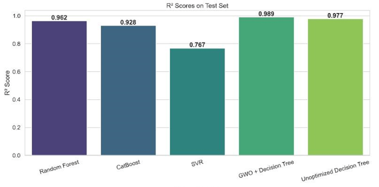
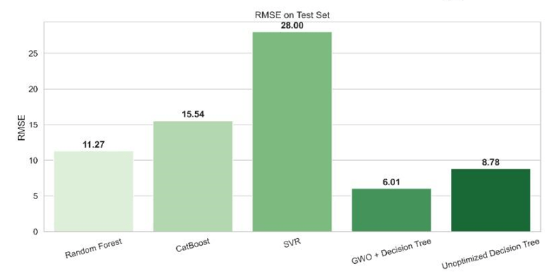
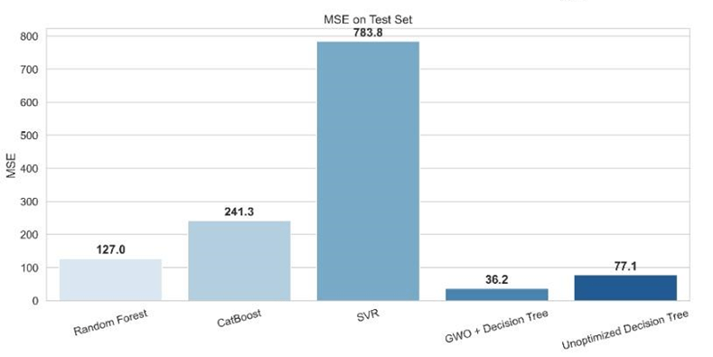
This dataset was used to train and evaluate the models. Among the five evaluated models, the DT+GWO demonstrated the best performance, showing the highest R² value (see Equation 2) and the lowest MSE (see Equation 4) and RMSE (see Equation 3) scores. It has a relatively high MAE (see Equation 5). RF and CB exhibited moderate predictive accuracy, whereas SVR performed the worst with relatively higher error metrics (MSE and RMSE) and R² value farthest away from 1. The unoptimized DT performed competitively with a high R², closely trailing the optimized DT+GWO model and outperforming SVR, CB and RF.

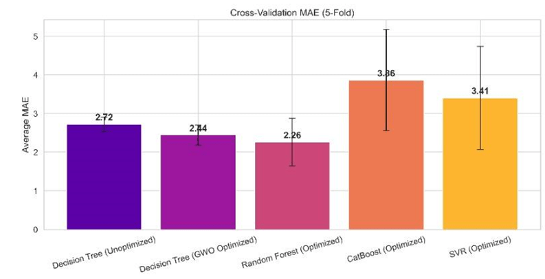
A 5-fold cross-validation was performed on all models. The results highlight consistent performance across folds, particularly for the RF and DT+GWO, both of which maintained high mean R² scores and relatively low variance. The unoptimized DT also performed well, showing minimal performance drop without optimization. CB achieved reasonable accuracy but exhibited higher variance. SVR showed competitive performance but with noticeable variability across folds.

Model	R² Score	MSE	RMSE	MAE
Decision Tree (GWO Optimized)	0.9896	34.88	5.91	2.35
Random Forest (Optimized)	0.9622	127.01	11.27	3.55
CatBoost (Optimized)	0.9283	241.34	15.54	6.16
Decision Tree (Unoptimized)	0.9775	75.83	8.71	2.92
Support Vector Regression (SVR)	0.7670	783.82	27.99	8.08

Table 2. Performance Metrics of Machine Learning Models for AQI Prediction

Model	Mean R²	R² Std. Dev.	Mean MAE	MAE Std. Dev.
Decision Tree (GWO Optimized)	0.9824	±0.0061	2.6904	±0.3093
Random Forest (Optimized)	0.9858	±0.0105	2.2612	±0.6116
CatBoost (Optimized)	0.9727	±0.0263	3.8627	±1.3087
Decision Tree (Unoptimized)	0.9812	±0.0046	2.5988	±0.3426
Support Vector Regression (SVR)	0.9656	±0.0321	3.4050	±1.3363

Table 3. Cross-Validation Performance Metrics (5-Fold) of Machine Learning Models for AQI Prediction

Figure 2. Coefficient of Determination (R²) on Test Dataset Across Models

Figure 3. Mean Absolute Error (MAE) on Test Dataset Across Models

Figure 4. Root Mean Squared Error (RMSE) on Test Dataset Across Models

Figure 5. Mean Squared Error (MSE) on Test Dataset Across Models

Figure 6. Average Cross-Validated R² Scores (5-Fold CV) with Error Margins

Figure 7. Average Cross-Validated MAE Scores (5-Fold CV) with Error Margins

Discussion

The results of the metrics demonstrated the DT+GWO to be the most accurate. CB and RF did not perform well, likely due to the fact that the relationship between different pollutants and the AQI is non-linear and complex. While both CB and RF are powerful models capable of capturing non-linearities, the specific way in which pollutants interact with AQI may still pose a challenge. For instance, a small increase in one pollutant might have a disproportionate impact on AQI, while a larger increase in another pollutant might not result in as significant a change. The models might not effectively account for the potential threshold effects of pollutants, where small changes in certain pollutant levels cause large jumps in AQI, or where interactions between pollutants exacerbate the effects of air quality in ways that are not straightforward. These models might not have been able to fully capture such threshold-like behavior, possibly due to suboptimal hyperparameters or model design that led to overfitting or underfitting.²⁶.

SVR performed the worst, due reasons similar to the issues encountered with CB and RF. SVR is known to be highly sensitive to hyperparameter tuning and kernel selection²⁷, which may explain its difficulty in modeling the data effectively.

The combination of DT+GWO demonstrated the best performance. Decision Trees are well suited for capturing non-linear relationships and complex interactions between features, which is particularly relevant in air quality data. GWO, a nature-inspired algorithm based on grey wolves’ hunting strategies, was used here to optimize DT parameters. GWO is a swarm intelligence-based metaheuristic algorithm inspired by the leadership hierarchy and hunting behavior of grey wolves in nature²⁸. For optimization, the process employed five-fold cross-validation using MSE (see Equation 4) as a function. GWO iteratively refined that parameter space via simulating this leadership-based search strategy as it converged onto the configuration minimizing validation error across each of the folds²⁸. The DT+GWO model demonstrated improved accuracy and generalization, outperforming the unoptimized decision tree across all evaluation metrics. Notably, both RMSE (see Equation 3) and MSE decreased, indicating a significantly lower average prediction error. Additionally, the optimized model exhibited stronger explanatory power, as evidenced by a higher R² score (see Equation 2). This highlights the effectiveness of hybridizing traditional machine learning algorithms with metaheuristic optimization techniques like GWO for enhanced predictive modeling of air quality. This makes DT+GWO a suitable choice for air quality forecasting.

5-fold cross-validation was conducted. The results indicated low variance in R² together with MAE values across folds for all models, particularly for GWO+DT. As these low standard deviations suggest, the models are consistent and are not overly sensitive to specific training/test splits. The consistency strengthens how strong are the performance metrics in the main evaluation.

While time-series models could potentially capture the temporal dependencies and patterns in air quality data, this study evaluates the effectiveness of only regression models in predicting AQI based on static pollutant concentrations, without accounting for time-based trends. While more complex models like XGBoost, k-NN, or deep learning architectures could have been included, they were excluded to maintain interpretability and keep the study focused on regression models.

The performance of our models aligns well with existing literature. The GWO-optimized Decision Tree model achieved a R² score of 0.9896, outperforming other models in this study. This result is consistent with the study by Hilal et al.¹⁵, who implemented a hybrid Decision Tree J48–Grey Wolf Optimizer model for environmental pollution control and reported a prediction accuracy of 99.78%, significantly higher than standalone Decision Tree (93.72%). The Random Forest model demonstrated robust performance (R² = 0.9622), aligning with studies such as Pant et al.²⁹, which highlight Random Forest’s reliability in AQI forecasting. The CatBoost model (R² = 0.9283, RMSE = 15.54) achieved lower accuracy compared to Ravindiran et al.³⁰, who reported an exceptionally high prediction accuracy of 0.9998 and a low RMSE of 0.76, highlighting some variability in model performance across different studies. In comparison to the SVR model used in Gupta et al.¹⁹, which showed varying accuracy across cities (New Delhi: 78.49%, Bangalore: 66.46%, Kolkata: 89.17%, and Hyderabad: 76.68%) without the application of the Synthetic Minority Oversampling Technique (SMOTE), the SVR model in this study exhibited an R² value of 0.7670, an MSE of 783.82, a RMSE of 27.99, and a MAE of 8.08. These results suggest that performance can vary depending on the dataset, region, and model tuning.

Conclusion

This research explored the application of machine learning algorithms— Random Forest, CatBoost, Support Vector Regression, Decision Tree, and a Grey Wolf Optimization-enhanced Decision Tree—for AQI prediction. The best-performing model was DT+GWO, which achieved an R² of 0.9896 and an RMSE of 5.90. Model training for the other algorithms involved steps such as data cleansing, hyperparameter optimization using GridSearch, and performance evaluation. The results for RF, SVR, and CB indicate potential for further improvement through advanced hyperparameter tuning or ensemble techniques.

The scope of this research is beyond theoretical modeling. Stakeholders— governments and the public—can use these findings to develop accurate air quality monitoring and prediction systems for planning and mitigation, reducing the adverse health effects of air quality on the population.

The limitation of this study is that only pollutant data has been considered. Factors regarding meteorological conditions, like temperature, humidity, and wind speed, could enhance prediction accuracy. Data has been sourced from one location within a city, which does not give a complete picture of the air quality across the entire area. To address this, localized data collection efforts are needed. The focus is on only five machine learning models; exploring deep learning techniques or hybrid models may yield better results.

Future work should aim to integrate real-time hyperlocal data, explore deep learning approaches such as LSTMs or hybrid models, and include additional environmental factors to enhance prediction. Expanding the study to include data from multiple cities can also validate the generalizability of the proposed approach. To evaluate statistical robustness and quantify the variance in model outcomes, it is advisable to use repeated cross-validation or bootstrap resampling, especially for scenarios which demand high confidence in inference. Future work could include this.

References

O.P. Kurmi, R.A. Silverwood, A.A. Siddiqui, et al. Addressing air pollution in India: Innovative strategies for sustainable solutions. Indian J Med Res. 160, 1–5 (2024). [↩]
J. Lelieveld, K. Klingmüller, A. Pozzer, et al. The contribution of outdoor air pollution sources to premature mortality. Nature. 577, 23–29 (2020). [↩]
S. Tripathi, M.S. Singh, A.S. Gupta, et al. Prediction of hospital visits for respiratory morbidity due to air pollutants in Lucknow. Pollution Control Technologies. Energy, Environment, and Sustainability. Springer, Singapore (2021). [↩]
A.P.C. dos Reis, M.F.G. Ferreira, M. Silva, et al. Predicting asthma hospitalizations from climate and air pollution data: A machine learning-based approach. Climate. 13, 23 (2025). [↩]
S. Usmani, S.K. Pandey, A.G. Sethi, et al. Air pollution and cardiorespiratory hospitalization, predictive modeling, and analysis using artificial intelligence techniques. Environ Sci Pollut Res Int. 28, 56759–56771 (2021). [↩]
Johns Hopkins Applied Physics Laboratory. Using artificial intelligence, better pollution predictions are in the air. Johns Hopkins Appl Phys Lab (2024). [↩]
D. Tang, L. Wang, R. Ding, et al. A review of machine learning for modeling air quality: Overlooked but important issues. Atmospheric Research. 300, 107261 (2024). [↩]
I.E. Agbehadji, A.M. Abdulkareem, H.T. Abdulkareem, et al. Systematic review of machine learning and deep learning techniques for spatiotemporal air quality prediction. Atmosphere. 15(11), 1352 (2024). [↩]
R. Yang, H. Zhang, Y. Wang, et al. Interpretable machine learning for weather and climate prediction: A survey. arXiv, arXiv:2403.18864 (2024). [↩]
C. Rudin, C. Chen, Z. Chen, et al. Interpretable machine learning: Fundamental principles and 10 grand challenges. arXiv, arXiv:2103.11251 (2021). [↩] [↩]
L. Garbagna, S. Kumar, T.M. Letcher, et al. AI-driven approaches for air pollution modelling: A comprehensive systematic review. Environmental Pollution. 373, 125937 (2025). [↩]
H.A. Alsayadi, A.M. Alshammari, M.M. Alkhuraybi, et al. Improving the regression of air quality using ensemble of machine learning models. Journal of Artificial Intelligence and Metaheuristics. 1(2), 8–16 (2022). [↩]
A. Morales-Hernández, D.R. Sánchez-Torrubia, R.S. Romero-Troncoso, et al. A survey on multi-objective hyperparameter optimization algorithms for machine learning. Artificial Intelligence Review. 56(8), 8043–8093 (2023). [↩]
J. Murillo-Escobar, A. López, A. Delis, et al. Forecasting concentrations of air pollutants using support vector regression improved with particle swarm optimization: Case study in Aburrá Valley, Colombia. Urban Climate. 30, 100473 (2019). [↩]
A.M. Hilal, M.A.S. Ali, M.A.A.M. Al-Ali, et al. Machine learning-based Decision Tree J48 with grey wolf optimizer for environmental pollution control. Environmental Technology. 44(13), 1973–1984 (2023). [↩] [↩] [↩]
Central Pollution Control Board (CPCB). National air quality index. CPCB Website, Ministry of Environment, Forest and Climate Change, Government of India (2024). [↩] [↩]
Tpoint Tech. Why we use an 80-20 split for training and test data. Tpoint Tech (2024). www.tpointtech.com/why-we-use-an-80-20-split-for-training-and-test-data. [↩]
S.K. Natarajan, K.N. Rao, R. Radhakrishnan, et al. Optimized machine learning model for air quality index prediction in major cities in India. Sci Rep. 14, 6795 (2024). [↩]
S. Gupta, A. Jain, V. Sharma, et al. Prediction of air quality index using machine learning techniques: A comparative analysis. J Environ Public Health. 4916267 (2023). [↩] [↩] [↩]
SpringerLink. Prediction of air quality index (AQI) using machine learning models. SpringerLink (2024). [↩]
H.B. Chandana, S.P. Kulkarni, M.H. Jadhav, et al. Air quality index prediction using machine learning techniques. International Journal of Research in Applied Science & Engineering Technology. 13, 66727 (2025). [↩]
Y. Xu, M. Afzal. Applying machine learning techniques in the form of ensemble and hybrid models to appraise hardness properties of high-performance concrete. Journal of Intelligent & Fuzzy Systems. 46(1) (2024). [↩]
I. Jairi, M. Ouadfel, K. Loukil, et al. Explainable based approach for the air quality classification on the granular computing rule extraction technique. Engineering Applications of Artificial Intelligence. 128, 108096 (2024). [↩]
R. Kohavi, R. Longbotham, D. Sommerfield, et al. A study of cross-validation and bootstrap for accuracy estimation and model selection. Proceedings of the International Joint Conference on Artificial Intelligence (IJCAI), 1137–1143 (1995). [↩]
M.A.A. Choudhury, P. Chakraborty. Limitations of R-squared and adjusted R-squared in linear regression models: Application and interpretation. J Mod Appl Stat Methods. 14, 361–371 (2015). [↩]
A. Samad, N. Rehman, T. Yaseen, et al. Air pollution prediction using machine learning techniques – An approach to replace existing monitoring stations with virtual monitoring stations. Atmospheric Environment. 310, 119987 (2023). [↩]
S. Yıldırım. Hyperparameter tuning for support vector machines — C and gamma parameters. TDS Archive, Medium (2020). towardsdatascience.com/hyperparameter-tuning-for-support-vector-machines-c-and-gamma-parameters-7dfe6de2677f. [↩]
S. Mirjalili, S.M. Mirjalili, A. Lewis. Grey wolf optimizer. Proceedings of the IEEE International Conference on Computational Intelligence and Computing Research (ICCIC), 1–6 (2014). [↩] [↩]
A. Pant, S. Singh, A. Anand, et al. Evaluation of machine learning algorithms for air quality index (AQI) prediction. Journal of Reliability and Statistical Studies (2023). [↩]
G. Ravindiran, B. Babu, R. Kumar, et al. Air quality prediction by machine learning models: A predictive study on the Indian coastal city of Visakhapatnam. Chemosphere. 338, 139518 (2023). [↩]

Comparative Analysis of Machine Learning Models for Air Quality Index Prediction

Abstract

Introduction

Literature Summary