Binary Toxic Comment Classification Using BiLSTM and GloVe Embeddings

December 2, 2025

159

Abstract

The rapid growth of social media has increased the presence of toxic online language, exposing users to hate speech, cyberbullying, and harassment. Traditional moderation techniques, such as keyword filtering and manual review, are insufficient for moderating content at a large scale and often fail to detect context-specific toxicity. This study addresses these limitations by developing a binary classification model for identifying toxic comments with improved accuracy and contextual understanding. Using the Kaggle Toxic Comment Classification dataset, I trained a Bidirectional Long Short-Term Memory (BiLSTM) neural network enhanced with pre-trained GloVe embeddings. The original dataset with about 159,000 labeled comments across six toxicity categories was restructured into binary labels (toxic vs. non-toxic) due to resource constraints and to focus on detecting harmful content. Data preprocessing involved text cleaning, tokenization, padding, and embedding. The model was trained using the Adam optimizer and binary cross-entropy loss. The BiLSTM model achieved over 70% accuracy and ~78% true positive rate. However, precision was only 54.1%, and the model missed 3,411 toxic comments (false negatives), highlighting that it is not a foolproof solution for content moderation. The F1-score was approximately 64%. Word frequency analysis further revealed distinct patterns in toxic vs. non-toxic comments, aiding model refinement. These findings show BiLSTM networks with semantic embeddings significantly outperform traditional methods in toxic comment detection. While the model needs further refinements to address precision limitations, this binary classification approach gives valuable insights for online content moderation strategies.

Keywords: Toxic comment classification, BiLSTM, GloVe embeddings, Natural Language Processing, cyberbullying, deep learning, content moderation

Introduction

The rise of social media has revolutionized global communication, allowing individuals to share ideas and connect across boundaries. However, this increase in connectivity has also exposed users to harmful and toxic language. According to a 2024 report by Dixon¹, over 500 million tweets are posted daily, a number that reflects the enormous scale at which user-generated content is produced. While most of this content is benign, a significant portion includes hate speech, harassment, and cyberbullying—threatening user safety and well-being. Studies estimate that 15% of teens face cyberbullying each year², a troubling trend associated with serious consequences such as anxiety, depression, and sometimes even suicidal behavior.

Despite growing awareness, traditional moderation techniques—such as manual review and keyword-based filters—struggle to detect context-dependent toxicity, such as sarcasm, slurs, and implicit threats. These methods often result in false positives or fail to flag genuinely harmful content. Early machine learning approaches like Naïve Bayes and Support Vector Machines marked progress in automation but lacked the depth to fully understand the evolving complexities of language.

This study addresses that gap by proposing a more sophisticated solution: a deep learning framework using Bidirectional Long Short-Term Memory (BiLSTM) networks enhanced with GloVe word embeddings. Recent systematic reviews have demonstrated the superiority of deep learning approaches over traditional methods in hate speech detection³, with ensemble neural networks like HarmonyNet showing promise for social media applications⁴. This architecture allows the model to capture contextual relationships in both forward and backward directions while leveraging semantic meaning through pre-trained word vectors. Due to computational resource constraints and to focus on the primary objective of detecting harmful content, the original six-category toxicity classification was simplified to a binary classification problem (toxic vs. non-toxic). Together, these technologies offer a promising research approach to understanding effective architectures for toxic content detection.

The main objective of this research is to develop and evaluate a binary text classification model capable of accurately distinguishing toxic comments from non-toxic ones. By simplifying the original multi-category dataset into binary categories, the model balances resources with the goal of harmful content identification. Performance is measured using metrics such as accuracy, precision, recall, and F1-score to assess the model’s effectiveness in filtering harmful language. This research is grounded in recent advances in Natural Language Processing (NLP), particularly in context-aware architectures. While transformer-based models like BERT have pushed boundaries in this space, this study focuses on BiLSTM because of its balance between performance and efficiency. It is important to note that this binary classification approach, while computationally practical, loses the precise distinctions between different types of toxicity present in the original dataset. Additionally, the model has several limitations that affect its usability in real-world applications, including precision challenges that would require careful threshold adjustment or, in some cases, human review. These concerns align with recent research highlighting the importance of addressing unintended model biases in toxic comment detection systems⁵^‘⁶. The model is not yet optimized for real-time deployment and would require further development for large-scale implementation. Future iterations could incorporate more toxicity categories, sarcasm detection, or the ability to process in real-time. By presenting a binary classification approach that shows improvements over traditional methods, this work contributes to ongoing research in digital safety and automated content moderation. The findings give insights into effective architectures for toxic comment detection, though further development would be required to create a production-ready model. Ultimately, the goal is not just technical innovation—but enabling a safer, more inclusive online environment.

Methods

To address the challenges in toxic comment classification, this study uses a structured pipeline to maximize accuracy and reliability. The model development process began with structured text preparation, discussed in more detail in the Data Preprocessing section. The classification model, further detailed below, is based on a BiLSTM neural network architecture that captures contextual dependencies in text. Evaluation metrics such as accuracy, precision, recall, and F1-score are used to assess the model’s performance and guide future improvements.

Description of the Overall Pipeline

The pipeline for this research project is designed carefully with consideration of the challenges in toxic comment classification. The major stages of this pipeline include data collection, preprocessing, model design and training, and evaluation. The process is structured in a way that efficiently transforms raw text into meaningful features, which are fed into a deep learning model created using Python and TensorFlow.

Data Collection

The dataset used in this study is taken from the Kaggle Toxic Comment Classification Challenge (https://www.kaggle.com/competitions/jigsaw-toxic-comment-classification-challenge/data). It contains 159,000 user-generated comments with varying levels of toxicity labeled as ‘toxic’, ‘severe toxic’, ‘obscene’, ‘threat’, ‘insult’, and ‘identity hate’. These data points provide a solid base for creating an approach that might capture even very subtle linguistic information⁷, following established benchmarks for offensive language detection⁸.

Dataset Characteristics

The dataset utilized in this study has characteristics that are essential for understanding the scope of the toxic comment classification task. The dataset has a significant class imbalance, with non-toxic comments comprising approximately 90% of the total dataset, while toxic comments make up the remaining 10%. This imbalance shows real-world distributions where harmful content makes up a minority of the online community. Comment lengths also vary considerably across the dataset, ranging from single-word responses to multiple paragraphs. The average comment length is approximately 394 characters, with a standard deviation of 590 characters, showing substantial variability in user patterns. The text includes typical features of online communication, like informal language, abbreviations, and varying levels of grammatical structure, reflecting realistic online environments. But it lacks other sorts of features, such as emojis and further context beyond just the text, leaving room for improvement.

Data Preprocessing

A preprocessing step is used to clean and prepare the text from the dataset. This involves removing unneeded elements from the text, tokenizing the text into sequences, standardizing the input lengths by padding, and using pre-trained embeddings to understand the semantic relationships⁹. Such steps would enhance the ability of the model to detect complex patterns in text.

Model Architecture and Training

The core of the classification model is a Bidirectional Long Short-Term Memory (BiLSTM) network. This architecture processes input sequences in both forward and backward directions, allowing it to capture context effectively. The model uses a dense output layer with sigmoid activation for the classification of toxicity into its several categories. The model is trained using the Adam optimizer with binary cross-entropy loss, both of which are good for a binary text classification task¹⁰.

Evaluation

The performance of the model is evaluated using several metrics: accuracy, precision, recall, F1-score, and a confusion matrix. These metrics provide an idea of the strengths and weaknesses of the model, helping to guide further improvements It is important to note that no explicit rebalancing strategies, such as class weighting or oversampling, were applied during training. The model was trained directly on the imbalanced dataset, allowing us to evaluate model behavior under realistic data conditions, while leaving targeted imbalance mitigation for future work.

Data Preprocessing

Effective data preprocessing is essential to any successful machine learning model; in the context of NLP, this becomes even more important because of the noise in the data. Although the comments were already classified into 6 categories, for better accuracy and due to the limited power supply on my end, the categories were regrouped under two major labels: Toxic and Non-Toxic.

The raw text data required many preprocessing steps to clean and convert it into a form usable by the model. This involves cleaning, tokenization, and the representation of text in a structured format. These are explained as follows:

Text Cleaning: The raw text data is generally noisy, including unwanted characters like punctuation marks and special symbols. The text needs to be cleaned by removing those irrelevant elements in preprocessing. This will make the model focus on the actual content of the comment rather than the non-linguistic elements. However, this approach may have accidentally removed important contextual cues for detecting forms of toxicity such as sarcasm or emotional tone. Punctuation marks, exclamation points, question marks in rhetorical contexts, or capitalization patterns can provide valuable insights for identifying toxic language that relies on the tone of the content rather than just pure language.

Tokenization: Tokenization is the process of breaking the cleaned text into smaller units. These tokens are the basic units in further steps of the model. Tokenization allows the model to treat each word individually, which helps it understand the meaning of the text. Mathematically, tokenization can be represented as:

Tokens₌ Tokenize(T_clean)

Where Tokens is the list of tokens resulting from the cleaned text Clean. These are the smallest meaningful units of text, typically words or roots, separated depending on the tokenization method used. For example, Tokens for a cleaned sentence such as “The movie was amazing!” can appear as [“The”, “movie”, “was”, “amazing”]. They are then transformed into their numeric representations with the help of pre-trained GloVe embeddings.

Padding: Since the lengths of text inputs vary, padding is performed to make all tokenized sequences of equal length. This ensures that all input sequences are of the same size, thereby allowing for optimal performance from the model. This sort of padding is achieved by adding zeros to shorter sequences. The model is also trained to ignore these paddings, allowing it to focus on the main message of each input.

GloVe Embeddings: Pre-trained GloVe embeddings are used to improve the semantic sense of words. The embedding maps each word to a dense vector that represents its meaning based on its context. The transformation of a word w to its corresponding embedding $\vec{w}$ Is defined as:

$\vec{w}$ = GloveEmbedding(w)

Where $\vec{w}$ Represents the embedding vector for the word w, and GloVe is a pre-trained, context-sensitive representation.

By following these preprocessing steps, the raw text from the dataset is transformed into a format that the model can effectively use to make accurate predictions. These steps help reduce unnecessary details, allowing the model to focus only on the most important information for classification. After preprocessing, the dataset was simplified into a binary classification system—labeling all toxic comments as “Toxic” and all other comments as “Non-Toxic.” This transformation is shown in Table 1.

Original Categorization	Binary Categorization
Toxic	Toxic
Severe Toxic	Toxic
Obscene	Toxic
Threat	Toxic
Insult	Toxic
Identity Hate	Toxic
Non-Toxic	Non-Toxic

Table 1| Mapping of original dataset categories to binary labels.

This categorization allowed for a better training process while still being able to focus on the identification of harmful content effectively. However, the preprocessing used in this study has limitations that may have affected the model’s overall performance. The complete removal of punctuation and capitalization, while effective for standardizing the data, may have unintentionally removed important context clues for detecting subtle forms of toxicity. Future iterations could address this limitation by looking at preprocessing strategies that keep punctuation while still reducing noise. These hybrid preprocessing methods could keep important context needed to detect hidden threats and sarcasm, which may help improve the model’s accuracy why flagging content that relies on tone and emphasis instead of just words.

Model Architecture

The classification model used in this study is a Bidirectional Long Short-Term Memory (BiLSTM) network built on pre-trained GloVe embeddings. Each input into the model includes tokenized and padded sequences of length 200, which are mapped into 100-dimensional vector representations using a non-trainable embedding layer pre-installed with GloVe embeddings (vocabulary size = 20,000). A SpatialDropout1D layer with a rate of 0.2 comes after the embeddings to reduce feature co-adaptation.

The core of the network is a Bidirectional LSTM with 128 units in each direction (forward and backward), producing an interconnected output of 256 dimensions. Dropout regularization (rate = 0.3) is applied after the BiLSTM and again after the fully connected hidden layer to help prevent overfitting. The hidden dense layer is made up of 64 units with a ReLU activation, followed by the final output layer consisting of one neuron with a sigmoid activation that produces the probability of a toxic versus non-toxic classification. The network was trained using the Adam optimizer and binary cross-entropy loss. To ensure the results are robust and not dependent on a single initialization, the BiLSTM model was trained five times with different random seeds (42, 7, 21, 100, 123). A quick summary of the model architecture is shown below in Table 2.

Layer	Output Shape	Parameters	Notes
Input (tokens)	(None, 200)	0	Tokenized, padded sequences
Embedding (GloVe, frozen)	(None, 200, 100)	2,000,000	Pre-trained embeddings, not trainable
SpatialDropout1D	(None, 200, 100)	0	Rate = 0.2
Bidirectional LSTM	(None, 256)	234,496	128 units, dropout = 0.2
Dropout	(None, 256)	0	Rate = 0.3
Dense (hidden)	(None, 64)	16,448	Activation = ReLU
Dropout	(None, 64)	0	Rate = 0.3
Output Dense	(None, 1)	65	Activation = Sigmoid
Total Parameters	——	2,251,009	——

Table 2 | Summary of the architecture with GloVe embeddings, showing layer types, output dimensions, and parameter counts.
This architecture highlights the balance between the layers that capture word context and with layers that convert them into a binary classification output. The embedding and BiLSTM layers capture semantic relationships in the text, while the dense layers clean these representations into a binary classification output. With just over 2.25 million trainable and non-trainable parameters, the model can remain lightweight when compared to transformer-based alternatives, such as BERT, which can have hundreds of millions of parameters.
In addition to its manageable size, the BiLSTM network also demonstrates efficiency advantages in the training and test phases. Training the model on the full dataset required approximately ~3 hours on a single NVIDIA RTX 3060 GPU, while inference time averaged under 5 milliseconds per comment. Memory usage during training remained below 8 GB, significantly lower than typical transformer models. These metrics show that the BiLSTM with GloVe embeddings offers a strong trade-off between performance and resource requirements, providing a flexible option for experimentation while still capturing complex contextual relationships in user-generated text¹¹.

Model Architecture and Training

The model architecture is a BiLSTM network, which combines the power of LSTM (Long Short-Term Memory) with the ability to process text in both forward and backward directions. This bidirectional processing allows the model to gather context from past and future tokens, which greatly outperforms more traditional methods used in similar experiments. It can understand sentence structure and contextualize context-dependent words much better. The use of an LSTM helps it avoid the problem of vanishing gradients common in traditional RNNs and thereby retain important long-range dependencies across sentences or even paragraphs.

The first layer in the model is an Embedding layer. It takes an input consisting of the padded and tokenized sequences and converts them into dense vectors using pre-trained GloVe embeddings. These embeddings map each token (word) in the input sequence to a fixed-dimensional vector representation, shown as $x_t$ For the token at time step t. This representation captures semantic meaning, allowing the model to generalize better even if exact words have not been seen during training.

The embedded vectors are then fed into the BiLSTM layer, which processes sequences in both forward and backward directions. At each time step t, the BiLSTM computes a hidden state ht based on the input vector $x_t$ , and the hidden state $h_{t-1}$ , from the previous time step:

$h_t = \text{BiLSTM}(h_{t-1}, x_t)$

Here, $h_t$ represents the hidden state at time step $t$ , $h_{t-1}$ is the previous hidden state, and $x_t$ is the input vector for the token at step $t$ . The hidden state $h_t$ encodes contextual information from both past and future tokens.

The output is then passed through a dense layer with a sigmoid activation function to produce the predicted probability for each comment being toxic. The predicted probability $y_i$ for a given sample $i$ is computed as:

$y_i = \sigma(W_i \cdot h_t + b_i)$

In this formula, $W_i$ represents the weight vector for the output neuron corresponding to sample $i$ , $b_i$ is the bias term, $h_t$ is the final hidden state from the BiLSTM layer, and $\sigma$ represents the sigmoid activation function, which maps the output to the range $[0,1]$ . $y_i$ represents the predicted probability that the comment is toxic.

To prevent overfitting, a dropout layer was added, which randomly sets a fraction of input units to zero during training. This helps the model to generalize better instead of just memorizing the training data.

The model is trained using the Adam optimizer, which dynamically adjusts the learning rate for efficient convergence, and the binary cross-entropy loss function:

$L = -\frac{1}{N} \sum_{i=1}^{N} \Big[ y_i \cdot \log p(y_i) + (1 - y_i) \cdot \log(1 - p(y_i)) \Big]$

Where $N$ is the number of samples in the training set, $y_i$ is the true label for sample $i$ (1 if toxic, 0 if non-toxic), and $p(y_i)$ is the predicted probability from the model for that sample. The binary cross-entropy loss penalizes incorrect predictions more heavily, rigorously focusing the training on minimizing errors.

Evaluation metrics

In the case of the trained model, it is evaluated based on several key evaluation metrics. These allowed me to identify how well the model generalizes and to what extent it can classify toxic comments accurately. These metrics are explained as follows.

Accuracy: This metric gives the overall proportion of correct predictions over all categories. It is calculated as follows:

$\text{Accuracy} = \frac{TP + TN}{TP + TN + FP + FN}$

Where TP represents true positives, TN is true negatives, FP is false positives, and FN means false negatives. While high accuracy indicates good performance, it can sometimes be misleading because in imbalanced datasets the model’s outputs may be biased toward the majority class.

Precision and Recall: Precision and recall are used to measure the model ability to classify comments as toxic correctly. Precision describes what fraction of comments predicted as toxic are toxic. Recall, on the other hand, measures what fraction of all toxic comments are correctly identified by the model, with a greater look on reducing false negatives; in this case a non-toxic comment predicted as toxic.

$\text{Precision} = \frac{TP}{TP + FP}, \quad\text{Recall} = \frac{TP}{TP + FN}$

F1-Score: The F1-score combines precision and recall into a single number. It gives a balanced view of the model performance, which helps when the datasets are imbalanced, just like the one we are using. The F1-score is defined as:

$F_1 = \frac{2 \cdot \text{Precision} \cdot \text{Recall}}{\text{Precision} + \text{Recall}}$

A high F1-score means that the model is good at accurately identifying toxic comments.

Confusion Matrix: This is a visual way to look at the model’s predictions, it shows the output in a neat and easy to analyze format. This allows us to pinpoint areas where the model struggles, in this case it would be if the model is unable to accurately classify toxic or nontoxic comments accurately. The detailed confusion matrix results are presented in the Results section (Figure 5).

When looking at all the metrics they help to paint a clear picture of how the model is doing. Accuracy provides information on how often the model gets it right overall. The F1-score combines the precision and recall into a single number that shows the model’s performance on a balanced scale even in class-imbalanced data. All performance metrics (accuracy, precision, recall, F1-score) are reported as mean ± standard deviation over multiple runs with different random seeds to account for variability in model initialization and training. The confusion matrix breaks down the results by showing where the model does well and where it needs improvement. These give a view of how the model has performed, thereby giving an idea of how generalizable it is.

Ethical Considerations

This study aims to help solve important ethical issues related to toxic comment classification. The dataset includes harmful content such as offensive language and discriminatory remarks, so I handled it carefully throughout the research. During data processing and analysis, steps were taken to reduce exposure to harmful material while keeping the research accurate. Multiple privacy protections strategies were used to safeguard user identities since the dataset contains user-generated content from public sources. Although the comments in the Kaggle dataset were already anonymized, I took further care to make sure no personal information could be identified from the text during analysis. The dataset also has a class imbalance, with about 90% non-toxic comments and 10% toxic comments, which can lead to algorithmic bias in predictions. Additionally, certain types of language, slang, or underrepresented groups could be misclassified more often, introducing further bias. Recent studies have specifically examined how biases in NLP models can unfairly impact hate speech detection performance across different demographic groups¹²^‘¹³, emphasizing the critical need for fairness-aware model development¹⁴. Using a simple binary classification (toxic or not) helps focus on detecting harmful content while reducing the complexity. I also manually looked at misclassified examples to identify patterns of potential bias and to inform future improvements. Still, the possibility of algorithmic bias is acknowledged and should be addressed in future model use. This research follows responsible AI practices by being open about the methods and recognizing the limits of automated content moderation. The results goal is to improve understanding of toxic comment detection, and not to replace human moderators. Any future use of this model should include human review and significant improvements for fairness to ensure the desired outcomes.

Software and Environment

The code was created in Python 3.10.4. The main libraries and their versions were: TensorFlow 2.15.0, NumPy 1.26.4, Pandas 2.2.1, scikit-learn 1.4.1, and Matplotlib 3.8.3. Pre-trained GloVe embeddings (100-dimensional, 6B tokens, released 2014) were used. Random seeds were 42, 7, 21, 100 and 123 across NumPy and TensorFlow to ensure reproducibility. The dataset was downloaded from Kaggle in March 2025 (competition close version). Model training used a batch size of 128, learning rate of 0.001, and 12 training epochs. All experiments were run on a single NVIDIA RTX 3060 GPU with 16 GB VRAM.

Results

Data Summary

In the dataset, approximately 15,000 comments (9.4%) were labeled as toxic across multiple categories, while the remaining 144,000 (90.6%) were non-toxic. To better understand the linguistic characteristics of both types of comments, I first examined the overall word frequency distributions across the dataset. Common vocabulary across all comments included neutral terms such as the, and, and you. However, when separated by class, toxic comments have a much larger emphasis on slurs, profanity, and aggressive language, while non-toxic comments more often reflected neutral or positive tones. Figures 1–3 show these frequency patterns, highlighting both shared vocabulary and category-specific keywords. These analyses provided insight into the linguistic markers most associated with toxicity, helping to contextualize the model’s learning.

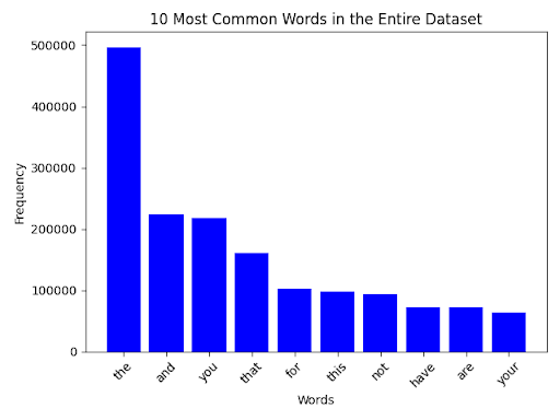
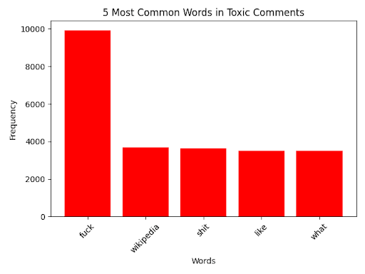
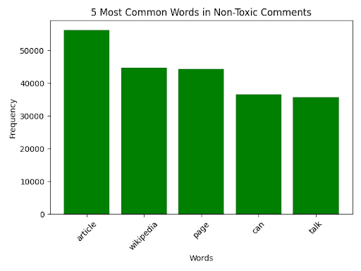
**Fig. 1 |** A graph of the top ten most common words appearing in all comments in the data set.

Figures 1–3 show the top keywords across all comments (Figure 1), toxic-only comments (Figure 2), and non-toxic comments (Figure 3). As expected, toxic comments contained high frequencies of explicit terms such as fuck, shit, and other slurs, whereas non-toxic comments often included words associated with a neutral sense, such as article and talk. Interestingly, certain ambiguous words (e.g. kill) appeared in both classes when looking further down the bar graph, showing how important the role of context is in determining whether a comment should be considered as toxic.

Beyond word frequency’s, the length of the comment also revealed important trends. The dataset ranged from single-word comments to over 200 words, with the majority (about 68%) falling between 5 – 30 words. Toxic comments were slightly shorter on average (~18 words) than non-toxic comments (~24 words), and contained direct insults or short, aggressive phrases. Very short comments (≤10 words) were disproportionately toxic (12.7% toxic vs. 7.8% non-toxic), suggesting that shortness is often associated with toxic remarks. On the other hand, longer comments (>50 words) were more likely to be non-toxic but were one of the biggest causes of false negatives during classification, as they sometimes buried toxic language within the otherwise neutral content. These observations highlight how both word choices and comment length directly influence classification and provide valuable context for evaluating the model’s performance in future iterations.

Model Performance

Evaluating the performance of the BiLSTM model requires careful consideration of the right metrics, particularly because of the dataset’s class imbalance where non-toxic comments make up 90% of the data and toxic comments only 10%. In such significantly imbalanced scenarios, traditional accuracy metrics can be misleading and fail to capture the model’s true effectiveness in classifying toxic comments. Before examining the model’s performance, it is important to understand why accuracy is not the best metric for this classification task. In a dataset where 90% of comments are non-toxic, a naive classifier that simply predicts “non-toxic” for every single comment, without learning any patterns about toxic language whatsoever. This model would still achieve 90% accuracy. This demonstrates why accuracy alone provides such a little insight into a model’s ability to detect the minority class (toxic comments), which is the biggest goal for any content moderation systems.

Given these considerations, the model’s performance is best evaluated through metrics specifically designed for imbalanced classification problems like the one we are dealing with:

F1-Score (63.6%): The F1-score provides the most meaningful single performance indicator for this task, as it harmonically balances precision and recall into a single metric. The achieved F1-score of 63.6% demonstrates that the model maintains reasonable balanced performance in identifying toxic content while accounting for both false positives and false negatives. This metric is particularly valuable because it penalizes models that achieve high recall at the expense of precision, or vice versa.
Recall/True Positive Rate (77.7%): The model successfully identified 11,883 out of 15,294 total toxic comments present in the test set, achieving a recall of 77.7%. This high recall rate is particularly critical for content moderation applications, as it indicates the model successfully catches approximately 4 out of every 5 toxic comments that users post. From a harm prevention perspective, this recall rate represents substantial protection for online communities, as most of the harmful content would be flagged for review or removal.
Precision (54.1%): When the model flags a comment as toxic, it makes the correct classification 54.1% of the time. While this precision presents notable challenges for real-world deployment due to the significant number of false positives it generates, it still represents meaningful pattern recognition that goes far beyond random classification. The precision indicates that the model has learned to identify linguistic patterns associated with toxicity, though it tends to be overly sensitive to certain features.

Figure 4 gives the detailed breakdown of model predictions across all categories, providing insight into the specific types of errors the model makes:

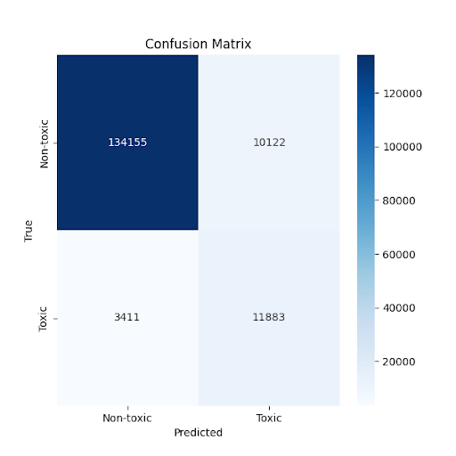
**Fig. 4 |** Confusion matrix showing the distribution of true positives, false negatives, true negatives, and false positives for toxic vs. non-toxic classifications

The confusion matrix reveals the following patterns: True Positives (11,883) represent comments correctly identified as toxic, showing successful detection of harmful content. False Negatives (3,411) are toxic comments that the model failed to identify, representing missed opportunities to flag harmful content. True Negatives (134,155) show non-toxic comments correctly classified as benign, indicating the model’s ability to avoid flagging appropriate content. False Positives (10,112) are non-toxic comments incorrectly flagged as toxic, representing over-moderation. The model achieved an overall accuracy of 70.3%, but this metric requires careful interpretation given the severe class imbalance in the dataset. When carefully examining the accuracy of 70.3%, it comes out that this number reflects the models sophisticated ability to detect toxic patterns in the minority class, but at the cost of some classification errors on the majority class. This illustrates accuracy alone is not only insufficient but can be actively misleading when evaluating classifier performance on imbalanced datasets. While the model shows promise, several limitations must be acknowledged for transparent evaluation. However, the precision score of 54.1% indicates a significant limitation for real-world deployment. This low precision means that approximately 46% of comments flagged as toxic are non-toxic, which could result in a great number of false positives in practical applications. Additionally, the model’s false negative rate of 22.3% means it missed 3,411 toxic comments out of 15,294 total toxic instances, representing harmful content that could continue to cause harassment and create unsafe environments for users if left unaddressed.

To better understand how the binary model performed across the original six toxicity categories, I conducted a post hoc analysis of true positives and false negatives within each class label (toxic, severe_toxic, obscene, threat, insult, and identity_hate). Although the model was trained only to tell toxic apart from non-toxic comments, this breakdown helps to clearly show which types of toxicity were more likely to be correctly identified and which were more overlooked the most. A visual representation of the post hoc analysis for each category is shown in Figure 5.

**Fig. 5 |** True positives (green) and false negatives (red) across the original categories.

As Figure 5 shows, the model has a strong detection on the general toxic class, with most of those comments correctly flagged. However, when we look at the individual categories such as insult, obscene, and identity_hate, the model has showed a proportionally higher false negative rate. This analysis indicates that the binary classifier frequently misclassified these more specific or context-dependent forms of toxicity as non-toxic, proving that identity-related biases can affect detection accuracy across different demographic groups¹⁵. The threat category, which was rare in the dataset, also has notable errors due to limited representation during training. This analysis underscores a limitation of binarization: collapsing multiple distinct toxic categories into a single class can hide performance imbalance across subcategories and implying the need for future work in multi-label classification to more effectively capture the nuances of harmful online discourse.

Traditional Approach vs BiLSTM/RNN Approach

This study identified toxic comments using a Bidirectional Long Short-Term Memory (BiLSTM) Recurrent Neural Network (RNN). To evaluate the effectiveness of this approach, I also implemented a comparison with traditional methods by creating a baseline model using Term Frequency-Inverse Document Frequency (TF-IDF) vectorization combined with a Multinomial Naïve Bayes classifier on the same preprocessed dataset. The baseline model used identical text preprocessing steps (cleaning and tokenization) as the BiLSTM model, and a TF-IDF vectorization with a maximum of 10,000 features. Both models were trained and evaluated on the same train-test split to achieve a fair comparison.

The biggest difference between these approaches is how they process and understand the text they are given. Traditional text processing methods like Bag-of-Words (BoW) and TF-IDF handle text by focusing on word frequency without considering word order or context. Thus, these methods often fail to capture the gentler versions of toxic language, such as sarcasm or implicit threats, and require much more manual interruptions to maintain accuracy. They also perform poorly on longer texts, missing the bigger contextual picture and misclassifying the comments.

In contrast, the BiLSTM model’s ability to understand long-range dependencies is key for accurately identifying toxic language in longer comments. Unlike regular RNNs, which can be very forgetful, LSTMs have special gates—input, forget, and output—that keep track of the information to retain over time. The BiLSTM architecture processes text in both forward and backward directions, capturing context from past and future tokens simultaneously. Additionally, the model uses pre-trained GloVe word embeddings to represent words with vectors carrying semantic meaning, allowing it to start with useful word representations that capture the deeper relationships between words. This comparison is shown in Table 3.

Model	Accuracy	Precision	Recall	F1-Score
TF-IDF + Naïve Bayes	65.4%	51.7%	52.2%	56.6%
BiLSTM + GloVe	70.3% ± 1.2%	54.1% ± 2.0%	77.7% ± 1.5%	63.6% ± 1.7%

Table 3 | Performance comparison between BiLSTM + GloVe and TF-IDF + Naïve Bayes models.

The comparison shows the advantages of the deep learning approach. The BiLSTM model achieved a true positive rate of approximately 78%, a precision of about 54%, and an F1-score of 64% (calculated from TP=11,883; FP=10,112; FN=3,411). The direct comparison on identical data demonstrates that the BiLSTM model achieved better performance across all key metrics, with a 4.9 percentage point improvement in accuracy and a 25.5 percentage point improvement in recall compared to the traditional TF-IDF approach. The F1-score improvement of 7.0 percentage points means the model has a better overall balanced performance. These results confirm the advantages of deep learning approaches over traditional methods for toxic comment classification, looking at earlier studies that reported true positive rates around 60%¹² and 65%¹⁴using traditional approaches. Other hybrid models, such as convolutional and GRU-based architectures¹⁶, show promise and further support the effectiveness of BiLSTM models for toxic comment classification across different languages and contexts¹⁷.

Discussion

The results of this study show that using BiLSTM networks combined with GloVe embeddings greatly improves the classification of toxic comments compared to traditional machine learning methods. The model achieved about 70% accuracy and a true positive rate of 78%, which is better than earlier methods that usually reached true positive rates between 60 and 65 percent. This shows that deep learning is powerful in capturing the complex and subtle features of toxic language. The BiLSTM’s ability to read text in both forward and backward directions help it understand the context around each word, unlike simpler methods such as bag-of-words that ignore word order and meaning. Using pre-trained GloVe embeddings also helps the model generalize better by representing the meaning of words, allowing it to detect toxic comments even when offensive language is hidden with synonyms or different phrasing. The analysis of word frequencies confirmed that toxic comments often contain more rude and insulting words, which supports how the model focuses on these patterns.

The dataset had a class imbalance, with about 90% non-toxic and 10% toxic comments, reflecting real social media content. Simplifying the problem to a binary classification helped the model focus on the main task of finding harmful content. While an F1-score of 63.6% gives a balanced view of performance given the class imbalance, this score is relatively low and shows significant limitations that would need to be addressed before any practical implementation. More importantly, the precision of only 54.1% presents substantial challenges that make the current model unsuitable for real-world deployment without further improvements. This low precision means that nearly half of all comments flagged as toxic would be non-toxic, creating vital over-moderation issues that could upset users trust and platform usability in any production environment. To address these precision limitations in future versions, several strategies could be explored: (1) adjusting the classification threshold to improve the precision-recall trade-off based on specific requirements, (2) investigating alternative loss functions such as focal loss to better handle class imbalance while improving precision, (3) or using ensemble methods or post-processing techniques to reduce false positives. These improvements would be essential for getting from a research prototype to a production-ready system.

Additionally, the model still missed 3,411 toxic comments, which is an important limitation because those harmful comments could still cause damage if not caught. Also, cleaning steps that removed punctuation and capitalization may have reduced the model’s ability to detect tone or sarcasm. The choice to use only two classes may also oversimplify the range of toxic language, missing some important differences in severity or type¹⁸. These issues highlight why human review and further improvements are needed to make detection more reliable. Another limitation of this study arises from part where I simplified the original six toxicity categories into a single binary label (toxic vs. non-toxic)¹⁹. While this made training more computationally practical, it also removed the differences between qualitatively different forms of harm, such as threats, insults, or identity-based hate speech. Removing these categories can weaken the language patterns the model needs to tell different types of toxic comments apart from each other. For example, missing a direct threat is far more serious than missing a generic insult, yet the model treats them both as equally toxic due to the binary framework. Future work should therefore evaluate errors with respect to the original categories to better understand per-class weaknesses and guide improvements toward multi-label or hierarchical classification approaches²⁰.

The imbalanced distribution of toxic vs. non-toxic comments was a strong influencer when it comes to model behavior¹³, contributing to the relatively high recall but lower precision. Future iterations could explore strategies such as class weighting or oversampling methods²¹ (e.g., SMOTE) to address the issue that arises due to this imbalance. Implementing these approaches may reduce the observed number false positives and improve overall precision without sacrificing the recall reported by the model¹⁵.

Compared to newer, more complex transformer models, the BiLSTM model offers a good balance between accuracy and efficiency. This efficiency could potentially make BiLSTM approaches worth looking into for environments with limited recourses, though additional development would be needed for any practical use. Although transformer models might reach higher accuracy, BiLSTM models need less computing power and are easier to run. Future work could explore combining BiLSTM with transformer models to improve understanding of context and robustness²². Developing better ways to measure real-world impact of errors and using techniques that capture emotional tone and story structure could also help improve results.

Besides technical results, automatic toxic comment detection raises important ethical questions. These include concerns about bias, fairness, freedom of speech, and understanding cultural differences. It is important to develop these models openly, regularly check for bias, and always include human moderators to make sure decisions are fair and reasonable, particularly when dealing with identity-related terms that may introduce systematic biases²³. Future automated systems could potentially help classify large amounts of content quickly, but they would still require human oversight for final decisions in complex cases²⁴.Overall, this study aims to provide insights toward developing tools that could eventually support safer and more respectful online communities. The results show that the BiLSTM model improves classification when compared to traditional methods, achieving about 70% accuracy and a true positive rate of 78%. However, a notable limitation of the model is that it missed 3,411 toxic comments (false negatives). If ever the model were to be used in a real-world application this is an issue that should be placed at the highest priority. This shows that while the BiLSTM model does shows promise, it cannot fully replace human moderation or guarantee complete safety. I believe that keeping the internet, a positive place is a responsibility that goes further that this research and should be a priority for everyone involved in an online environment. Future versions should aim to reduce both false positives and false negatives while maintaining model efficiency for the best results.

Acknowledgements

I would like to thank my mentor, Dr.Nived Chebrolu for teaching me the topics that made this project possible and for helping me come up with the idea for this paper.

I also want to thank the Cambridge Center for International Research, where I took summer courses that introduced me to machine learning and natural language processing. The program helped me build the skills I needed to complete this project.

References

S. J. Dixon. Biggest social media platforms by users 2025. Statista. https://www.statista.com/statistics/272014/global-social-networks-ranked-by-number-of-users/ (2024). [↩]
S. Hinduja, J. W. Patchin. Cyberbullying: 2020 edition – Identification, prevention, and response. Cyberbullying Research Center. https://cyberbullying.org/Cyberbullying-Identification-Prevention-Response-2020.pdf (2020). [↩]
Jahan, M. S., and M. Oussala. “A Systematic Review of Hate Speech Automatic Detection Using Deep Learning.” Neurocomputing, 2023. [↩]
Raza, S., et al. “HarmonyNet: Navigating Hate Speech Detection.” ScienceDirect, 2024. [↩]
Elsafoury, F. “Investigating the Impact of Bias in NLP Models on Hate Speech Detection.” ACL Anthology, 2023. [↩]
Khan, M. A., and M. A. Khan. “Determination of Toxic Comments and Unintended Model Biases.” arXiv, 2023. [↩]
A. Joulin, E. Grave, P. Bojanowski, T. Mikolov. Bag of tricks for efficient text classification. arXiv preprint arXiv:1607.01759 (2016). [↩]
Zampieri, Marcos; Shervin Malmasi; Preslav Nakov; Sara Rosenthal; Noura Farra; Ritesh Kumar. “SemEval-2019 Task 6: Identifying and Categorizing Offensive Language in Social Media (OffensEval).” arXiv, 19 Mar. 2019, arXiv:1903.08983 [↩]
J. Pennington, R. Socher, C. D. Manning. Glove: Global vectors for word representation. Proc. Conf. Empirical Methods in Natural Language Processing. 1532–1543 (2014). [↩]
D. P. Kingma, J. Ba. Adam: A method for stochastic optimization. arXiv preprint arXiv:1412.6980 (2014). [↩]
Dessì, Danilo; Reforgiato Recupero, Diego; Sack, Harald. “An Assessment of Deep Learning Models and Word Embeddings for Toxicity Detection within Online Textual Comments.” Electronics, vol. 10, no. 7, 2021, article 779, DOI:10.3390/electronics10070779. [↩]
T.Davidson, D. Warmsley, M. Macy, I. Weber. Automated hate speech detection and the problem of offensive language. Proc. Int. AAAI Conf. Web Soc. Media. 11, 512–515, 2017. [↩] [↩]
Garg, Tanmay; Sarah Masud; Tharun Suresh; Tanmoy Chakraborty. “Handling Bias in Toxic Speech Detection: A Survey.” arXiv, 26 Jan. 2022, arXiv:2202.00126. [↩] [↩]
P. Badjatiya, S. Gupta, M. Gupta, V. Varma. Deep learning for hate speech detection in tweets. Proc. 26th Int. Conf. World Wide Web Companion. 759–760 (2017). [↩] [↩]
Vaidya, Ameya; Feng Mai; Yue Ning. “Empirical Analysis of Multi-Task Learning for Reducing Model Bias in Toxic Comment Detection.” arXiv, 21 Sep. 2019, arXiv:2009.09758. [↩] [↩]
Z. Zhang, D. Robinson, J. Tepper. Detecting hate speech on Twitter using a convolution-GRU based deep neural network. In The Semantic Web. ESWC 2018, Lecture Notes in Computer Science, vol 10843. Springer, Cham, 706–720 (2018). [↩]
Khan, Shahzad; Malik, etc. “Indonesian Hate Speech Detection Using IndoBERTweet and BiLSTM.” Journal of Open Innovation: Technology, Market, and Complexity, [vol./issue as per source], 2023. [↩]
S. Karlekar, M. Bansal. SafeCity: Understanding diverse forms of sexual harassment personal stories. Proc. Conf. Empirical Methods in Natural Language Processing. 2805–2811 (2018). [↩]
Bhatti, Faisal, et al. “Deep learning for religious and continent-based toxic content detection and classification.” PMC-NCBI, 2022, DOI as per source. [↩]
Ahmed Belal, Tanveer, G. M. Shahariar, Md. Hasanul Kabir, et al. “Interpretable Multi Labeled Bengali Toxic Comments Classification using Deep Learning.” arXiv, 8 Apr. 2023, arXiv:2304.04087. [↩]
Zhou, Fang; Hanlu Zhang; Jacky He; Zhen Qi; Hongye Zheng. “Semantic and Contextual Modeling for Malicious Comment Detection with BERT-BiLSTM.” arXiv, 14 Mar. 2025, arXiv:2503.11084. [↩]
Shinde, Ashish, Pranav Shankar, Atul Atul, and Srikari Rallabandi. “Bidirectional LSTM with Convolution for Toxic Comment Classification.” Proceedings of the 1st International Conference on Artificial Intelligence, Communication, IoT, Data Engineering and Security (IACIDS 2023), Lavasa, India, EAI, 2024, DOI:10.4108/eai.23-11-2023.2343140. [↩]
Van Dorpe, Josiane; Zachary Yang; Nicolas Grenon-Godbout; Grégoire Winterstein. “Unveiling Identity Biases in Toxicity Detection: A Game-Focused Dataset and Reactivity Analysis Approach.” Proceedings of the 2023 Conference on Empirical Methods in Natural Language Processing – Industry Track, 2023, pp. 263-274. [↩]
Park, J. H.; J. Shin; P. Fung. “SS-BERT: Mitigating Identity Term Bias in Toxic Comments Classification by Utilising the Notion of ‘Subjectivity’ and ‘Identity Terms’.” Preprint submitted 6 Sept. 2021. [↩]

Binary Toxic Comment Classification Using BiLSTM and GloVe Embeddings

Abstract

Introduction