A Modern Approach to Uplift Marketing: Using Artificial Intelligence to Maximize Marketing Efficiency

The digitalization of marketing has shifted focus from broad, mass-market campaigns to highly personalized, data-driven approaches. In this shift, uplift modeling emerged to provide a causal framework for estimating the incremental effect of marketing developments, allowing for more efficient strategy. This study investigates the practicality of predicting exposure, an essential precursor to customer response. Using the CRITEO-UPLIFT dataset of over 25 million data points, we evaluate both single-model and two-model approaches, employing Random Forest, XGBoost, and neural networks to predict exposure based on anonymized features and treatment assignments. Severe class imbalance in exposure was addressed through undersampling, oversampling through SMOTE-uplift, and class-weight adjustments, with hyperparameter tuning performed using grid search and hyperband optimization. Model evaluation incorporated traditional metrics (precision, recall, F1, AUC) and uplift-specific metrics (AUUC, Qini coefficient). Results showed that models trained on imbalanced data underperformed in detecting exposed individuals, with very low recall and F1 scores, while resampling, particularly undersampling, substantially improved predictive stability and uplift gains. Among the tested methods, XGBoost and neural networks demonstrated superior scalability and efficiency, while Random Forests offered interpretability advantages. Feature importance analysis using SHAP values highlighted nuanced, non-linear interactions across variables, reinforcing exposure as a critical determinant in uplift analysis. Overall, this study demonstrates that machine learning can effectively predict exposure, enabling businesses to allocate marketing resources more efficiently and enhance causal inference in campaign evaluation.

Keywords:   

Uplift modeling, CRITEO-UPLIFT dataset, machine learning, exposure prediction, class imbalance, causal inference, marketing analytics

Introduction

With the digitalization of the world, the concept of business and marketing as a whole has taken a complete upheaval. Once reliant on mass broadcast, marketing has become data-driven and highly personalized. One of the most impacted areas is that of marketing, in which businesses have come to rely extensively on real‑time consumer analytics and CRM platforms. Considering the importance of marketing in all aspects of business, the applications of the following findings will be able to allow for more efficient marketing techniques and demographic targeting. Marketing is such an important department, that with the data, companies could save large percentages of their budget, exposing their products to those who would most likely become a customer.

In 2023, large technology corporations such as Alphabet and Microsoft spent on average around 9.1% of their total revenue on marketing, with total global spending on marketing being upwards of $1T¹. While noting these statistics, the importance of marketing must be noted. This marketing budget incorporates numerous different methods and channels however, including promotional media, direct selling, and business to business (B2B) selling by allocating budget to purchasing social media advertisements, consumer relationship management (CRM) systems to gather marketing data, and promotional events. While a large portion of this budget is not directed towards specifically advertising to the mass market, the sheer size of the marketing budget implies that any small deviation may save a business a massive amount of potential profits.

When taking a look at the marketing industry itself, a reasonable definition of its responsibilities, costs and trends is useful to understand the impact of making the process more efficient. First, the responsibilities of the marketing department mainly consist of controlling the company’s brand, values, and public vision. This is completed primarily through marketing campaigns, public messaging, and public relations. In addition to this, the marketing department handles data regarding the performance of the company’s products, gathers consumer data, as well as market data. Through these activities, the marketing department is able to have a holistic view of the company’s circumstances and is the liaison between the organization and the consumers. As demonstrated, the marketing division is extremely important to every company’s operations, and a more cost and time efficient department would greatly improve overall performance. The costs of the marketing department are primarily set in its content creation costs, market research costs, and publishing costs. Uplift marketing, the core of this study, is focused towards diminishing market research costs.

Currently, the most commonly used marketing strategy is targeted marketing, which utilizes customer data to specifically market to a specific customer demographic. Standard ‘targeted’ marketing models typically estimate purchase likelihood, whereas uplift marketing (a form of Conditional Average Treatment Effect (CATE) modeling) instead estimates the incremental effect of treatment (), providing a truly causal, quantitative measure of campaign impact². Early conceptual work such as by Radcliffe formalized the idea of ‘True-Lift’ targeting, which explicitly models the incremental impact of interventions compared to control groups³. Optimizing uplift models thus enables more precise estimates of incremental lift, empowering firms to allocate budget on the individuals most likely to respond.

Previous authors examining the CRITEO-UPLIFT dataset have also found the data to be an interesting study in the field of uplift marketing prediction and data analysis. Looking at the dataset, the columns include different hidden feature values (hidden for participant privacy), treatment, visit, exposure, and conversion⁴. The feature values each describe an aspect of each data value, treatment separated the control group from the treatment group (marketing effectively applied), visit describes whether or not this data value visited a physical or digital store, exposure refers to whether or not the data value was exposed to marketing, and finally conversion refers to whether or not the data value became a loyal customer. These authors have analyzed the viability of utilizing the dataset in practical settings while analyzing the distribution of data through graphs and models such as with measuring model separability⁵. The large problem which all papers note regarding the paper is the imbalance in data with the vast majority of data on those who did not ultimately purchase a product and those who have. Some specific methods which were utilized to address this issue included the modification of the initial dataset using a class of synthetic response surfaces to create a semi-synthetic version of the dataset⁶. In addition, a Classifier Two-Sample Hypothesis test was used to test treatment predictability and improvement of the new dataset’s prediction accuracy for visits and conversion, which revealed the model constructed had more success than a random classifier and that features were useful for any models created. In addition, the study found that after a sample size of 1 million, different approaches to the data would yield more separate results, meaning that having a massive dataset would indeed be useful. For this particular dataset, through AUUC performances compared to existing datasets, the study proved that the large size of the CRITEO-UPLIFT dataset was in fact productive. As the test data size increased, the AUUC score for all uplift models tested would increase at an almost proportional rate after 50 thousand test data size and up to the maximum 2.8 million test data size.

Previous work on the CRITEO-UPLIFT dataset has employed statistical methods such as logistic regression, propensity score matching, and hypothesis testing to analyze uplift modeling and estimate causal effects. In parallel, deep learning methods have been adapted for uplift modeling. Belbahri et al. proposed neural networks that jointly optimize transformed outcomes and mean difference losses⁷. More recent advances embed causal representations within graph neural networks use dual estimators to address label scarcity⁸’⁹. These approaches primarily focused on assessing treatment effects by comparing outcome distributions across treatment and control groups. Hypothesis testing, including t-tests and chi-square tests, have been used to determine the statistical significance of observed differences. However, these methods have limitations, including sensitivity to model misspecification, difficulties in handling data, and challenges in capturing complex, non-linear relationships between features and treatment effects. Additionally, standard hypothesis testing often assumes independence and homogeneity of treatment effects, which may not hold in real-world scenarios, leading to unreliable estimates.

Another study by Xu et al. 2022, was through the use of neural networks, more specifically, a neural uplift model focused on transforming raw data into more abstract representations and overall simplifying them to increase interpretability. Ultimately, this study demonstrated that attentive neural network models (ANU) achieve better performance than previously considered models such as Promoted Cumulative Gain (PCG) and X-learner, with the highest AUUC scores across all datasets (Hillstrom, Criteo, Zenodo), being the ANU model with AUUC scores of 0.3072, 0.01514, and 0.10591 respectively (this is not accounting for standard error values). Beyond specialized uplift architectures, general-purpose meta-learners such as the X-Learner provide flexible strategies for estimating heterogeneous treatment effects, making them broadly applicable to uplift tasks¹⁰. More recently, meta-learner frameworks such as R-Learner¹¹ have expanded uplift modeling by providing flexible, model-agnostic strategies for estimating heterogeneous treatment effects. Complementary work has combined causal forests with deep reinforcement learning to dynamically optimize interventions¹².

When looking at the previously conducted studies, we note that numerous different approaches have been taken, however while many studies have examined the effect of treatment or attempted to predict visit/conversion, exposure has never been the specific focus of any previous study on this dataset. Exposure, being the core of uplift marketing itself, is the necessary precursor to any causal treatment effect, and modeling it reduces bias from non-compliance between treatment assignment and actual reach. As Lo et al. notes, uplift modeling’s value lies in finding persuadable individuals whose behavior changes only if they are reached, making exposure the most practical and effective target¹³.

Based on these considerations, this study seeks to answer the following research question:
How accurately can machine learning models predict which individuals are most likely to be effectively exposed to marketing treatments using the CRITEO-UPLIFT dataset? In the process, as shown by Figure 1, we will evaluate different approaches and the models to accurately predict, based on the features of a subject, the probability that they will be effectively exposed, essentially conducting uplift marketing analysis through machine learning methods. By doing so, we hope to approach uplift marketing through the new lens of machine learning so that businesses can more easily market to potential customers. The research deliberately focuses on methodological advances within the established uplift modeling framework, applying technological advances to improve upon traditional target marketing methods. Through the usage of more flexible models, we can deliver quantifiable improvements in causal uplift prediction, measurements that can be benchmarked against existing baselines.  

Dataset

In this study, we used the CRITEO-UPLIFT dataset, a comprehensive dataset with over 25M entries encapsulating different aspects of uplift marketing built utilizing multiple incrementality tests, a randomized trial procedure where a random sample from the population is prevented from being targeted by advertising¹⁴.

In total, the dataset holds 16 columns, with 12 of them being feature values, and the other 4 being treatment, conversion, visit, and exposure, respectively. More specifically, treatment records whether or not the subject has received the marketing, conversion records whether or not the subject has been converted to a user/customer, visit records whether or not the subject has conducted a visit (to the store or service), and exposure records whether or not the subject has been effectively exposed. The feature values themselves are hidden deliberately by CRITEO, the creators of the dataset to protect the identities of the subjects included in the dataset.

Before proceeding to exploratory analysis, we briefly state the causal identification assumptions that justify interpreting differences in recorded exposure as causal effects. We frame inference in the potential-outcomes paradigm¹⁵, which requires three identifying conditions: unconfoundedness (no unmeasured confounders given observed covariates), SUTVA (no interference and consistent treatment definition), and overlap (sufficient common support between arms). CRITEO’s randomized design makes unconfoundedness plausible in expectation, but real-world issues, non-compliance/delivery failures, very low recorded exposure relative to treatment, and possible spillovers, limit identification in parts of the covariate space. For these reasons we model actual recorded exposure to reduce bias from non-compliance, report balance and overlap diagnostics in Methods, and interpret estimated differences in exposure cautiously as suggestive causal lift under the assumptions above.

Exploratory Data Analysis  

In this section, an exploratory data analysis of the CRITEO-UPLIFT dataset is presented, in which we will explore and present any patterns, trends, or relationships discovered. This will be completed through the visualization of highlighted sections, as well as looking at the data through multiple perspectives. In doing so, an understanding of the dataset as well as any challenges will be faced later during the experimentation process.

Figure 2 illustrates how many of the subjects have been exposed, with those labeled with a 0 being unexposed, and those with a 1 being considered as exposed. When taking a closer look at the actual distributions, around 13.5 million data values are considered to be unexposed, and only 400 thousand data values are actually exposed. In percentages, approximately 96.9% of the data values were unexposed, while around 3.1% of the data values were exposed. The massive data imbalance poses the large issue of model bias, affecting accuracy of the model in the process. Although this data imbalance is startling, considering the size of the dataset, the minority class will still have 400 thousand data values.

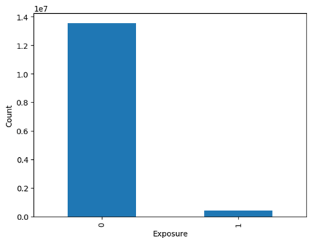
Figure 3 demonstrates the data imbalance in the target variable but relative to whether or not the data value is treated (denoted by a value of 1) or not (denoted by a value of 0). We note a similar decrease in counts from data values which are exposed vs. those which aren’t exposed. When taking a look at the specific statistics, around 400 thousand data values were treated and exposed, 11.4 million data values were treated but not exposed, not a single data value was exposed and not treated, and around 2.1 million data values were neither treated nor exposed. When converted to percentages, 3.06% of data values were both treated and exposed, 81.94% were treated and not exposed, and 15% were neither treated nor exposed.

Next, we explored descriptive statistics of other 12 features in our datasets. Table 1 describes the statistics of each feature in the dataset. To begin, the mean of each variable is where the vast majority of data values encapsulated in that variable are located, as the majority of variables being concentrated in a small proximity. This results in the interquartile means being extremely close to each other in the majority of values, accompanied by a large jump to the maximum value, as a result of outliers. The only exceptions to this are f0 and f6, with a wider distribution of overall values. In addition, the standard deviations (std) of each variables explains either the wider distribution of data values or a small concentration of extreme outliers, such as with f9.

	Count	Mean	Std	Min	25%	50%	75%	Max
f0	13979592.0	19.620297	5.377464	12.616365	12.616365	21.923413	24.346459	26.745255
f1	13979592.0	10.069977	0.104756	10.059654	10.059654	10.059654	10.059654	16.344187
f2	13979592.0	8.446582	0.299316	8.214383	8.214383	8.214383	8.723335	9.051962
f3	13979592.0	4.178923	1.336645	8.398387	4.679882	4.679882	4.679882	4.679882
f4	13979592.0	10.338837	0.343308	10.280525	10.280525	10.280525	10.280525	21.123468
f5	13979592.0	4.028513	0.431097	9.011892	4.115453	4.115453	4.115453	4.115443
f6	13979592.0	4.155356	4.577914	31.429784	6.699271	2.411145	0.294443	0.294443
f7	13979592.0	1.105716	1.025248	4.883815	4.838315	4.838315	4.838315	4.838315
f8	13979592.0	3.933581	0.156660	3.633457	3.910792	3.971858	3.971858	3.971858
f9	13979592.0	10.267638	7.018975	13.190056	13.190056	13.190056	13.190056	75.297507
f10	13979592.0	5.333396	0.168229	5.300375	5.300375	5.300375	5.300375	6.473917
f11	13979592.0	0.170967	0.022833	1.383941	0.168679	0.168679	0.168679	0.168679
treatment	13979592.0	0.850000	0.357071	1.000000	1.000000	1.000000	1.000000	1.000000
exposure	13979592.0	0.030631	0.172316	0.000000	0.000000	0.000000	0.000000	1.000000

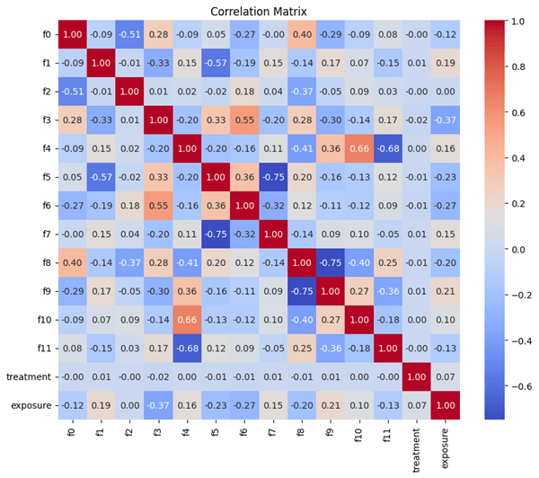
To understand the relationships between the variables, we computed the Pearson’s correlation coefficient between the variables as shown in Figure 4. A perfectly positive correlation (both variables are perfectly linearly related) occurs at a correlation value of 1, while a perfectly negative correlation (both variables are perfectly inversely related) at -1. We note that there is an extremely low coefficient value between treatment and any other variable in the dataset. However, we observed two relatively highly correlated feature pairs such as with f8 and f9 (-0.75), f5 and f7 pairs (-0.75). Although the correlation coefficients are relatively high, they do not cross the threshold of +/- 0.8 which we deemed to be an implication of collinearity. When taking a look at the target variable of the model, no variables were particularly high when correlated, with the highest values being f3 at -0.37 and f6 at -0.27.

Methods and Models

Input Feature and Output Target

This investigation’s primary approach was to input the original features (12 anonymized features and treatment) given in the dataset. The output target is exposure, due to the purpose of uplift marketing being identifying those who are the most likely to respond to exposure, namely whether or not these individuals are effectively exposed, rather than their consequent actions. This would mean that we would mostly ignore the visit and conversion variables to understand the effect of treatment and the 12 feature values on exposure only.

While conversion is often considered the ultimate marketing goal, exposure was selected as the target variable in this study due to both strategic and methodological considerations. Compared to conversion, which is significantly more imbalanced and influenced by various external factors like product pricing, personal interest, or market conditions, exposure provides a more causally linked outcome to model in uplift marketing. By predicting which individuals are most likely to be effectively exposed, businesses can allocate resources more efficiently and predictably increase the likelihood of conversions. This focus aligns with the goal of uplift marketing: not simply to predict who will buy, but to identify who is most likely to respond positively to marketing efforts. Additionally, exposure allows for more stable model performance given the larger positive sample size compared to conversion, making it a more viable target for statistical and machine learning techniques.

Single Model Approach

In the single model approach, a machine learning model is trained and tested using a unified dataset, including the 12 feature and treatment variable. Through this training, the model learns the underlying patterns between the unified dataset and the target outcome—exposure. This approach offers a simple yet effective framework for estimating the likelihood of exposure while accounting for both feature data and treatment status within a single predictive model.

Models

For the model development, the dataset was split into train and test sections with 30% of the data being allocated to the test section and 70% of the data allocated to the train section with a stratified split to retain the class proportion of the dataset in both sections. A 30/70 split was chosen for the model because of the high volume of data in the dataset, allowing for more data to test for accuracy while still retaining enough to ensure the highest accuracy model given the data.

We primarily chose random forest and XGBoost models for the purposes of this experiment due to it being the most time efficient model considering the size of our dataset. In addition to this, neural networks were applied due to its flexibility and scalability with large datasets. The random forest model is an algorithm which creates decision trees and trains each tree on a random piece of training data with a random subset of features¹⁶. After doing so, the model outputs the either the mean or the mode of the predictions depending on whether or not the model is focus on regression or classification.  The purpose of random selection is the reduction of overfitting, which was a concern for this dataset. The advantages of such a model are its resistance to outliers, handling of imbalance data, and handling of high feature datasets.

XGBoost, or Extreme Gradient Boosting, is an algorithm which creates trees sequentially while repeatedly changing the model’s parameters to adapt to errors in previous trees¹⁷. In the process, the algorithm also calculates the importance of each tree to reducing the error in the model and give them importance values in accordance with their contribution. This process continues until additional trees no longer significantly reduce the objective function, or how well the model predicts the target variable. What differentiates XGBoost from traditional gradient boosting models is the inclusion of regularization elements to prevent overfitting. Advantages of XGBoost models include faster training, more refined feature importance control, and extremely good regularization control. Something that makes XGBoost particularly excels at is processing speed, which is achieved through parallel processing, which becomes especially noticeable on large datasets. This is particularly useful considering the size of the dataset, requiring fast processing in order to make the model practical in handling practical applications.

Neural networks are a specific class of machine learning algorithms consisting of layers of interconnected nodes, or “neurons,” that process data by learning patterns through a system of weights and biases adjusted during training¹⁸. Each layer captures complex relationships and interactions in the data. The training process involves forward propagation to generate predictions and backpropagation to update weights based on prediction errors, ending when the loss function has been minimized. Advantages of neural networks include their flexibility and performance on unstructured data. One particular strength of neural networks lies in their ability to be trained efficiently on very large datasets, making it extremely useful in the context of the CRITEO-UPLIFT dataset.

Evaluation Metrics

The evaluation of model performance relies on several metrics. Precision, recall, and F1 score are applied to both train and test datasets in order to capture the balance between correctly identifying exposed individuals and avoiding false positives. Log-loss is reported to assess probabilistic calibration and model stability across folds. Standard classification benchmarks such as the Area Under the ROC Curve (AUC) provide a measure of separability. For uplift-specific evaluation, the Area Under the Uplift Curve (AUUC) and the Qini coefficient are employed, quantifying uplift. Together, these metrics capture both traditional classification accuracy and the true causal effectiveness of uplift models.

Hyperparameter Tuning

Hyperparameter tuning is the process in which the optimal input parameters into a model is found by inputting numerous combinations and running the model using these respective input parameters. While seemingly inefficient, it is an automatic way of tuning the model through trial and error which provides insight to the impact of various input parameters as well as the outputting the most effective model available within the given combinations. By doing so, the model’s performance could be significantly improved with the correct combination of input parameters. The method chosen for this experiment was grid search, which creates a grid of possible parameter values and inputs every possible combination of these parameters into the model¹⁹. The specific parameters chosen for each model as well as their ranges are illustrated in Table 2.

In our Grid Search process, we performed 5-fold cross-validation to address potential concerns regarding model stability and minimize overfitting, while using the weighted f1-score to account for class imbalances²⁰. The mean and standard deviation of the log-loss across folds remained highly consistent indicating negligible variance and robust convergence. The model’s held-out test performance closely aligned with the cross-validated estimates. These results demonstrate that the reported metrics are stable across folds and not artifacts of a single 30/70 split. When tuning hyperparameters for random forest models, we focus on n_estimators, max_depth, min_samples_split, max_features, and class_weight to optimize performance. n_estimators determine the total number of trees in the model, and for a large dataset, increasing this value helps capture complex patterns while reducing variance. The input values used for n_estimators range from 100 to 500. Max_depth controls how deep each tree can grow, and limiting it prevents excessive branching that could lead to overfitting. The input values used for Max_depth range from none to 25. Similarly, min_samples_split ensures that nodes only split when enough samples are present, preventing unnecessary complexity in large datasets. The input values used for min_samples_split range from 50 to 150. Additionally, max_features regulate how many features are considered at each split, which helps maintain model diversity while improving efficiency. The input values used for max_features range from 1 to 12. Finally, class_weight is particularly useful for handling class imbalances, ensuring that the model does not disproportionately favor majority classes. The input values used for class_weight range from none to balanced.

For XGBoost, we focus on eta, subsample, colsample_bytree, and scale_pos_weight to balance learning speed and generalization. Eta reduces feature weights after each boosting step, making training more conservative and mitigating overfitting. The input values used for eta range from 0.01 to 0.3. Subsample randomly selects a portion of training data before growing trees, introducing randomness that prevents overfitting while maintaining robustness. The input values used for subsample range from 0.5 to 0.9. Colsample_bytree controls how many features are randomly sampled for each tree, improving efficiency in high-dimensional datasets. The input values used for colsample_bytree range from 0.5 to 0.9. Lastly, scale_pos_weight gives fair weights to minority classes and improving model fairness in unbalanced datasets by doing so. The input values used for scale_pos_weight range from 0.01 to 100.

Hyperparameter tuning of neural networks using the hyperband algorithm was chosen as it allows for efficient optimization by allocating training resources to the most promising model configurations²¹. Hyperparameters chosen include units_0, units_1, and units_2 (fully connected neurons in each layer), activation (activation function), and learning_rate (controls weight updates). The epochs parameter defines the total training duration, while initial_epoch allows training to resume from a specified point. Hyperband organizes trials into brackets and rounds, where each bracket represents a different early-stopping schedule and each round filters out weaker trials. Each model configuration is tracked using a unique trial_id, enabling comparison and reproducibility. The model has 2 hidden dense layers (64 neurons in the first layer and 32 in the second), no dropout layers, runs on a batch size of 32 with Adam optimizer, categorical_crossentropy loss, and a learning rate of 0.001.

Model	Parameters	Description	Ranges
Random Forest	n_estimators	n_estimators determines the total number of trees in the model, and for a large dataset, increasing this value helps capture complex patterns while reducing variance.	[100, 500]
	max_depth	Max_depth controls how deep each tree can grow, and limiting it prevents excessive branching that could lead to overfitting.	[None, 5, 10, 15, 20, 25]
	min_samples_split	Min_samples_split ensures that nodes only split when a sufficient number of samples are present, preventing unnecessary complexity in large datasets.	range(50,150,10)
	max_features	Max_features regulates how many features are considered at each split, which helps maintain model diversity while improving efficiency.	range(1,12,1)
	class_weight	Class_weight is particularly useful for handling class imbalances, ensuring that the model does not disproportionately favor majority classes.	[None, “balanced”]
XGBoost	eta	Eta reduces feature weights after each boosting step, making training more conservative and mitigating overfitting.	[0.01, 0.05, 0.1, 0.2, 0.3]
	subsample	Subsample randomly selects a portion of training data before growing trees, introducing randomness that prevents overfitting while maintaining robustness.	[0.5, 0.6, 0.7, 0.8, 0.9]
	colsample_bynode	Colsample_bytree controls how many features are randomly sampled for each tree, improving efficiency in high-dimensional datasets.	[0.5, 0.6, 0.7, 0.8, 0.9]
	scale_pos_weight	Scale_pos_weight gives fair weights to minority classes and improves model fairness in unbalanced datasets.	[0.01-100]
Neural Network	units_0, units_1	Units_0 and units_1 represent the amount of neurons in the first and second hidden layers respectively.	range(32, 256, 32)
	num_layers	Num_layers represents the total amount of hidden layers.	range(1, 3, 1)
	activation	Activation represents the activation function of the hidden layers.	[“relu”, “tanh”]
	learning_rate	Learning rate controls how quickly the model updates its weights.	range(1e-4, 1e-2)

Two Model Approach

In addition to the single-model approach, a two-model strategy is implemented to estimate individual uplift. This approach involves dividing the dataset into training and testing subsets, then further partitioning only the training data by treatment. two separate training sets are created: the treatment group, containing only data values that received treatment, and the control group, containing only data values who have not received treatment.

Two separate predictive model is trained on each group. both models are with the objective of predicting exposure based on the 12 feature variables, with the only difference being that one model is trained exclusively on the treated subset, and the other being trained exclusively on the no treatment control. Once trained, both models are applied independently on the entire test set. For each data value in the test set, the treated model outputs a predicted probability of exposure if individual had received treatment. Similarly, the control model outputs a predicted probability assuming no treatment. The uplift score for each test instance is then computed as the difference between these two predicted probabilities. This score represents the estimated effect of treatment.

We wish to note that we intentionally restricted the control group to non-treated, non-exposed individuals. This choice creates a cleaner baseline by specifying users who had no marketing exposure, mirroring real-world marketing strategy. Most importantly, this enhances the causal validity of uplift by ensuring observed difference relation.  

To assess the performance of the two-model approach, uplift-specific evaluation metrics are applied, those being the Qini curve and the uplift curve²². The uplift curve plots the cumulative treatment effect as individuals are ranked by their predicted uplift score, visualizing how much incremental gain is achieved. The Qini curve is a related visualization tool that compares the uplift model to a random targeting strategy, showing the added value of using the model for decision-making. From the Qini curve, the Qini coefficient can be calculated as the area between the model’s curve and the baseline area. A larger Qini coefficient indicates that the model more effectively distinguishes individuals who are positively influenced by the treatment from those who are not.

Handling Data Imbalance

When it comes to handling the data imbalance which is present in the dataset, four different approaches were taken: custom loss functions, undersampling, oversampling, or using the original dataset but with balanced weights.

When it comes to custom loss functions we took a look at imbalance-specific methods such as custom loss functions and stratified batch sampling. Custom losses, including class-weighted cross-entropy and focal loss, modify the training objective so that errors on minority-class examples receive greater weight, encouraging the model to pay more attention to exposed users²³. Stratified batch training instead changes the data pipeline by constructing each mini batch with balanced class proportions rather than sampling randomly, aiming to stabilize learning under skewed distributions²⁴. While both approaches produced strong in-sample results, they failed to generalize, indicating overfitting to the rebalanced training distribution rather than genuine gains in uplift performance. Consequently, we excluded these methods from further study.

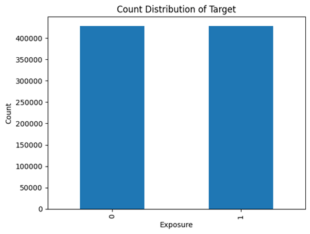
For undersampling, the imbalance with the vast majority of data values not being effectively exposed was randomly undersampled to set the amount of data values which were exposed and unexposed close to equal, as revealed by the large disparity shown in the exploratory data analysis section. The method chosen for undersampling is random undersampling, which randomly deletes data values in the original data set from the majority class as to even out the value counts, a visualization of the results is visualized in Figure 5, where both exposed and unexposed value counts equal approximately 400 thousand. Although undersampling removed ~97% of the 25 M rows, this was necessary given the dataset’s extreme imbalance and redundancy. Alternatives such as cost‑sensitive learning with weighted XGBoost preserved scale but failed to match the uplift gains from undersampling. The discarded examples were largely repetitive majority‑class instances adding little causal signal, while the reduced dataset improved convergence, cut computation, and delivered superior uplift performance. Thus, in terms of this dataset, scale alone, praised in prior Criteo studies, does not outweigh precision.

When oversampling, the amount of exposed data values was synthetically increased to decrease the imbalance between the exposed and unexposed data values.  The method specifically chosen for oversampling is SMOTE-uplift²⁵, standing for synthetic minority oversampling technique designed for uplift modeling. This method creates synthetic data by interpolating through existing datapoints while accounting for treatment/control group dependency. In doing so, new data which does not disrupt any current patterns and instead only inflating the data value counts is created.  Before oversampling, the data contains massive imbalance, but afterwards, an identical amount of data fitting both those exposed and not exposed is created, eliminating data bias in regard to data size. Oversampling is only applied to the train dataset, while data imbalance still exists in the test dataset.

While built in class weights balancing methods of handling data imbalance exist, such as with class_weight in Random Forest which could adjust class importance inversely to frequency and in XGBoost where scale_pos_weight which could increase the weight of the minority class, we aim to compare these built-in methods with resampling techniques to assess their effectiveness without altering original data distribution.

These models will be evaluated using precision, recall, and F1-score, where precision measures false positives, recall assesses true positive detection, and F1-score balances both. By comparing class weights balancing and resampling, we aim to determine which approach best mitigates class imbalance while maintaining model accuracy.

Feature Importance Analysis

Once the optimal model has been found, we aim to explore the nuances of the dataset. More specifically, we wish to explore the contribution of each of the features, including treatment, on model prediction and other variables This will be completed with feature importance analysis.

Feature importance analysis is the process in which the contribution of each feature in a model is found, by which the model could be more efficient by means of inputting only relevant features. In addition to this, the relationships between certain variables could be discovered, yielding potentially key insights for other applications. Tradition feature analysis provides an idea of the contribution of features across all predictions, not providing case specific explanations. Because of this as well as potential introduced biases, we chose to use SHAP values instead.

SHAP, or Shapley Additive exPlanations, is a method based in cooperative game theory²⁶. For each prediction, SHAP values provide an understanding of how much each feature contributed for that specific prediction. It does so through a calculation of all possible combinations of feature, giving a much more accurate picture of the contribution of features for each prediction.  We chose SHAP analysis not only for its advantages in prediction specific details as well as a more accurate analysis overall, but also because it utilizes the same method across all models, while traditional feature analysis has model-specific habits.

Results and Discussion

Single Model Approach Results and Discussion

After tuning and testing the model, results from the original imbalance dataset, an undersampled dataset, and an oversampled dataset were all compiled. To quickly mention, confidence intervals were gathered for each evaluation metric however due to their insignificant size they were not included in the tables themselves.

For the XGBoost model trained on the original imbalanced dataset, model results exhibit clear evidence of overfitting and poor performance. Looking at the results of Table 3, while the F1 scores for those exposed and unexposed are 0.99 for both train and test, exposed data values suffer significantly with an F1 score of only 0.26 in both cases. This poor performance is driven by extremely low recall (0.17 in train and 0.16 in test), indicating that the model is failing to correctly classify many positive instances. Even though precision remains moderate, the inability to recall positive cases results in a heavily biased model that favors label 0. Despite the use of scale_pos_weight to penalize the weights, the model still heavily struggles with class imbalance.

When looking at the Random Forest model trained on the original imbalanced dataset, results indicate similar issues to the xgboost model, namely overfitting and generalization to the positive class. While the model achieves strong performance for the unexposed class (label 0) with F1 scores of 0.97 on the training set and 0.96 on the test set, performance on the exposed class (label 1) is much weaker. On the training set, the F1 score for the exposed class is 0.54, supported by high recall (0.97) but low precision (0.37), suggesting the model is overpredicting positives. However, this performance is not sustained in the test set, where the F1 score drops to 0.37 due to low scores in both precision (0.26) and recall (0.65). This drop highlights the model’s struggle to accurately classify minority class instances, reflecting the persistent impact of class imbalance.

The neural network, on the other hand, achieved high performance on class 0, with precision, recall, and F1-scores all achieving around 0.91–0.99 on both training and test sets. In contrast, results for class 1 were significantly lower, with an F1-score of just 0.25, indicating poor classification for that class and severe aftereffects of class imbalance.

Models	Train/ Test	Label (Exposed)	Precision	Recall	F1	Samples
Random Forest ‘max_features’=12, ‘min_samples_split’ = 50, ‘n_estimators’ = 100 ‘max_depth’ = None	Train	0	1.00	0.95	0.97	9485966
		1	0.37	0.97	0.54	299748
	Test	0	0.99	0.94	0.96	4065414
		1	0.26	0.65	0.37	128464
xgboost ‘colsample_bynode’ = 0.9, ‘eta’ = 0.3, ‘subsample’=0.9, ‘scale_pos_weight’ = 1	Train	0	0.97	1	0.99	9485966
		1	0.63	0.17	0.26	299748
	Test	0	0.97	1	0.99	4065414
		1	0.61	0.16	0.26	128464
Neural Network ‘num_layers’ = 3, ‘units_0’ = 256, ‘units_1’ = 64, ‘activation’ = ‘tanh’, ‘learning_rate’ ≅ 0.009	Train	0	0.99	0.91	0.94	9485966
		1	0.16	0.57	0.25	299748
	Test	0	0.99	0.91	0.94	4065414
		1	0.16	0.57	0.25	128464

For both random forest and XGBoost models on the undersampled dataset, the F1 scores for both the training and test sets are consistent across exposed and unexposed data values, all around 0.86-0.87 as shown in Table 4, indicating no overfitting within this model. Both models show excellent as illustrated due to the balance between precision and recall. Additionally, the F1 scores in both models are nearly identical between classes, suggesting that undersampling approach drastically improved the evaluation metrics in comparison to original dataset with balanced class weight approach. Neural networks also performed well under the undersampled setup, achieving balanced F1 scores of 0.81 for the unexposed class and 0.83 for the exposed class across both training and test sets. These results are comparable to those of XGBoost and Random Forest, indicating that undersampling allowed the neural network to generalize effectively to both classes. Despite this, however, neural networks are still clearly displaying performance inferior to both XGBoost and Random Forest. It is acknowledged that undersampling raises the exposed‑class prevalence to 50%, however balancing the test set to 50 % exposed vs. unexposed is to ensure the model learns discriminative patterns rather than defaulting to the majority class. While the undersampled results show a large jump in the exposed-class F1 score, the drastic change can be understood in the context of class imbalance and real.  Importantly, performance measured on a balanced set reflects the model’s ability to rank positive cases and is largely independent of actual prevalence.

Models (Parameters)	Train/ Test	Label (Exposed)	Precision	Recall	F1	Samples
Random Forest ‘max_features’ = 2, ‘min_samples_split’ = 150, ‘n_estimators’ = 100 ‘max_depth’ = None	Train	0	0.89	0.85	0.87	299748
		1	0.86	0.89	0.87	299748
	Test	0	0.87	0.87	0.87	128464
		1	0.86	0.89	0.87	128464
xgboost ‘colsample_bynode’ = 1, ‘eta’ = 0.2, ‘subsample’ = 0.8	Train	0	0.88	0.85	0.86	299748
		1	0.86	0.88	0.86	299748
	Test	0	0.87	0.86	0.86	128464
		1	0.86	0.86	0.86	128464
Neural Network ‘num_layers’ = 3, ‘units_0’ = 128, ‘units_1’ = 256, ‘activation’ = ‘tanh’, ‘learning_rate’ ≅ 0.005	Train	0	0.87	0.75	0.81	299748
		1	0.78	0.89	0.83	299748
	Test	0	0.87	0.75	0.81	128464
		1	0.78	0.89	0.83	128464

As shown in Table 5, while the Random Forest and XGBoost models achieved strong results on the training set with F1 scores above 0.89 for both classes on the oversampled dataset, their performance dropped significantly on the test set for the exposed class. Specifically, both models achieved high F1 scores (≥0.94) for the unexposed class on the test set but only around 0.29–0.31 for the exposed class, primarily due to a sharp decline in precision. The neural network showed a similar trend, with training F1 scores above 0.79 for both classes, but a test F1 score of just 0.32 for the exposed class, despite achieving a perfect 0.95 F1 score for the unexposed class. This disparity between training and test performance for the minority class suggests the presence of overfitting or residual class imbalance effects that the balancing technique did not fully resolve.

Models	Train/ Test	Label (Expo-sed)	Precision	Recall	F1	Samples
Random Forest ‘max_features’=12, ‘min_samples_split’ = 50, ‘n_estimators’ = 100, ‘max_depth’ = None	Train	0	0.99	0.88	0.93	9485966
		1	0.19	0.76	0.30	9485966
	Test	0	0.99	0.88	0.93	4065414
		1	0.16	0.76	0.30	128464
xgboost ‘colsample_bynode’ = 0.7, ‘eta’ = 0.2, ‘subsample’ = 0.9	Train	0	0.99	0.88	0.93	9485966
		1	0.17	0.88	0.29	9485966
	Test	0	0.99	0.88	0.93	4065414
		1	0.17	0.81	0.29	128464
Neural Network ‘num_layers’ = 3, ‘units_0’ = 256, ‘units_1’ = 64, ‘activation’ = ‘tanh’, ‘learning_rate’ ≅ 0.009	Train	0	0.86	0.89	0.88	9485966
		1	0.17	0.63	0.27	9485966
	Test	0	0.99	0.89	0.94	4065414
		1	0.17	0.79	0.28	128464

For the XGBoost model trained on the undersampled dataset (Table 4), the F1 scores were relatively high and consistent between train and test, suggesting no overfitting. The precision and recall values are well-balanced, meaning neither metric is significantly affecting the F1 score. Additionally, there is little evidence of class imbalance with similar scores between exposed and unexposed data values, implying good model performance.

To ensure robustness when comparing performance across dataset treatments when applied to the highest performing undersampled test dataset, we report 95% confidence intervals for accuracy and apply McNemar’s test to assess significance on paired predictions²⁷. For the full feature set average scores, XGBoost achieved 0.86 (95% CI: 0.859–0.862) vs. Random Forest’s 0.87 (0.869-0.872), with McNemar’s χ² = 75.4, p ≈ 1.0×10⁻¹⁷. These extremely small p-values reject the null hypothesis of equal error rates, confirming that observed differences are statistically significant and validating our comparative claims across treatments based off individual labels.

When analyzing the provided model performance data, several key patterns emerge between the approaches. First, the variations in XGBoost parameters across the different tables highlight the sensitivity of this algorithm to hyperparameter tuning. Changes in parameters like ‘eta’, ‘subsample’, and ‘colsample_bynode’ result in noticeable shifts in precision, recall, and F1 scores. This underscores the importance of careful optimization to achieve optimal model performance. When looking at the differences between Tables 3 and 6, the change of the eta parameter had a large impact on the results of the model.

Additionally, the impact of various different sampling approaches demonstrated varying results. Even while using built in tools, the model exhibited results of extreme class imbalance. On the other hand, the undersampling methods demonstrated overall little differences when it comes to ultimate model performance. Therefore, even though artificial data was created in oversampling, the risk did not necessarily manifest in worse model performance ultimately.

Other than conventional classification metrics such as precision, recall, and F1score, we also evaluated the highest performing single model approach using uplift specific metrics to measure its ability to prioritize high response individuals. The best model achieved a Qini AUC of 0.8345 and an uplift@30% of 0.9426, indicating strong incremental gain and accurate identification of the most responsive segment. A more detailed discussion of how these metrics are computed and interpreted is provided later, where we present the full uplift analysis alongside the two model results. When benchmarked against other single-model uplift baselines such as S-learner and Uplift Tree, our model framework achieved substantially higher uplift specific performance. In contrast, both baselines failed to produce meaningful results, with Qini AUC scores of –1.03 and uplift AUC values of –0.207, indicating performance worse than random targeting.

Before moving on, it must be clarified that the highest performing model from this approach outperformed the baseline random assignment substantially, with a Qini coefficient of 777.7580, quantifying the improvement and demonstrating that our optimal model represents a significant gain directly attributable to modeling approach.  

With an understanding of the optimal model, an investigation of feature importance and a deeper understanding of the dataset will be conducted primarily through SHAP analysis. This will be based on the optimal model found during previous experimentation. While SHAP analysis will illustrate the importance of each feature when determining exposure effectiveness, the encryption of what the feature values represents prohibits this study from giving precise interpretation. Future study may find this an area to improve and create further insight. Figure 6 presents a SHAP summary plot that illustrates the influence of individual features on the model’s output by showing the spread of SHAP values for each feature. Each point represents a prediction and is colored by the feature value (red for higher values, blue for lower values), while the horizontal axis measures the SHAP value, indicating both the sign and strength of a feature’s effect on the model’s prediction. The treatment feature stands out with a marked negative impact, as evidenced by a dense cluster of blue points located far to the left, suggesting that a lack of treatment sharply decrease the predicted outcome. In contrast, features such as f0 exhibit a broader distribution with more red points to the right, indicating a tendency for high f0 values to positively influence the prediction. This detailed visualization provides insight into how specific feature values guide the model’s output, uncovers possible non-linear effects and feature interactions, and helps identify outliers or unusually influential data points that may disproportionately sway the model’s decisions.

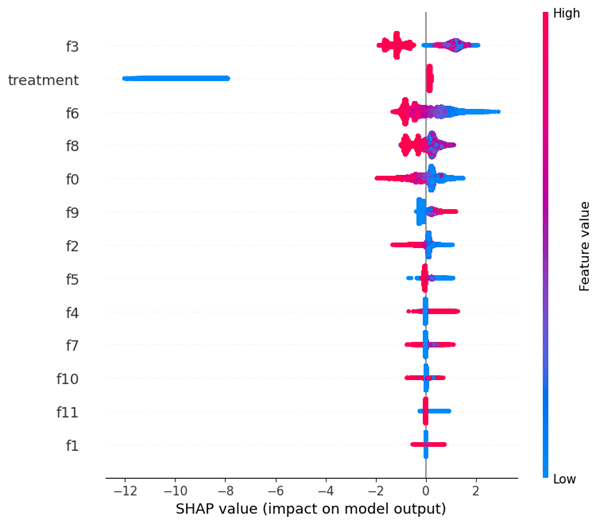
Figure 7 illustrates SHAP summary plot that provides a high-level overview of feature importance by displaying the mean absolute SHAP values for each feature. The length of each bar represents the average impact of a feature on the model’s output, with longer bars indicating greater importance. Feature f3 stands out as the most influential, followed by “treatment” and f6, suggesting their importance to the model relative to other feature values. Conversely, features like f10, f11, and f1 exhibit minimal impact, indicating their limited contribution to the model’s output. This visualization aids in understanding the relative importance of features, guiding feature selection, and revealing underlying data relationships, ultimately enhancing model interpretability and potential refinement. In this figure, no highly correlated pair seem to be apparent, rather the elements of these pairs show up independently, not leading to any conclusions of correlation between specific feature variables.

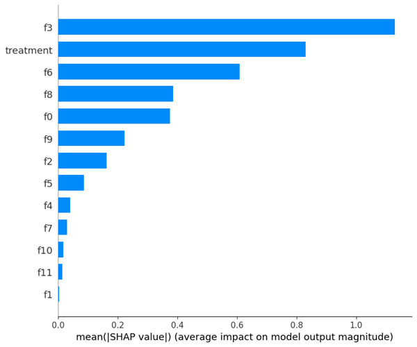
The prominence of certain features in Figures 6 and 7 reveals the true drivers of uplift. The fact that the “treatment” variable ranks highly in importance, despite its negative raw association, confirms that the model is detecting heterogeneity in treatment effects rather than conflating exposure with outcome. This underscores the necessity of a causal framework: traditional models would misinterpret treatment’s correlation, but our uplift approach correctly attributes incremental lift to subpopulations most responsive to marketing. Moreover, the sharp drop in importance after the top three features indicates that much of the predictive signal is concentrated, suggesting opportunities to streamline the feature set for faster training and clearer interpretability without sacrificing performance.

Two Model Approach Results and Discussion

The results of the two-model XGBoost approach, as shown in Table 6, reflect the model’s performance on the treatment group only, as no model is trained on the control group due to the absence of any positive exposure cases. For data values that received the treatment, the model achieves a recall of 0.87, indicating strong performance in identifying those who were exposed. Precision for the exposed class is 0.46, showing that while the model captures most true positives, it also produces a notable number of false positives. The resulting F1 score for the exposed class is 0.60, reflecting a balanced measure of the model’s precision and recall within the treated population, which may be partially due to data imbalance in the treatment group. These metrics demonstrate how the two-model approach focuses solely on estimating treatment effects within the treated group by avoiding the overwhelming presence of negative cases in the control group.

Models (Parameters)	Label (Exposed)	Precision	Recall	F1	Samples
xgboost ‘colsample_bynode’ = 1, ‘eta’ = 0.2, ‘subsample’ = 0.5	0	0.97	0.83	0.89	757716
	1	0.46	0.87	0.60	128293

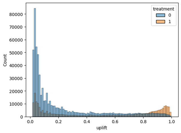
Figure 8 shows the distribution of uplift scores generated by the two-model framework and calculated by subtracting treatment group score by the control group score, trained exclusively on the treated subset and evaluated on the test dataset. The x-axis represents predicted uplift, the estimated increase in probability of exposure due to treatment, and the y-axis represents the number of samples per uplift score. The treated distribution visualizes a range of uplift values containing a noticeable tail of treated high uplift data values, indicating a subset of data values are predicted to have a substantial positive response to treatment. The treated distribution does not resemble a normal distribution, as would be expected from a non-discriminative model, but rather demonstrates the model’s capability of assigning differentiated uplift scores across the population.

To further evaluate model effectiveness, a Qini curve was analyzed, as shown in Figure 9. The Qini curve illustrates the cumulative uplift gained as an increasing portion of the population—ranked by predicted uplift score—is targeted. The steep initial rise of the curve suggests that the model effectively identifies and prioritizes individuals most sensitive to treatment, enabling strategic allocation of marketing resources. The curve then gradually plateaus, indicating diminishing marginal returns as lower-ranked individuals are targeted. The Area Under the Qini Curve (AUC) was calculated to be 0.83, reflecting strong model performance. This high AUC value demonstrates that the model is not only able to distinguish high responders early but also sustains uplift across a the population.

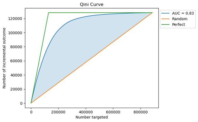
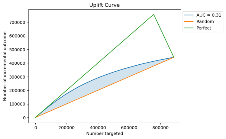
Figure 10 displays the uplift curve for the two-model XGBoost framework, which visualizes the number of incremental outcomes achieved as progressively more individuals are included. The area between the model curve and the random baseline, shaded in blue, yields an Area Under the Uplift Curve (AUUC) of 0.31, indicating effectiveness in identifying users who respond positively to treatment. While not ideal, this AUUC reflects a meaningful gain in targeting efficiency compared to random selection, especially in the early portion of the curve where uplift gains rise rapidly. The divergence between the model and random lines confirms that the model successfully distinguishes high-impact individuals, although the gap from the perfect model suggests room for further refinement or feature enhancement.

To ensure consistent and interpretable evaluation, we report normalized AUUC (nAUUC) or Qini coefficients wherever AUUC is used. nAUUC expresses uplift as a proportion of the maximum possible (ideal) uplift, directly accounting for random and optimal baselines. For example, our nAUUC of 0.834 confirms that the observed uplift represents 83.4% of the theoretical maximum, allowing meaningful comparison across datasets and models irrespective of class imbalance or sample size. This normalization enables reliable, robust claims about model effectiveness and aligns with best practices in uplift modeling literature.

The uplift-specific evaluation confirms that the two-model approach is a strong alternative to the single-model alternative in terms of practical marketing application. Unlike precision or F1 scores, which may be influenced by class imbalance, uplift metrics provide a more realistic estimate of model performance in real-world marketing circumstances. Moreover, the non-uniform distribution of uplift and Qini curve both support the conclusion that the model distinguishes well between susceptible and unsusceptible individuals.

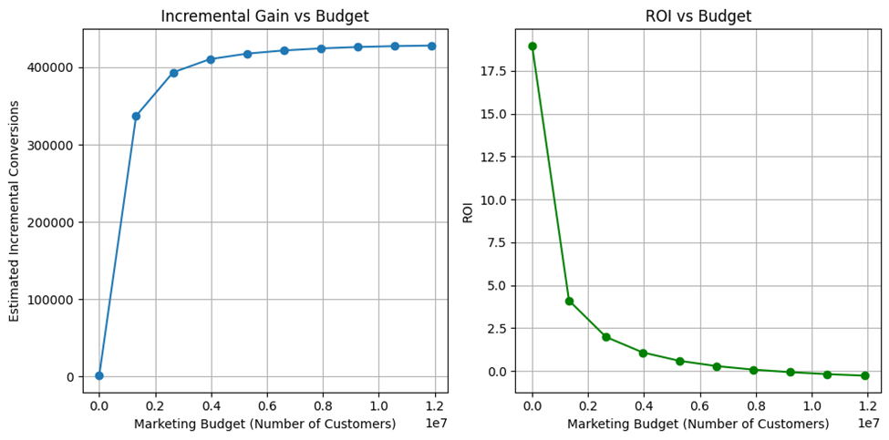
Simulated Financial Practicality

Beyond conventional classification and uplift metrics, we assessed business impact through a simulated budget allocation analysis based off the overall highest performing model, happening to be the undersampled single model approach, specifically with random forest. Customers were ranked by predicted uplift scores, and budget was incrementally allocated from the highest-ranked segments downward. At each level, we measured incremental conversions and ROI, defined as conversions per unit cost. As shown in Figure 11, the Incremental Gain vs. Budget curve indicates that over 80% of incremental conversions can be achieved by targeting only the top ~20% of customers. The ROI vs. Budget curve peaks at low budgets and declines as lower-ranked customers are included, reflecting diminishing marginal returns. These results confirm that the framework not only isolates high-response segments but also provides clear guidance for maximizing ROI through optimal budget allocation. When benchmarked against two-model uplift baselines such as T-learner and X-learner, the two-model approach also performed significantly better. Both baselines performed similar to their single-model counterparts, with negative Qini AUC and uplift AUC values.

Benchmarking and Relative Robustness

To situate our results in the broader uplift modeling landscape, we compare against several published benchmarks. Diemert et al. (2018, 2021) reported uplift AUCs of 0.10–0.15 for tree-based baselines on CRITEO-UPLIFT, while Xu et al. (2022) achieved 0.01514 with their Neural Uplift model on the full dataset. Rzepakowski & Jaroszewicz (2012) demonstrated AUUCs of ~0.25–0.28 on retail datasets using decision-tree methods. Zhao et al. (2019) reported improvements over S- and T-learners in multi-treatment settings, with uplift gains in the 0.20–0.35 range on semi-synthetic Criteo-derived data. More recent neural approaches have reached AUUCs above 0.30 on public benchmarks when incorporating attention mechanisms²⁸. Our two-model XGBoost approach achieved an AUUC of 0.31 and nAUUC of 0.834, placing it in the upper range of reported results while using a framework that remains computationally efficient for large-scale deployment.

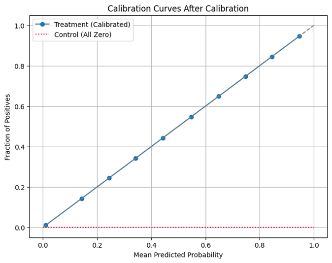
We specifically evaluated calibration of predicted uplift scores to ensure reliability for decision-making. Figures 12 and 13 show pre‑calibration and post‑calibration curves²⁹, with the calibrated model aligning closely to the diagonal, indicating well‑calibrated probability estimates. The Brier score loss for the calibrated treatment model was 0.0242, reflecting high probability accuracy. These scores represent calibrated differences in predicted treatment and control probabilities, making them directly interpretable for targeting decisions in practice. This calibration step ensures the model’s uplift scores are statistically reliable and suitable for real‑world deployment scenarios.

The evaluation also considered how model performance varied across different targeting fractions, ranging from 1% to 50% of the population. Across these fractions, the model consistently achieved higher incremental conversion rates than the random baseline (for example, 1.0000 compared to 0.0331 at 1% targeting). In addition, a sensitivity analysis of the Qini coefficient was carried out for different random seeds and values of max_depth, with results indicating relatively small variations in performance across these settings. By examining both targeting proportions and parameter sensitivities, the analysis provides a broader perspective on model robustness and the conditions under which its uplift predictions remain stable.

Limitations and Future Work

The study has several limitations: the CRITEO-UPLIFT dataset is heavily imbalanced and while we sampled multiple methods of addressing this issue, we ultimately settled on an approach erasing a heavy proportion of this data, which can distort real-world practicality. In addition, causal claimed made in the study rest on unverifiable assumptions, ignoring possible spillovers or delivery failures. The dataset itself has not been deeply analyzed, making room for error.

When it comes to future studies when pertaining to this dataset and uplift marketing in general, future studies may apply new technological advances in the future, especially with advances in neural networks or machine learning models to the problem of uplift marketing. Tighter causal identification and model validation with small online A/B tests would highly increase the quality of the models. In addition to this, future studies may look to unlock the encryption laid upon CRITEO-UPLIFT dataset to increase real world insight upon feature value. With this in mind, more realistic financial simulation would be possible. While financial simulation was conducted in this study, the ultimate practical application of this developed technology, to increase small business marketing efficiency, remains unsatisfied, being a strict limitation on the scope of our work. If completed in conjunction with complementary work in feature annotation or privacy-preserving training would allow for higher deployment performance.

Conclusions

This study explored the effectiveness of uplift modeling in the context of targeted marketing by utilizing the CRITEO-UPLIFT dataset and evaluating various machine learning approaches. The findings highlight the significant importance of addressing data imbalance, with undersampling emerging as the most consistently reliable strategy across different model architectures. This trend was consistent throughout all mediums, with the performance of traditional models such as Random Forest and xgboost notably improved when trained on under sampled data. In addition to this, when paired with appropriate sampling techniques and hyperparameter tuning improvement, despite being incremental, was achieved. Neural networks showed potential but were more sensitive to imbalance and overfitting.

On the other hand, SHAP analysis provided valuable insights into feature contributions, revealing that certain features such as f3, treatment, and f6 were the most influential in predicting exposure—offering practical value for refining marketing strategies given further research into what the feature values represent.

The comparison between single-model and two-model uplift approaches suggested a key trade-off: the two-model strategy improved recall for exposed users, aiding in identifying more potential responders, but at the cost of increased false positives. This finding emphasizes the importance of aligning model choice with business goals—whether that be minimizing cost, maximizing reach, or balancing both and choosing a model which aligns with such a choice.

Ultimately, this research reinforces the practical nature of uplift modeling as a cost-efficient, quantitative marketing tool. By predicting the likeliness of individuals who are most likely to respond positively to marketing exposure, businesses can better allocate resources and streamline marketing campaigns to target potential customers more efficiently. Future work could focus on real-life implementation and results to further advance the field of uplift marketing.

References

1. Statista. Global digital advertising market 2023. Statista. https://www.statista.com/statistics/237974/online-advertising-spending-worldwide/(2024). [↩]
2. P. Gutierrez, J.-Y. Gérardy. Causal inference and uplift modelling: A review of the literature. In Proceedings of Predictive Applications and APIs (PMLR), 67, 1–13 (2017). https://proceedings.mlr.press/v67/gutierrez17a/gutierrez17a.pdf. [↩]
3. N. J. Radcliffe. Using control groups to target on predicted lift: Building and assessing uplift models. Direct Marketing Analytics Journal, 1, 14–21 (2007). [↩]
4. O. Nyberg, T. Kuśmierczyk, A. Klami. Uplift modeling with high class imbalance. In Proceedings of the 13th Asian Conference on Machine Learning (PMLR), 157, 315–330 (2021). https://proceedings.mlr.press/v157/nyberg21a.html. [↩]
5. Y. Zhao, H. Zhang, S. Lyu, R. Jiang, J. Gu, G. Zhang. Multiple instance learning for uplift modeling. arXiv.org, arXiv:2312.09639 (2023). https://arxiv.org/abs/2312.09639. [↩]
6. E. Diemert, J. Thorpe, A. Hankinson, et al. A large scale benchmark for individual treatment effect prediction and uplift modeling. arXiv.org, arXiv:2111.10106 (2021). https://arxiv.org/abs/2111.10106. [↩]
7. M. Belbahri, O. Gandouet, G. Kazma. Adapting neural networks for uplift models. arXiv.org, arXiv:2011.00041 (2020). https://arxiv.org/abs/2011.00041. [↩]
8. H. Wang, X. Ye, Y. Zhou, Z. Zhang, L. Zhang, J. Jiang. Uplift modeling based on graph neural network combined with causal knowledge. arXiv.org, arXiv:2311.08434 (2023). https://arxiv.org/abs/2311.08434. [↩]
9. D. Zhu, D. Wang, Z. Zhang, K. Kuang, Y. Zhang, Y. Kang, J. Zhou. Graph neural network with two uplift estimators for label-scarcity individual uplift modeling. In Proceedings of The Web Conference (WWW), 395–405 (2023). https://doi.org/10.1145/3543507.3583368. [↩]
10. S. R. Künzel, J. S. Sekhon, P. J. Bickel, B. Yu. Metalearners for estimating heterogeneous treatment effects using machine learning. Proceedings of the National Academy of Sciences, 116, 4156–4165 (2019). https://doi.org/10.1073/pnas.1804597116. [↩]
11. X. Nie, S. Wager. Quasi-oracle estimation of heterogeneous treatment effects. Biometrika, 108, 299–319 (2021). https://doi.org/10.1093/biomet/asaa076. [↩]
12. J. Wang, Y. Tan, B. Jiang, B. Wu, W. Liu. Dynamic marketing uplift modeling: A symmetry-preserving framework integrating causal forests with deep reinforcement learning for personalized intervention strategies. Symmetry, 17, 610 (2025). https://doi.org/10.3390/sym17040610. [↩]
13. V. S. Y. Lo. The true lift model: A novel data mining approach to response modeling in database marketing. SIGKDD Explorations Newsletter, 4(2), 78–86 (2002). http://citeseerx.ist.psu.edu/viewdoc/download?doi=10.1.1.99.7064&rep=rep1&type=pdf. [↩]
14. E. Diemert, et al. A large scale benchmark for uplift modeling. HAL Open Science (2018). https://hal.science/hal-02515860. [↩]
15. Rubin, D. B. (1974). Estimating causal effects of treatments in randomized and nonrandomized studies. Journal of Educational Psychology, 66(5), 688–701. https://doi.org/10.1037/h0037350 [↩]
16. L. Breiman. Random forests. Machine Learning, 45, 5–32 (2001). https://doi.org/10.1023/A:1010933404324 [↩]
17. T. Chen, C. Guestrin. XGBoost: A scalable tree boosting system. In Proceedings of the 22nd ACM SIGKDD International Conference on Knowledge Discovery and Data Mining, 785–794 (2016). https://doi.org/10.1145/2939672.2939785. [↩]
18. I. Goodfellow, Y. Bengio, A. Courville. Deep Learning. MIT Press (2016). [↩]
19. F. Pedregosa, G. Varoquaux, A. Gramfort, V. Michel, B. Thirion, O. Grisel, M. Blondel, P. Prettenhofer, R. Weiss, V. Dubourg, J. Vanderplas, A. Passos, D. Cournapeau, M. Brucher, M. Perrot, E. Duchesnay. Scikit-learn: Machine learning in Python. Journal of Machine Learning Research, 12, 2825–2830 (2011). https://jmlr.org/papers/v12/pedregosa11a.html. [↩]
20. R. Kohavi. A study of cross-validation and bootstrap for accuracy estimation and model selection. In Proceedings of the 14th International Joint Conference on Artificial Intelligence (IJCAI), 1137–1143 (1995). https://www.ijcai.org/Proceedings/95-2/Papers/016.pd. [↩]
21. L. Li, K. Jamieson, G. DeSalvo, A. Rostamizadeh, A. Talwalkar. Hyperband: A novel bandit-based approach to hyperparameter optimization. Journal of Machine Learning Research, 18, 1–52 (2018). https://jmlr.org/papers/v18/16-558.html. [↩]
22. P. D. Surry, N. J. Radcliffe. Quality measures for uplift models. Stochastic Solutions white paper (submitted to KDD 2011). http://www.stochasticsolutions.com/pdf/kdd2011late.pdf (2011). [↩]
23. T.-Y. Lin, P. Goyal, R. Girshick, K. He, P. Dollár. Focal loss for dense object detection. In Proceedings of the IEEE International Conference on Computer Vision (ICCV), 2980–2988 (2017). https://doi.org/10.1109/ICCV.2017.324. [↩]
24. N. V. Chawla, K. W. Bowyer, L. O. Hall, W. P. Kegelmeyer. SMOTE: synthetic minority over-sampling technique. Journal of Artificial Intelligence Research, 16, 321–357 (2002). https://doi.org/10.1613/jair.953 [↩]
25. O. Nyberg, A. Klami. Exploring uplift modeling with high class imbalance. Data Mining and Knowledge Discovery, 37, 736–766 (2023). https://doi.org/10.1007/s10618-023-00917-9. [↩]
26. S. M. Lundberg, S.-I. Lee. A unified approach to interpreting model predictions. arXiv.org, arXiv:1705.07874 (2017). https://arxiv.org/abs/1705.07874. [↩]
27. Q. McNemar. Note on the sampling error of the difference between correlated proportions or percentages. Psychometrika, 12, 153–157 (1947). https://doi.org/10.1007/BF02295996. [↩]
28. C. Shen, Z. Du, Y. Liu, Y. Xiong, and W. Chen. Balanced treatment effect estimation in uplift modeling. In Proceedings of the 2023 IEEE International Conference on Data Mining (ICDM), 589–598 (2023). https://doi.org/10.1109/ICDM57529.2023.00071 [↩]
29. A. Niculescu-Mizil, R. Caruana. Predicting good probabilities with supervised learning. In Proceedings of the 22nd International Conference on Machine Learning (ICML), 625–632 (2005). [↩]