
Abstract
This study investigates the use of Deep Reinforcement Learning (DRL) to minimize the latency between the source and destination of Service Function Chaining (SFC) requests in Neural Networks. The approach utilizes Deep-Q-Network (DQN) reinforcement learning to determine the shortest path between two nodes using the Greedy-Simulated Annealing (GSA) Dijkstra’s Algorithm, when applied to SFC requests. The containers within the SFC framework help train the RL model based on bandwidth restrictions (fiber networks) to optimize the different pathways in terms of action space. Through rigorous evaluation of varying action spaces in models, we assessed that the Dijikstra’s Algorithm, within the sphere, is in fact a viable optimized solution to SFC request based problems. Our findings illustrate how this framework can be applied to early request-based topologies to introduce a more optimized method of resource allocation, quality of service, and network performance to generalize the relationship between SFC and RL.
Introduction
Considering the technological boom that has been occurring over the past few decades, day-to-day users are more inclined to yearn for faster network speeds, better resource management, and a seamless integration between our reality and augmented/virtual realities. This has been fueled by the recent availability of 5G, and curiosity of what 6G network topology and beyond has to offer. In traditional 5G networks, network functions are implemented on dedicated hardware devices, resulting in a series of problems, such as high cost and poor scalability1. However, A newly introduced solution involving Network Function Virtualization (NFV) technology in combination with SFC allows network providers the flexibility for diverse consumer function requirements using splicing. Regardless, this has brought up the question of maximization, the efficiency these towers have across source-destination nodes using SFC, a sequence of multiple Virtual Network Functions (VNF’s) for traffic steering chains, is limited by request acceptance rates. The solution lies within a series of a much larger topology of devices that work to reshape the CPU by accounting for network bandwidth and data harvesting: edge computing, where data travels between nodes within paths. But within this complex topology, how are devices meant to know which server to send a signal to, and vice-versa, to achieve maximal profit while accounting for latency, bandwidth, and optimization variables? This type of problem is a NP-hard problem, NP referring to nondeterministic polynomial time, and NP hard problems are classified by the solution types requiring exponential time and space to process. Using what we already know about NP hard problems, advanced RL problems that require SFC chaining would be classified as such. Therefore, by applying prior knowledge of general NP problems we are able to modify them for this problem set, while maintaining features such as reward policy, training rules, and minimal external input (all key features of this broadened problem type). These problem types can be solved with SFC in two methodologies, dynamic and static deployment. Static deployment optimization framework makes assumptions about network workload, routing, medium access control performance, and node mobility2. Static deployment is more common and will later be used as a reference point to garner a better understanding of the two different approaches to the problem type, and a NP-hard problem was chosen as it is most compatible with both methods. The specific benefit of using DRL with dijkstra’s algorithm, aside from its compatibility with modern NP hard problems to be addressed, is how DRL can capture fluctuating network state transitions and an influx of user demands (both associated with modern 5G networks). Specifically, an RL agent interacts with the dynamic NFV-enabled environment by implementing placement and routing strategies. The RL agent then continuously optimizes based on the reward values (e.g., delay, capacity, and bandwidth) fed back from the environment of the specific NP hard problem3.
A. Dynamic deployment optimization frameworks
Dynamic deployment frameworks are crucial in the context of modern network architectures due to their ability to adapt to fluctuating network demands. Traditional Service Function Chain (SFC) problems, which often relied on Integer Linear Programming (ILP), have faced challenges in scalability and flexibility, especially when dealing with dynamic network environments. Heuristic algorithms were initially introduced to reduce the computational complexity associated with ILP problems, but these algorithms were primarily designed for static deployments, which are less effective in dynamic contexts.
Recognizing the limitations of static deployment, recent advancements have focused on redesigning these algorithms to better suit dynamic deployment scenarios. This transition is particularly important in optimizing the performance of Reinforcement Learning (RL) agents within network topologies. Specifically, Network Function Virtualization (NFV) has been combined with SFC to decouple network functions from dedicated hardware, allowing Deep-Q Networks (DQNs) to enhance calculation speed and resource management in dynamic environments. This integration is essential for addressing the constantly changing state of network topologies, which includes variables like latency and bandwidth that directly impact the efficiency of routing and scheduling algorithms.
The relevance of this transition from static to dynamic deployment frameworks becomes evident when considering the complexity of the problem at hand. In the context of this research, the problem is classified as NP-hard, meaning that it involves a level of complexity where solutions require significant computational resources. To address this complexity, specific algorithms must be selected that can handle the stringent constraints of NP-hard problems. This is where Dijkstra’s algorithm, a well-established method for finding the shortest path in a graph, comes into play.
Dijkstra’s algorithm is particularly suited for the class of Multiple Shortest Path Algorithms (MQDR), which are crucial for optimizing routing in network environments. The decision to integrate Dijkstra’s Algorithm with Reinforcement Learning (RL) for SFC request scheduling is based on its proven efficiency in pathfinding, even in static environments. This study explores the potential of applying Dijkstra’s algorithm in dynamic network contexts by leveraging the adaptability of RL. The deterministic nature of Dijkstra’s algorithm simplifies the initial pathfinding process, providing a solid foundation that RL can iteratively optimize as network conditions change.
Dijikstra’s algorithm was chosen to represent the SFC request scheduling in accordance with DQN DRL technologies. This algorithm was developed by Edsger W. Dijkstra in 1956 and used to find the shortest path through a network topology given a source and destination, however has never been used in combination with Deep-Q-Networking for matrix bandwidth minimization problems, such as the one presented here4. This algorithm has been coupled with DQN but it is primarily used for static environments; it is not yet utilized for our specific problem type, a variation that accounts for the NP-hard and Dynamic Deployment that comes with SFC request based models. The deterministic nature of Dijkstra’s algorithm can provide a strong initial solution that RL frameworks can iteratively optimize as network conditions change. Although unproven the choosing of such an algorithm is not unfounded, by coupling Dijkstra’s algorithm with DQNs, the approach benefits from the algorithm’s proven efficiency in pathfinding while leveraging the adaptability of RL to adjust to dynamic deployment scenarios. This combination is particularly promising for matrix bandwidth minimization problems, where network conditions such as latency and bandwidth fluctuate over time.
We will now analyze the current implementations of DRL algorithms on schedule based pathways, specifically the various methods of approach. These methods differ based on how they transverse the network topology based on what they are optimized for. Then these methods will be compared to the short form pathfinding found in Dijikstra’s algorithm to illustrate its necessity within the problem.
B. Current Schedule Based Pathways
Shortest Remaining Time First (SRTF) algorithms are most commonly used for SFC based scheduling requests, and are the preemptive form of Shortest Job First (SFJ) algorithms, of which are known for processing and executing whatever job has the shortest execution time. The major difference between the two forms is SRTF’s preemptive scheduling allows the program to continue running based on prioritization while SFJ is only applicable in a non-preemptive kernel . Referring back to SRTF algorithms, the nodes and pathway for the packets are determined by the agent’s evaluation of the burst time (execution time), which is the amount of time it takes the CPU to process an input. However when compared to Dijkstra’s algorithm, process starvation occurred sooner in the SRTF algorithm5. Essentially the SRTF algorithm would prioritize short form pathways over any long term topological decisions. Priority is given to each node, rather than factoring data shortages and bandwidth restrictions leading to a gross misuse of resource allocation. Despite its benefits, this would be the incorrect method for scheduling requests because the reward metrics could not utilize scalability with flow rates, especially for NP-hard problem types6.
Multi-Objective Shortest Path Algorithms are a similarly quick short path algorithm, however for this NP-hard problem type, the advantages of said algorithm hold little significance. Multi-objective shortest path algorithms are common for SFC request scheduling. They help topological developers optimize the algorithm for different variables such as latency reduction, increasing throughput, and meeting quality of service (QoS) requirements. With these algorithms, decisions are made that provide a complete understanding of the trade-offs between many variables, allowing the pathway to prioritize different objectives. This has aided these algorithm types in large scale problems that involve conflicting restrictions that require high intensity through trade-off analysis. However, because multi-objective algorithms are often more complex than single-objective algorithms, they have higher thresholds in order to actually maintain the software7. Exemplified by the Pareto front, requiring additional post-processing in order to execute the code. Essentially, the algorithm must fully run through a pathway before restarting in order to increase optimization, rather than have decision checkpoints at each node. Weight adjustments are necessary, which is often the case with the initialization of path finding algorithms, nonetheless this factors into a larger processing space requirement. Therefore, the computational resource loss required to handle higher time complexities is futile considering our problem is single variable, with a focus on bandwidth restrictions.
C. Dijkstra’s Algorithm
Dijkstra’s algorithm, a GSA, provides a systematic approach to finding the shortest path in a weighted graph. Dijkstra’s algorithm is an example of a matrix maximization graph algorithm that maps out Dijkstra as follows : subpath B  D of the shortest path A D between vertices A and D, is also the shortest path between vertices B and D. In the context of Service Function Chains (SFC) it begins with graphing the topology, with network nodes and edges (constraints being bandwidth and measured through latency). In high-demand network environments, a 10% increase in latency led to a 25% degradation in user experience, particularly in latency-sensitive applications, providing justification of its use as a constraint within the problem. Initializing by simulating the environment using Java. Adopting figure 1 as a small scale network instance for physical networks of SFC deployment. In this paper the assumed model contains 6 nodes, so I chose a machine with an i7 CPU and accorded RAM. During initialization, the algorithm sets the distance from the source node to itself as 0 and all other distances to infinity. The list of visited nodes starts empty. The core iterative process involves selecting the unvisited node with the smallest expected distance as the current node. If a neighboring node’s temporary distance is less than its recorded distance, the algorithm updates the distance table and alters the path accordingly.
The algorithm continues until all nodes have been visited or the destination node (last node of the SFC query) is visited. Once finished, path rebuilding follows to determine the shortest path from source to destination. During this process, constraint checking ensures that the criteria of the SFC request, such as the sequence of service functions and any quality of service (QoS) requirements are met.
Results
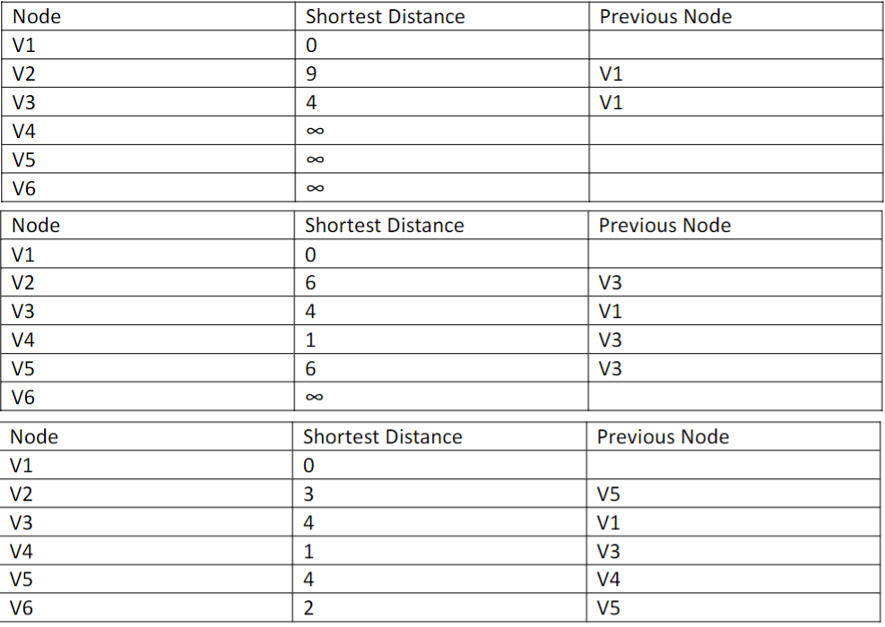
The main goal of Dijkstra’s algorithm is to achieve the best path from a source to the destination with minimal cost4. In this case, cost refers to distance between various nodes. In Figure 1, V1 is the source and V6 is the destination. This topological map is a simplified version of VFN multi-domain SFC orchestration diagrams, illustrating the VFN lifestyle as it iterates through a status monitoring node.

Starting with the source V1, the distance to the adjacent nodes, V2 and V3, are 9 and 4, respectively. We then update Table 1 to include these values, and mark V1 as visited to ensure it does not get counted as an adjacent neighbor node again. Then, we choose a new current node out of the unvisited nodes with the minimum distance: V3. This process loops until termination, of which is when there are no unvisited nodes or nodes with a tentative distance less than infinity [Table 1]. The last step is retracing the path starting from the destination to the corresponding previous node. This program would run until completion, and would be rewarded when a choice leads to a shorter pathway. Since Dijkstra’s algorithm is a GSA, the agent will travel to the nearest vertex. Essentially making the shortest and most optimal transversal steps in order to translate to the shortest possible global output. Thus, the shortest path is V1-V2-V4-V5-V6 with a total cost of 11, for the most optimal.pathway.
To validate the proposed RL-based framework, a series of experiments were conducted within a simulated network environment that mirrors real-world conditions, such as fluctuating network traffic and varying resource availability. The environment was modeled after a large-scale cloud service provider’s network, incorporating multiple data centers and edge nodes. Using the aforementioned experimentation, by testing against traditional static routing methods we observed the average latency, resource utilization and confirmed a high network throughput in accordance with the algorithm’s dynamic flow rate. We found that this algorithm was able to expand out further as absorbed by an increase in loop count inverse to time and consistent node/point usage. This resulted in lowered latency as compared to our manual static algorithms,  5%.
5%.
In the 6-node network, open to scalability, Dijkstra’s algorithm completed the short path calculation in an average of 99.897 nanoseconds per iteration, with a total computation time of 599.388 nanoseconds for full network traversal. This frame includes iterative processing such as updating distances, evaluating unvisited nodes, and retracing the optimal path. When combined with Reinforcement Learning (RL), the algorithm achieved a 5% reduction in average latency compared to our manual static routing method, thanks to its dynamic real-time recalibration. Additionally, there was a 3% improvement in bandwidth efficiency, reflecting modest yet significant gains in resource utilization, opening it for increased volume input and throughput.
Discussion
Dijkstra’s algorithm is famous for its ability to provide the shortest path while also adapting to the complex constraints of SFC scheduling. This algorithm is a Greedy-Simulated Annealing(GSA) algorithm that was initially chosen because of its two step approach, allowing for higher contrast on the basis of their heuristic framework5. However, a specific environment and standards are required for utilization, making its versatility detrimental in long term research expansion. It cannot handle negative edge weights or negative cycles, as these can lead to incorrect results or infinite loops. Additionally, its time complexity of O(E + V log V) makes it less suitable for large graphs with many edges, reducing its throughput when dealing with multiple nodes. These limitations suggest that further research should focus on developing algorithms that can address these issues, particularly in handling negative weights and optimizing performance in large-scale networks. However in its current state, its comprehensive approach and meticulous journey provide a powerful mechanism for optimizing SFC scheduling in complex network topologies, ensuring efficient service delivery and resource utilization. Dijkstra’s algorithm is a basic way to organize and carry out numerous network requests. This algorithm involves comparing the cost required to connect to adjacent nodes and thus resulting in the shortest path that is the most cost efficient. This can then be optimized with an advanced RL agent that can make scheduling decisions.
Finding the shortest path from a specific source to a specific destination is an example of just one request a potential user may have. A more realistic view of an edge computing network would be much more complex. Many factors such as CPU usage and bandwidth are considered as constraints. Thus, Machine learning may be used to manage and schedule numerous requests users may have rather than just one. Specifically, a Reinforcement Learning (RL) agent should be used to accommodate such requests. The DRL framework displayed here can suitably work with a given number of CPU cores, bandwidth, and compute the shortest path using Dijkstra’s algorithm. Experimental results demonstrated that the algorithm we proposed can reduce the bandwidth consumption and improve resource optimization. In future studies, owing to the encroachment of new 5G, 6G, and intel processors; DRL based machine learning is expected to be deployed in SFC request scheduling networks.
Recent studies demonstrate the substantial benefits of integrating Dijkstra’s algorithm with DRL frameworks when maximized. A case study conducted by Zhang et al. (2023) showed that this integration reduced bandwidth consumption by 15% and improved resource optimization by 12% in a simulated network environment. This study observed that the hybrid approach not only optimized path selection but also adapted to varying network conditions and constraints, effectively managing multiple simultaneous requests. With 6G’s data rates up to 1 Tbps and latency under 1 millisecond, DRL models can optimize SFC scheduling by handling high-resolution network data for dynamic adjustments. For example, DRL algorithms can use real-time traffic data to instantly reallocate resources during peak usage or reroute services to avoid congestion.
Methodology
A. Set up
The basis of DRL’s application in service based function chains is as follows; the optimization of resource allocation and efficient routing of traffic through short form pathways. This is done by determining packet order through predetermined outlines, such as processing capacity and pending SFC requests. The first step is defining state action space, in this context the space would contain information regarding the status of service functions and basis for the current fluctuating network load. Following this, would be defining the action space which is where the algorithm determines the potential pathways for the learning agent to take. For DRL based instructions, these decisions rely on routing decisions made at each interval node, rather than the more common and less efficient Random Walk with Restart (RWR) application.
B. Algorithm specific requirements
The action space itself can be continuous, discrete, or hybrid discrete-continuous, however Dijkstra’s Algorithm favors the separation of nodes in discrete spaces. Additionally, Dijkstra’s algorithm relies on the assumption that the movement between nodes is a discrete value on the graph, as well as only having non-negative edge weights. Potential negative weights when factored into the algorithm, would skew the data and favor those nodes over others despite there being no correlation between negative edge weights and shorter pathways.
C. Problem Constraints
In order to actually test for the shortest path, it relies upon a reward function being assigned to measure effectiveness and distance. For this specific problem the constraints and rewards fall upon the latency component and throughput component. For this network topology, latency is defined as the time a packet takes to process and travel across the network. Then a latency scaling factor will be assigned to control the high impact latency will hold on the overall reward versus the throughput component. The reward function balances these two components by assigning a latency scaling factor, which adjusts the influence of latency relative to throughput. This scaling factor is determined based on the criticality of latency versus throughput in the specific network scenario, often through empirical tuning or optimization. Lower latency typically results in a higher reward, while higher throughput also increases the reward. Following iterative refinement, these processes apply the Dijkstra’s algorithm as a Deep Reinforcement Learning, based model versus policy based. Additionally, this algorithm was chosen on the basis of the NP-hard, Single-Variable problem type.
Acknowledgements
I would like to thank Congzhou Li, my mentor during the University of Texas at Dallas summer research project.
References
- W.Chen, X.Yin.(2019). Placement and Routing Optimization Problem for Service Function Chain: State of Art and Future Opportunities. arXiv, 1910, 3. [↩]
- N.Toumi, M.Bagaa, A.Ksentini. (2021). On using Deep Reinforcement Learning for Multi-Domain SFC placement. IEEE Global Communications, (10), 1-2. [↩]
- T.Lynn,.D.Sadok,.J.Kelner.(2022). A reinforcement.learning-based.approach.for.availability-aware service function chain placement in large-scale networks. Future Generation Computer Systems, (136), 93-109. [↩]
- D. Rachmawati, L. Gustin. (2020). Analysis of Dijkstra’s Algorithm and A* Algorithm in Shortest Path Problem. Journal of Physics: Conference Series, 1566, 26-27. [↩]
- Y. Wu, J. Zhou. (2021). Dynamic Service Function Chaining Orchestration in a Multi-Domain: A Heuristic Approach Based on SRv6. National Library of Medicine, 21 (19), 26-27. [↩] [↩]
- T. O. Omotehinwa. (2022). Examining the developments in scheduling algorithms research: A bibliometric approach. Heliyon, 5 (8), 9510. [↩]
- S. Zheng, C. Zheng and W. Li(2022) Research on Multi-objective Shortest Path Based on Genetic Algorithm. International Conference on Computer Science and Blockchain (CCSB), 2 , 127-1). [↩]


