
Jiahua Liang, Sarah Tang, Dr. Susan Fox
Abstract
This work tackles the problem of estimating depth from a single RGB image of a scene. To model the complex relationship between depth and monocular images, we propose a fully convolutional neural network that incorporates skip connections along with encoding and decoding stages to output consistent and detailed depth maps. Additionally, our model is a single convolutional architecture that does not use post-processing strategies; thus, it requires relatively less computational power and time to train when compared to more complex works. Experimental analysis and evaluation with a variety of losses and accuracies show that the end-to-end training process results in a model that performs better than or similar to many past architectures trained on the same dataset. Code and models are publicly available at https://github.com/BitLorax/depth-prediction.
Introduction
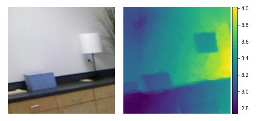
Computer images are two-dimensional by nature. Capturing the third dimension—depth, or the distance between the object and camera—is a monumental task in computer vision. Humans can gauge the depth in an image through experience and common sense, but computers have no prior notion of distance. Thus, many advances have been made to help computers understand depth in the form of a depth map, a matrix of decimal values that represents each pixel’s distance from the camera in meters (Figure 1).
The ability to estimate distance can improve many computer vision applications, such as autopilot systems or assistive technologies. As many self-driving cars see the world through a video feed—Tesla’s cars, for example, use a set of eight surround cameras—depth prediction can improve the accuracy and dependability of their autopilot (Tesla, n.d.). Although such systems also utilize other input forms such as ultrasonic sensors and Lidar, a depth estimation implementation can cross-check with the other predictions, serving as a safety net in the case of errors or anomalies. Robots also benefit from calculating distance; grasping objects is a well-known challenge in robotics, and some basic systems rely on size to determine the object’s distance from the claw. Depth prediction essentially eliminates the need for such computations since it would allow robots to be fully aware of their position in relation to their targets. Other computers, such as those used in robot-assisted surgeries, may also utilize depth. Since precision is crucial in such high-stakes situations, adding depth as another variable can improve the robot’s accuracy and lead to the operation’s success. For example, a predicted depth map may be part of the input to a neural network trained on labeling anatomical features, which can then help it isolate objects or differentiate features that look similar from a certain perspective (Mwiti, 2020).
We propose a deep learning approach to predict depth, utilizing supervised learning to train a model that learns from pre-processed pairs of images and depth maps. Given an RGB image, the algorithm returns depth as a matrix of decimal values that can then be displayed with a colorbar (Figure 1). Our convolutional neural network uses a shrinking-expanding architecture that downsamples and subsequently upsamples the input data, which helps maintain consistency across the entire image. We also concatenated some activations with deeper layers through skip connections to preserve essential structural information. After experimental testing, we evaluate the effectiveness of our methods on the NYU Depth v2 dataset and show that relatively low computational power can still produce excellent results (Silberman et al., 2012).
Background
Supervised Machine Learning
Machine learning is a field of artificial intelligence in which algorithms “learn” to improve their performance on datasets (Ng, n.d.). A “supervised learning” algorithm uses labeled data, where each input comes with an expected output. Thus, it is the machine’s job to generate predictions as close to the expected output as possible.
Standard Neural Networks
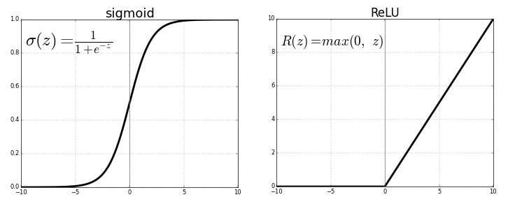
Neural network structures are inspired by biological networks such as the human brain. Their fundamental building block is a node, which, like a neuron, takes and sends information to other nodes. Each node has a set of weights that controls how it processes the input data. To produce an output, it multiplies each weight with its corresponding input and adds a special weight called the bias; then, the node sums up the result and passes it through an activation function, such as sigmoid or ReLU (Figure 2) (Ng, n.d.). These activations help the network generate complexity and learn more advanced features by fitting the data into certain ranges. Without them, neural networks simplify into a polynomial equation, which often fails to capture complicated patterns. After running the sum through the activation function, the result is then sent to other nodes.
Neural networks can be built from hundreds or even thousands of these nodes. All nodes are organized into layers that represent rows of nodes. Each layer takes input from the layer behind it and passes its output to the layer in front of it. This structure is represented in Figure 3.
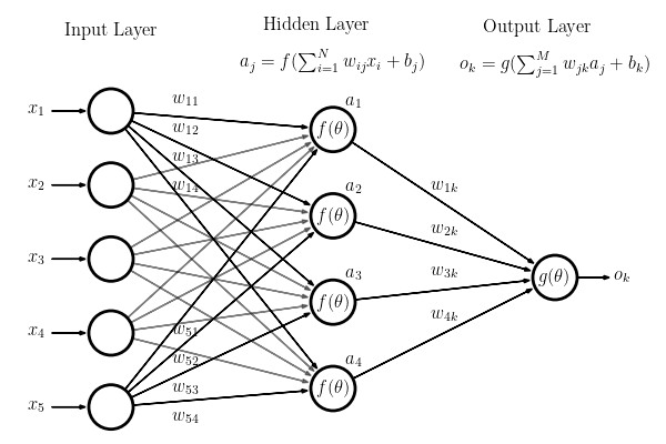
In the most common type of neural network, known as a fully connected neural network, each node takes in the outputs of all nodes in the previous layer. The node then sends outputs to all nodes in the following layer. Each of these outgoing connections has a set of specific weights that are applied to the node’s inputs; in other words, the output that node i sends to node j is different from the output sent to node k.
These values are commonly represented in matrices as matrix calculations are optimized on modern GPUs. When computing the output of each node, we thus find the output matrix that holds values for each node in the following layer, which can be calculated by the equations
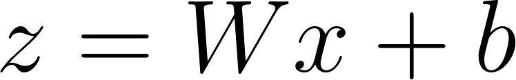
where z contains the weighted sums, x is the input, W and b are the weights and biases, f is the activation function, and a contains the activation values.
The first layer in a neural network is the input to the network; thus, the number of nodes in this layer is the number of input values. Similarly, the final layer of the neural network is the prediction of this network and has a number of nodes corresponding to the number of expected predictions. The layers in the middle are commonly known as hidden layers since we cannot directly control their computations—they work like a black box that transforms the input into predictions (Ng, n.d.). In order to improve its accuracy, the neural network updates its weights. First, the model generates the output in a process called forward propagation and compares it with the ground truth using a loss function, such as mean squared error or categorical cross-entropy. Mean squared error (3), for example, finds the squared difference between truth and predictions.
The goal of the model is to minimize this loss in a process called backpropagation. The network calculates the derivatives of the loss function with respect to each parameter, starting with the final layer and then using the chain rule to calculate derivatives for each previous layer. These derivatives “point” toward the local minima as a positive slope suggests minima is “behind” the current point, while a negative slope indicates that the minima is “in front” of the current point. Thus, for each weight, the model subtracts the derivative multiplied by a constant—denoted as alpha—called the learning rate (4), moving it closer to minimum loss (Ng, n.d.).
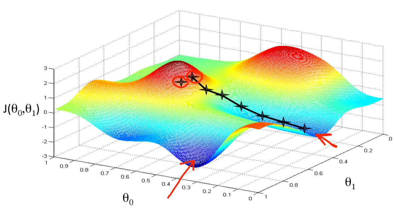
To visualize this idea, commonly known as gradient descent, the learning problem can be represented as rolling a ball down a hill (Figure 4). The hill is the loss function calculated over all parameter values, and the ball is our current model. Gradient descent moves the position of the model in the direction that minimizes loss; thus, with our analogy, the ball rolls down the steepest part of the hill, eventually finding the local minima and finishing its descent.
Forward propagation and backpropagation are repeated over many batches of data. Each batch is a fraction of the entire dataset that the model looks over before updating its parameters. Batches are then grouped into epochs, where one epoch is one iteration over the entire dataset. After tens or hundreds of epochs, the model’s loss will begin to flatten out, which suggests that it is done training (Ng, n.d.).
Convolutional Neural Networks
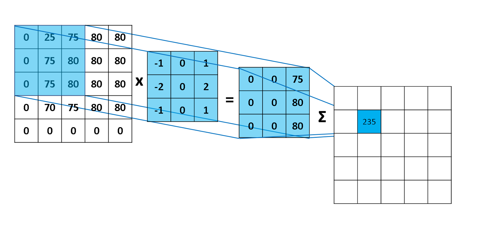
Unlike fully connected neural networks, convolutional neural networks (CNN) do not connect each node with every node in its previous and following layers. Instead, nodes are organized into 2-D matrices, and layers consist of n matrices stacked together. The weights of a layer are also organized into an n-stack of smaller 2-D matrices. Each weight stack, known as a filter, applies its i-th 2-D matrix to the i-th 2-D input matrix in the convolution process: the weight matrix scans over the input values, multiplying each weight with its overlapping value and finding the sum of the products; this sum then goes through an activation function into one cell in a new 2-D matrix (Ng, n.d.).
Figure 5 illustrates an instance in the convolution process. The first matrix is the input, the second matrix is the filter, and the overlapping values in blue are multiplied and then summed. Note that the figure does not show the sum going through an activation function. Each filter forms a complete matrix, and these matrices are stacked together as the input for the following layer.
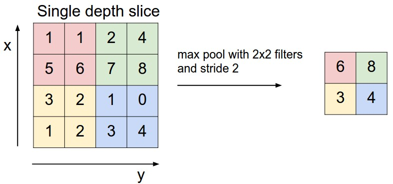
One problem with normal convolutions is that the matrix dimensions will almost always shrink after going through a filter. In order to counter this side-effect, we add padding to the sizes of each input matrix. If a convolution shrinks a matrix from 5-by-5 to 3-by-3, for example, we can pad the 5-by-5 with 1 layer of zeros; thus, the convolution shrinks the padded 7-by-7 matrix into a 5-by-5, thereby maintaining the original resolution. A padded convolutional layer also gains greater exposure to edge and corner values, which helps the model learn potentially valuable information from the input. Padding that keeps the resolution constant is called same padding. CNNs also commonly use pooling layers along with convolutional layers. The pooling layer has a similar type of filter, but instead of applying weights, the layer performs a function on all values in the filter. Max pooling, for example, passes the maximum value in the filter onto the next matrix (Figure 6). This is commonly used to lower dimensions of the matrices as values in each filter are compressed into a single number, which helps with bringing learned features together and allowing the model to process a more global representation of the data. Pooling also helps with cleaning up noise and unwanted artifacts since it essentially simplifies the input data.
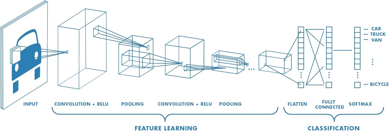
Basic CNNs have multiple convolutional and pooling layers to slowly decrease the dimensions of their matrices. Once the number of values shrinks to a manageable size, the network flattens its stack of matrices into a single row, similar to that found in standard neural networks. These rows then pass through fully connected layers and eventually return a row of output nodes. A complete diagram of this process is shown in Figure 7.
Related Works
Depth prediction is an extremely popular field in deep learning as hand-crafted features cannot capture complexity as well as learned weights. Thus, there have been numerous approaches to this problem.
Fully Convolutional Neural Network
Laina et al., 2016, trained an end-to-end CNN model for predicting depth from a single RGB image. Their network replaces the dense layers found at the end of a basic CNN with up-projection blocks that upscale the output using residual blocks along with reverse pooling and convolutions. The model optimizes with the reserve Huber loss that balances the impact of high and small residuals. After training, it surpasses many famous architectures with less data and fewer parameters. This compression and expansion architecture is incorporated as our model’s encoding and decoding stages, which allows it to learn global features while also outputting a high-resolution image.
Unsupervised Learning
As opposed to supervised learning, unsupervised learning trains models without using ground truth depth data. These methods are an alternative approach to depth prediction that we do not ultimately pursue.
Godard et al., 2017, used a depth map as an intermediate step in reconstructing one image with another; given left and right RGB images from a binocular camera, the function learns the depth required to rebuild the image from the other. Thus, this method does not use ground-truth depth maps, allowing it to use a wider range of data that is not as hard to collect. Similarly, Zhou et al., 2017, built a model that learns depth as an intermediate to pose translation. Given a view of a scene and a new relative pose, the network is trained to synthesize a new image of the scene with the new position and orientation. In doing so, the model must learn a depth map as depth is crucial to generating images with different poses.
Image Segmentation
While image segmentation—the classification of individual pixels—itself is a broader problem than depth prediction, the two tasks are similar in that outputs are in the form of images instead of values or classes. Thus, models used for segmentation problems are strongly related to depth prediction.Ronneberger et al., 2015, designed a fully convolutional neural network called U-Net that uses convolutions and max pooling layers to reduce the size of the input. Whereas most CNNs now move on to fully connected layers, the U-Net begins to upsample the resolution in order to produce an image. This process uses upsampling layers and convolutions while also concatenating activations from previous layers to the upsampling layers; these connections allow the model to better learn structure as the initial convolutions destroy the structure of the input image. We also employed these concatenations between layers in our own architecture as depth prediction heavily relies on remembering the input image’s structure.
Conditional Random Fields
Liu et al., 2015, used a CNN that feeds into a conditional random field (CRF) to predict depth maps from a single image. Their algorithm begins by splitting the input image into “superpixels,” which are small homogeneous pixel regions. They then feed the input image into a CNN with sequences of convolutions and pooling layers, ending with a series of fully connected layers that output depth values for each superpixel. The CRF then goes over each node and its neighbors, feeding their values into predefined functions that learn to minimize a set error; the functions in this specific CRF are designed to refine the overall quality of the produced depth map, for example by smoothing gradients or removing noise. While the CRF part of the network is not integrated into our model, this work’s fully connected layers partly inspire the idea of a bottleneck that learns global features; however, we use convolutions instead of fully connected layers in our approach.
Data Preprocessing and Generation
Data Augmentation
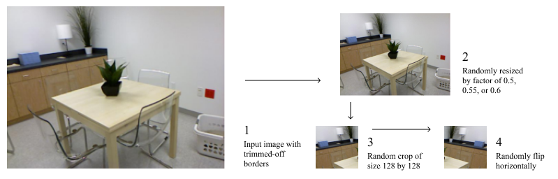
Since labeled depth datasets are usually relatively small, we must expand the number of images we can feed into the neural network in a process called data augmentation. The NYU Depth v2 dataset (Silberman et al., 2012) provides images of resolution 640 by 480 pixels, but our model takes inputs of size 128 by 128 pixels. To reduce the resolution, we first cropped out the white border and randomly downsize the image by a factor of 0.5, 0.55, or 0.6; then, we take a random 128-by-128 crop from the downsized image. Although certain crops may share parts of the image, our random cropping method can produce tens of semi-unique images from a single downsized picture. Next, we randomly flipped the cropped image horizontally as it creates another valid example; however, we did not flip it vertically as it does not make sense to have upside-down objects. This process is visualized in Figure 8.
Data Generation
Augmenting data can create huge datasets, so it is not feasible to load all of the data into RAM for training. Thus, we built a custom data generator in Tensorflow to fetch images from their stored files when they are needed and randomly augment them right before they are fed into the network. In doing so, we negate the need to store all variations in the hard disk and RAM; the generator simply uploads and augments the images in parallel with training.
Model Architecture
Overview
Whereas standard CNNs output classes or regression values, our model must output an image. Thus, we cannot use the standard CNN architecture of shrinking matrix sizes and fully connected layers; instead, our model upsamples the matrices after shrinking them (Figure 9). Like U-Net (Ronneberger et al., 2015), we have two stages: an encoding stage and a decoding stage. The former compresses matrix sizes, allowing the model to learn global attributes of the image. The latter then increases the matrix resolution, effectively “decoding” the encoding stage’s result to produce a depth map.
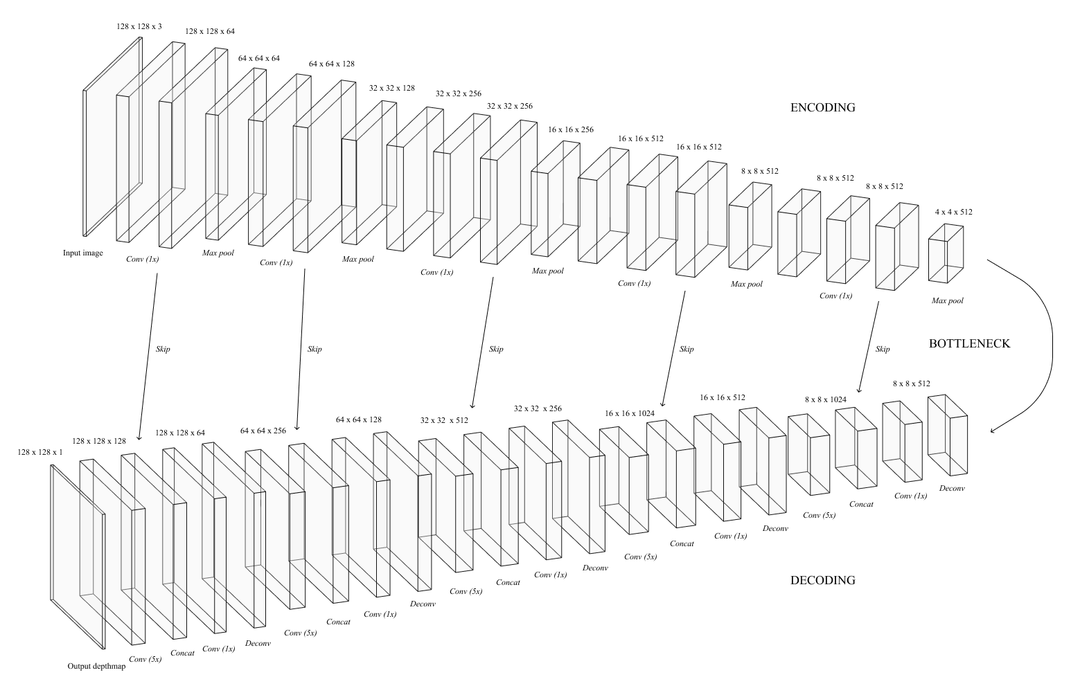
Encoding Stage
For the encoding stage, we used the VGG-16 architecture (Simonyan et al., 2015), a famous network that has yielded strong performance in other works. It consists of 5 blocks of convolutional and pooling layers, with each block reducing the image resolution by half. Each convolution uses a 3 by 3 kernel with same padding so that the resolution stays constant with each convolutional layer. The outputs from convolutions that are right before pooling layers are saved for later; during the decoding process, they “skip” over the mid-section of the network and concatenate with a layer in the decoding stage. At the end of each block is a pooling layer, which uses a 2-by-2 filter with a stride of 2 that cuts the resolution in half. Since VGG-16 is used for classification, it has fully connected layers and a softmax attached to the end. However, fully connected layers completely disrupt spatial information as the matrices are essentially flattened into rows; thus, it is usually detrimental to networks that produce images. For our model, we cut off everything after the final max pooling layer and attach the decoding stage to the end instead.
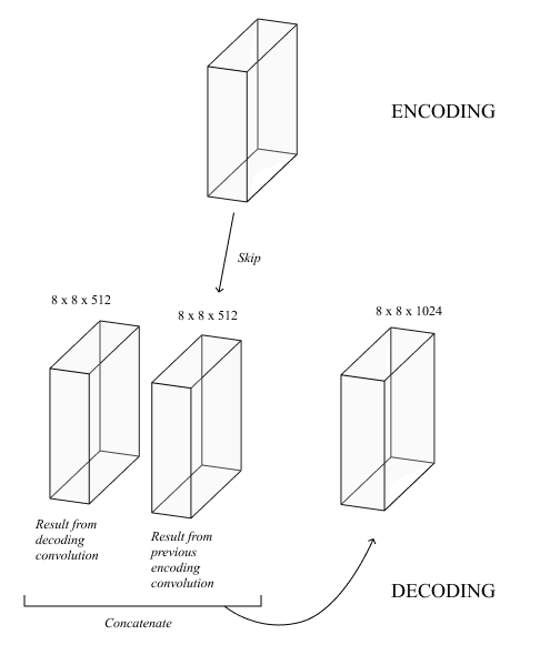
Decoding Stage
The decoding stage takes the encoding stage’s output and converts it into a depth map. This stage contains 5 blocks of deconvolution and concatenation layers. Each deconvolution layer increases the resolution by a factor of two, thereby reversing the effect of the previous stage’s pooling layers. Each deconvolution is then followed by a skip connection, where the deconvolution result is concatenated with its corresponding layer from the encoding stage (Figure 10). This technique helps the model maintain the structure of the overall image as much of this information is lost during the encoding process. Finally, we capped off the decoding stage with a convolutional layer that compresses the 128 separate matrices into a depth map, which is a single 128 by 128 matrix.
Experimental Analysis
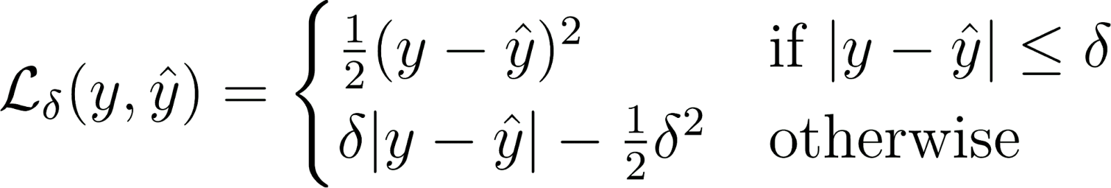
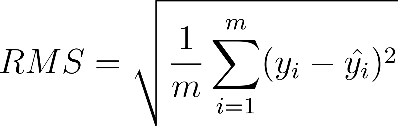
After creating a base architecture, we began to improve its learning speed and results by experimenting with different hyperparameters, or user-defined attributes of the model such as the number of layers and the learning rate. Through our trials, we trained on the Huber loss function (5) with delta = 1. This loss is robust to outliers while also having small gradients with lower residuals, which allows it to better converge toward the local minima of the cost function. However, due to its complexity, we also use root mean square (RMS) error (6), a simple and common regression metric that punishes large errors, to interpret the success of our experiments.
To start, we tested different learning rates, which determines how much the weights shift in each backpropagation step. This hyperparameter is important since small learning rates lead to slow convergence while high learning rates fail to converge. We kept all other factors constant, and after testing the range from 0.001 to 0.1 for 10 epochs, we settled on an initial learning rate of 0.005.
Next, we evaluated the Adam, Nadam, Stochastic Gradient Descent (SGD), and RMSprop optimizers, which all serve the purpose of updating a model’s weights given the derivatives of the error. SGD updates weights with gradient descent for each training example. RMSprop introduces an automatically decreasing learning rate based on the magnitude of past gradients, which often leads to a more steady convergence. SGD and RMSprop can also use momentum—calculated with an exponentially weighted average of past gradients—in each gradient step, which helps the model avoid local minima and converge faster. Adam, one of the most popular optimizers, combines ideas from RMSprop and SGD with momentum to both update the learning rate and also calculate momentum; Nadam is simply a variant of Adam that uses a different momentum calculation known as Nesterov momentum. For each optimizer, we train a base model at a constant learning rate of 0.005. We found that Adam and SGD with momentum are the two best optimizers for our task (Table 1), but after evaluating them on longer epochs and a decaying learning rate, we chose SGD with momentum for our model due to its higher overall performance.
| Optimizer | RMS | Huber |
| Adam | 1.5004 | 0.7434 |
| Nadam | 1.5068 | 0.7264 |
| SGD (Beta = 0) | 1.9073 | 0.9763 |
| SGD (Beta = 0.9) | 1.4351 | 0.6951 |
| RMSprop (Beta = 0) | 1.5383 | 0.7576 |
| RMSprop (Beta = 0.9) | 1.5416 | 0.7502 |
Since SGD does not change the learning rate by itself, we also analyzed exponential and adaptive learning rate decay. We eventually chose adaptive decay since it is more versatile and complex as opposed to a steadily decreasing learning rate. Our experiments suggest that an adaptive decay with a patience of 5 epochs, 0.005 initial rate, 0.0001 minimum rate, and a factor of 0.3 results in optimal performance with a relatively quick convergence time.
With training parameters finalized, we began evaluating the effects of architectural changes to the model. Starting with adding convolutional layers before every skip connection in the encoding stage, we found that the RMS error worsened. This performance suggests that VGG-16 (Simonyan et al., 2015) alone is enough to capture all of the information we need for encoding and that adding more convolutional layers to the start of the model is redundant. Next, we added convolutions to the bottleneck between the encoding and decoding stages. After testing some configurations, we find that adding two convolutions with same padding and filters of size 1 is optimal; we choose 1-by-1 filters instead of 3-by-3 since the matrix size in the bottleneck is relatively small compared to other layers.
Our original decoding stage starts out as a series of deconvolutions that upsamples the resolution by a factor of 2. Thus, to output a depth map of equal resolution to the input image, we stacked 5 of these deconvolutional layers together. However, this approach lacks complexity. We quickly hit a problem with underfitting as there are simply not enough layers to “decode” the output of the bottleneck; thus, the model struggles to improve, even when presented with huge amounts of data.
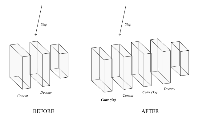
We solved this problem by adding convolutions that kept all 3 dimensions of the input constant. After adding 1 convolutional layer before each skip connection and 5 convolutional layers after each skip connection (Figure 11), adding more complexity did not improve the error (Table 2); thus, this is our optimal setup for the decoding stage. However, adding on the 1-by-1 convolutions in the bottleneck does not have any effect. The extra convolutions in the decoding stage likely nullify the benefit of extra processing in the bottleneck, so we can exclude the bottleneck convolutional layers.
| Architecture | RMS | Huber |
| 1 conv before, 3 conv after | 1.1551 | 0.4863 |
| 1 conv before, 4 conv after | 1.1196 | 0.4624 |
| 1 conv before, 5 conv after | 1.0959 | 0.4505 |
| 2 conv before, 2 conv after | 1.1428 | 0.4912 |
| 2 conv before, 3 conv after | 1.1629 | 0.4961 |
| 2 conv before, 4 conv after | 1.1219 | 0.4686 |
| 2 conv before, 5 conv after | 1.1652 | 0.4999 |
Final Results
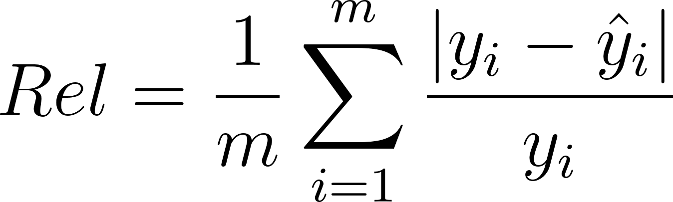
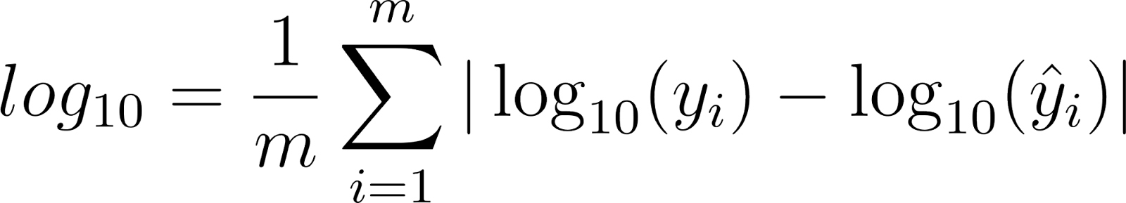
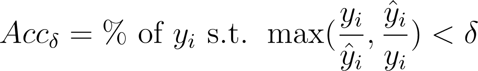
After securing a few more details, we trained our model for 100 epochs using SGD with momentum and adaptive learning rate decay. Our model achieved a test Huber loss of 0.2793 and a 0.8173 RMS error, a significant improvement from our initial results. To compare with past works, we also calculated the final absolute relative error (7), log10 error (8), and accuracies at 3 thresholds (9), which are common evaluation metrics for this problem (Eigen et al., 2014; Karsch et al., 2012).
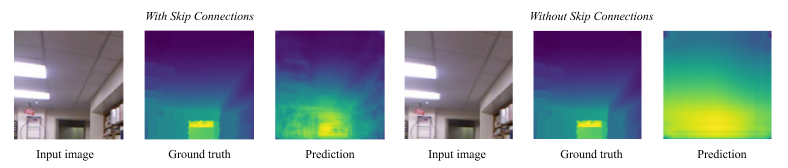
As shown in Table 3, our model’s performance exceeded or matched many past works that are also evaluated on the NYU Depth v2 dataset (Silberman et al., 2012) even though it uses fewer computational resources and a shorter training time. One potential reason for our result is the use of skip connections. While many strategies can help the model learn complexity without sacrificing the image structure, skips prove to be simple and effective. As shown in Figure 12, our finalized model outputs a smooth gradient when we remove these connections. Thus, architectures without skips may need more convolutions or alternative strategies to achieve similar performance.
| Paper | RMS | Rel | log10 | Acc Delta = 1.251 | Acc Delta = 1.252 | Acc Delta = 1.253 |
| Karsch et al. (2012) | 1.12 | 0.374 | 0.134 | – | – | – |
| Ladicky et al. (2014) | – | – | – | 0.542 | 0.829 | 0.941 |
| Liu et al. (2014) | 1.06 | 0.335 | 0.127 | – | – | – |
| Eigen et al. (2014) | 0.907 | 0.215 | – | 0.611 | 0.887 | 0.971 |
| Ours | 0.8173 | 0.2458 | 0.0968 | 0.6018 | 0.8833 | 0.9672 |
However, our model still falls short of some other deep learning approaches that employ similar convolutional neural networks with other strategies, such as residual blocks or conditional random fields. For example, Laina et al., 2016, used a deep residual architecture and unique up-projection layers that can capture more specific features in the dataset, thereby improving their test metrics. We lacked the computing power to process a larger dataset or further expand our design with other techniques that can be beneficial to this regression-based problem. Improving in these areas can help our model develop a more complex understanding of depth data.
Future Work
A U-shaped architecture along with skip connections proves to be very effective, but there are many other ideas that can be implemented in the future.
Residual blocks (Laina et al., 2016) can be a great addition to our network due to their versatility. Our model’s architecture is based on experimental results comparing the effects of adding or removing layers. However, setting the model’s architecture in stone may not be optimal for its performance. Thus, with residual blocks, we let the machine decide its own network depth. Shortcuts allow us to build extremely deep networks without running into the problem of gradient explosion as the model can essentially cut off useless layers. This strategy not only improves performance but also saves time as it lessens the need for detailed architectural experimentation.
Another potential improvement is incorporating a conditional random field (Tsang et al., 2019) into the end of the model. This serves to refine the input and produce a smoother and more accurate image. We can train it along with the rest of the model so that it works as a special layer that teaches the model to create a more visually accurate depth map.
Lastly, integrating this model into an unsupervised learning setting can allow us to train a more complex architecture due to having a vastly greater amount of data. Since depth maps are time-consuming and expensive to create, having an unsupervised learning algorithm find depth all on its own frees us from only using depth datasets. Zhou et al., 2017, for example, used depth as an intermediate in a pose generation model. As depth is crucial to generating this problem’s output, they are able to train a depth predictor without explicit depth data. It is possible to use our current model as part of a similar network.
Conclusion
In this work, we present a solution to depth prediction from a single RGB image. Our method employs an end-to-end approach, using a fully convolutional neural network with multiple skip connections and a U-shaped encoding-decoding architecture. The model borrows from VGG-16 (Simonyan et al., 2015) for its encoding stage and uses connections between the two stages that are heavily inspired by the U-Net (Ronneberger et al., 2015). These skip connections prove to be integral to the architecture by preserving the original image structure, which helps the model more easily build an accurate depth map. In addition to receiving the skip connection activations, our unique decoding stage upsamples the image into its original resolution while applying multiple convolutions to add complexity; trial runs show that this stage is the most complex and important part of our model, significantly contributing to the output. After training on the NYU Depth v2 dataset (Silberman et al., 2012), our final architecture learns to output accurate depth maps and surpasses or performs on par with many past models (Table 3) while requiring fewer computational resources and less time. In the future, we can improve our model with other deep learning strategies, including residual nets, conditional random fields, and unsupervised learning.
References
AstroML Neural Network Diagram. (n.d.). Retrieved June 9, 2020, from https://www.astroml.org/book_figures/chapter9/fig_neural_network.html
Divam. (2019, June 6). A Beginner’s guide to Deep Learning based Semantic Segmentation using Keras. Retrieved from https://divamgupta.com/image-segmentation/2019/06/06/deep-learning-semantic-segmentation-keras.html
Eigen, D., Puhrsch, C., & Fergus, R. (2014). Depth Map Prediction from a Single Image using a Multi-Scale Deep Network. NIPS’14: Proceedings of the 27th International Conference on Neural Information Processing Systems, 2, 2366-2374. doi:10.5555/2969033.2969091
Godard, C., Mac Aodha, O., & Brostow, G. J. (2017). Unsupervised Monocular Depth Estimation with Left-Right Consistency. The IEEE Conference on Computer Vision and Pattern Recognition (CVPR), 270–279. doi: 1609.03677
Image segmentation. (n.d.). Retrieved May 27, 2020, from https://www.tensorflow.org/tutorials/images/segmentation
Karsch, K., Liu, C., & Kang, S. B. (2012). Depth Extraction from Video Using Non-parametric Sampling. Computer Vision – ECCV 2012 Lecture Notes in Computer Science, 775-788. doi:10.1007/978-3-642-33715-4_56
Ladicky, L., Shi, J., & Pollefeys, M. (2014). Pulling Things out of Perspective. 2014 IEEE Conference on Computer Vision and Pattern Recognition. doi:10.1109/cvpr.2014.19
Laina, I., Rupprecht, C., Belagiannis, V., Tombari, F., & Navab, N. (2016). Deeper Depth Prediction with Fully Convolutional Residual Networks. 2016 Fourth International Conference on 3D Vision (3DV). doi: 10.1109/3dv.2016.32
Le, J. (2019, October 23). How to do Semantic Segmentation using Deep learning. Retrieved from https://nanonets.com/blog/how-to-do-semantic-segmentation-using-deep-learning/
Li, F.-F., Krishna, R., & Xu, D. (n.d.). Convolutional Neural Networks. Retrieved June 13, 2020, from https://cs231n.github.io/convolutional-networks/
Liu, F., Shen, C., & Lin, G. (2015). Deep convolutional neural fields for depth estimation from a single image. 2015 IEEE Conference on Computer Vision and Pattern Recognition (CVPR). doi: 10.1109/cvpr.2015.7299152
Liu, M., Salzmann, M., & He, X. (2014). Discrete-Continuous Depth Estimation from a Single Image. 2014 IEEE Conference on Computer Vision and Pattern Recognition. doi:10.1109/cvpr.2014.97
Mwiti, D. (2020, February 11). Research Guide for Depth Estimation with Deep Learning. Retrieved June 1, 2020, from https://heartbeat.fritz.ai/research-guide-for-depth-estimation-with-deep-learning-1a02a439b834
Ng, A. (n.d.). Coursera Deep Learning. Retrieved June 5, 2020, from https://www.coursera.org/learn/neural-networks-deep-learning/home/welcome
Prabhu, R. (2019, November 21). Understanding of Convolutional Neural Network. Retrieved June 13, 2020, from https://medium.com/@RaghavPrabhu/understanding-of-convolutional-neural-network-cnn-deep-learning-99760835f148
Robinson, R. (2017, April 7). Convolutional Neural Networks Basics. Retrieved June 13, 2020, from https://mlnotebook.github.io/post/CNN1/
Ronneberger, O., Fischer, P., & Brox, T. (2015). U-Net: Convolutional Networks for Biomedical Image Segmentation. Lecture Notes in Computer Science Medical Image Computing and Computer-Assisted Intervention – MICCAI 2015, 234–241. doi: 10.1007/978-3-319-24574-4_28
S., S. (2020, June 16). Gradient Descent: All You Need to Know. Retrieved June 11, 2020, from https://hackernoon.com/gradient-descent-aynk-7cbe95a778da
Sharma, S. (2019, February 14). Activation Functions in Neural Networks. Retrieved July 1, 2020, from https://towardsdatascience.com/activation-functions-neural-networks-1cbd9f8d91d6
Silberman, N., Hoiem, D., Kohli, P., & Fergus, R. (2012). Indoor Segmentation and Support Inference from RGBD Images. Computer Vision – ECCV 2012 Lecture Notes in Computer Science, 746–760. doi: 10.1007/978-3-642-33715-4_54
Simonyan, K., & Zisserman, A. (2015). Very Deep Convolutional Networks for Large-Scale Image Recognition. ICLR. doi: 1409.1556
Team, K. (n.d.). Keras. Retrieved June 4, 2020, from https://keras.io/
Tesla. (n.d.). Autopilot AI. Retrieved July 1, 2020, from https://www.tesla.com/autopilotAI
Tsang, S.-H. (2019, March 20). Review: CRF-RNN-Conditional Random Fields as Recurrent Neural Networks (Semantic Segmentation). Retrieved June 13, 2020, from https://towardsdatascience.com/review-crf-rnn-conditional-random-fields-as-recurrent-neural-networks-semantic-segmentation-a11eb6e40c8c
Zhou, T., Brown, M., Snavely, N., & Lowe, D. (2017). Unsupervised Learning of Depth and Ego-Motion from Video. The IEEE Conference on Computer Vision and Pattern Recognition (CVPR), 1851–1858. doi: 1704.07813


