NHSJS Reports

Classical Shadows For Entanglement Witness Estimation

September 1, 2026

Abstract

The numerical data obtained for the Bell witness indicates that the estimation cost is more influenced by witness support than the size of the entire system. Witnesses of entanglement prove that entanglement is present without carrying out a complete tomography, in a straightforward scientific manner. The calculations carried out here can be considered as case studies. The application of these methods for larger systems implies the knowledge about the constraints which define the costs of witness estimation. Four experiments are carried out in order to study this question. The first one aims at investigating how the estimation error is dependent on the number of measurements carried out. For both local Pauli and global Clifford measurements, the error decreases as the number of measurements grows, at close to an inverse-square-root rate. The second experiment consists of the noise of depolarizing type. This model’s shadow estimation follows the witness value from $Tr\left( W\rho(p) \right) = - \frac{1}{2} + \frac{3}{4}p$ , and ensures the proper consistency with the expected threshold from $p = \frac{2}{3}$ . The third application brings the two-qubit witness to bigger systems. In the process of growing the system to n=6, the precise witness value holds steadily. For our example, the empirical variance and the calculated number of shots remain mostly unchanged. Our fourth experiment is based on the modification of the Bell witness using both the local and the more remote Pauli perturbations. In particular, we used the zero mean perturbations whereby the observables overlap significantly.

Introduction

Quantum information theory studies how information is processed in quantum systems¹. The basic unit of a quantum system is a qubit, and it can be written in the form

$\left| \psi \right\rangle = \alpha\left| 0 \right\rangle + \beta\left| 1 \right\rangle,\quad\quad|\alpha|^{2} + |\beta|^{2} = 1.$

An n-qubit system exists in the Hilbert space $(\mathbb{C}^{2})^{\otimes n}$ , which demonstrates that the dimensions of the state space increase exponentially with the number of qubits present. The measurement in quantum physics is probabilistic in nature. Let’s say that the system has a density operator $\rho$ and measure an observable represented by a projector $\Pi_{m}$ . The probability of obtaining outcome m is given by this expression

$p(m) = Tr\left( \Pi_{m}\rho \right).$

What one measurement can tell us is very limited about the quantum state. For this reason, it is necessary to perform many measurements, which is another reason why full quantum state tomography is such a computationally expensive process.².

One of the most important features of quantum systems is entanglement. A bipartite state is separable if it has the form

$\rho_{AB} = \sum_{k}p_{k}\,\rho_{A}^{(k)} \otimes \rho_{B}^{(k)},\quad\quad p_{k} \geq 0,\ \sum_{k}p_{k} = 1.$

States that cannot be written this way are entangled. Entanglement is an important resource across quantum information, from quantum algorithms to quantum communication and quantum sensing³^,⁴^,⁵.

One way to detect entanglement is with an entanglement witness⁶^,⁷^,⁸. A witness is an observable $W$ such that

$Tr(W\sigma) \geq 0\quad\text{for every separable state }\sigma,$

but

$Tr\left( W\rho_{target} \right) < 0$

for the target entangled state. So if the witness expectation value is negative, the state must be entangled. However, witnesses can still be hard to measure if they act on many qubits.

Classical shadows estimate observables directly from randomized measurements without reconstructing the full density matrix⁹. Related randomized measurement and shadow tomography frameworks are developed in Refs¹⁰^,¹¹. They are a good tool for witness estimation. The main question in this paper is: when a witness is estimated using classical shadows, what controls the cost? This study uses cost as a synonym for the needed amount of measurement shots to accomplish a trustworthy estimate.

The classical shadow approach and randomized measurements have since evolved in several ways relevant to this study. One of the lines looks into how the ensemble of measurements influences the estimation cost in terms of noisy shadow complexity¹²^, Pauli-invariant ensembles¹³^, locally entangled measurements that change the scaling with Pauli weight¹⁴^, and common randomized measurements for improved property estimation¹⁵. A second line targets robustness and error mitigation, through shadow distillation¹⁶^, error-mitigated shadow estimation¹⁷^, and experimental shallow shadows on a superconducting processor¹⁸. Randomized measurements have also been applied directly to entanglement and quantum correlations¹⁹^,²⁰.In summary, noticeable structures together with the choice of measuring techniques are factors behind the effect of estimation of observable properties linked with entanglement.

The approach used can be applied to the Bell tests studied in this work, since the estimation behavior tends to depend more on the witness support rather than on the number of qubits; this result has been predicted by the shadow norm theory that claims that the statistical cost relies on the observed measurement. In this work, the focus is made on Bell measurements that may include larger systems and Pauli perturbations. The uniqueness of this context is due to the possibility of determining the witness value analytically and comparing it to shadow estimate values. Thus, all the performed experiments allow claiming that the estimation of fixed-support witnesses is acquired while higher locality and true multi-partite witnesses as well as bigger families of witnesses can be studied later. There are four conducted experiments including: (1) Error of estimating witnesses against the number of shots, (2) Sturdiness of the witness threshold against depolarization, (3) Independence from the size of the qubit systems provided the witness support is not changed, and (4) how extending the operator support by one qubit changes the estimation problem.

Classical Shadow Tomography

Classical shadow tomography is a randomized measurement method for estimating observables of a quantum state⁹. The idea is that rather than reconstruct the density matrix completely, one applies a random unitary, performs measurements in the computational basis and uses the measurements in an unbiased estimator. In principle, this is beneficial for larger quantum systems; in fact, full tomography rapidly becomes infeasible there and one would rather estimate only a few observables. The numerical tests carried out here are still small enough to be done classically, but they test the main statistical principles behind the observable focused technique.

Suppose $\rho$ is an $n$ -qubit state. In one round of the protocol, we choose a random unitary $U$ , then measure in the computational basis, and then obtain a bitstring $b$ . The pair $(U,b)$ is one shadow snapshot. The single-shot matrix estimator is

$\widehat{\rho} = \mathcal{M}^{- 1}\left( U^{\dagger}\left| b \right\rangle\left\langle b \right|U \right),$

where $\mathcal{M}$ is the measurement channel, which is the average map that sends the unknown state $\rho$ to the average post-measurement operator before inversion:

$\mathcal{M}(\rho) = \mathbb{E}_{U,b}\left\lbrack U^{\dagger}\left| b \right\rangle\left\langle b \right|U \right\rbrack.$

The inverse $\mathcal{M}^{- 1}$ is what turns one random measurement result into an unbiased estimator.

In the case of the measurements made in the article, the inverse method has a simple form. For local Pauli measurements, the single qubit snapshot is

${\widehat{\rho}}{i} = 3U{i}^{\dagger}\left| b_{i} \right\rangle\left\langle b_{i} \right|U_{i} - I,$

Where $U_{i}$ is the single-qubit basis rotation that changes the appropriate Pauli measurement basis into a computational basis; this is known as $b_{i} \in { 0,1}$ in terms of the measurement performed on qubit i. The complete Pauli snapshot for all n measured qubits looks like the tensor product.

$\widehat{\rho} = \bigotimes_{i = 1}^{n}\left( 3U_{i}^{\dagger}\left| b_{i} \right\rangle\left\langle b_{i} \right|U_{i} - I \right).$

For a Pauli string P of weight k, the one-shot estimator will be equal to zero unless the measurement basis randomly selected corresponds to the non-identity Pauli operators in P. If it does match, then the estimator will be multiplied by $3^{k}$ . This represents the local Pauli expression that k-local measurements become costly with $3^{k}$ .

For a global Clifford measurement corresponding to a $d = 2^{n}$ dimensional system, the inverse map is given by

$\widehat{\rho} = (d + 1)U^{\dagger}\left| b \right\rangle\left\langle b \right|U - I.$

where U is the sampled global Clifford unitary operator and b is the outcome in the computational basis. This equation is dependent on the global Clifford making up a unitary design so that the classical shadow inversion has the desired low order moment characteristic.²¹^,²²^,⁹.

The key property is

$\mathbb{E}_{U,b}\lbrack\widehat{\rho}\rbrack = \rho,$

with the expectation taken over both the random choice of U and the outcome b. One snapshot is noisy, so we take many snapshots and the average over many points to the correct state.

Two measurement ensembles are used in this paper:

Local Pauli measurements, where each qubit is measured in a random $X$ , $Y$ , or $Z$ basis.
Global Clifford measurements, where a random Clifford unitary is applied before measurement. Clifford circuits are very important in stabilizer quantum computation²³^, and multiqubit Clifford groups have unitary-design properties useful for randomized measurement protocols²¹^,²².

To estimate an observable $O$ , we use the shadow observable estimator

$\widehat{o} = Tr\left( O\widehat{\rho} \right).$

This estimator is unbiased:

$\mathbb{E}_{U,b}\left\lbrack \widehat{o} \right\rbrack = Tr(O\rho).$

How many shadows are needed depends on the variance of this estimator. We define the shadow norm by

$\left| O \right|_{sh}^{2} = \sup_{\rho}\mathbb{E}_{U,b}\left\lbrack \left( Tr\left( O\widehat{\rho} \right) \right)^{2} \right\rbrack.$

A standard bound is then

$N = O\left( \frac{\parallel O \parallel_{sh}^{2}}{\varepsilon^{2}}\log\frac{1}{\delta} \right),$

$N$ is the number of measurement shots, $\varepsilon$ is the target additive error, and $\delta$ is the failure probability⁹. Standard shadow-norm shows that for local Pauli measurements the cost of estimating a Pauli string grows with its weight. A $k$ -local Pauli string carries a factor on the order of $3^{k}$ , up to the $\varepsilon^{- 2}$ and logarithmic factors. In this paper, we use this rule as theoretical motivation. The observations we conducted on fixed-support two-qubit observables proved to have only a handful of three-local disturbances.

In order to have a reasonable preliminary analysis before discussing entanglement witnesses, we provided a benchmark based on GHZ states to alternatively check for the reconstruction convergence and fidelity focused on complicated nonlinear characteristics.

Figure 1 is an example of state reconstruction for a 6-qubit GHZ state obtained from 1500 global Clifford shadow snapshots. Across repeated trials of this benchmark, the shadow estimate has fidelity $\langle GHZ|\widehat{\rho}|GHZ\rangle \approx 0.97$ with the ideal 6-qubit GHZ state. This confirms that the randomized measurement procedure reconstructed the structure of a known entangled state. This benchmark is not used as evidence for the later witness-scaling claim, which is tested using the Bell witness experiments.

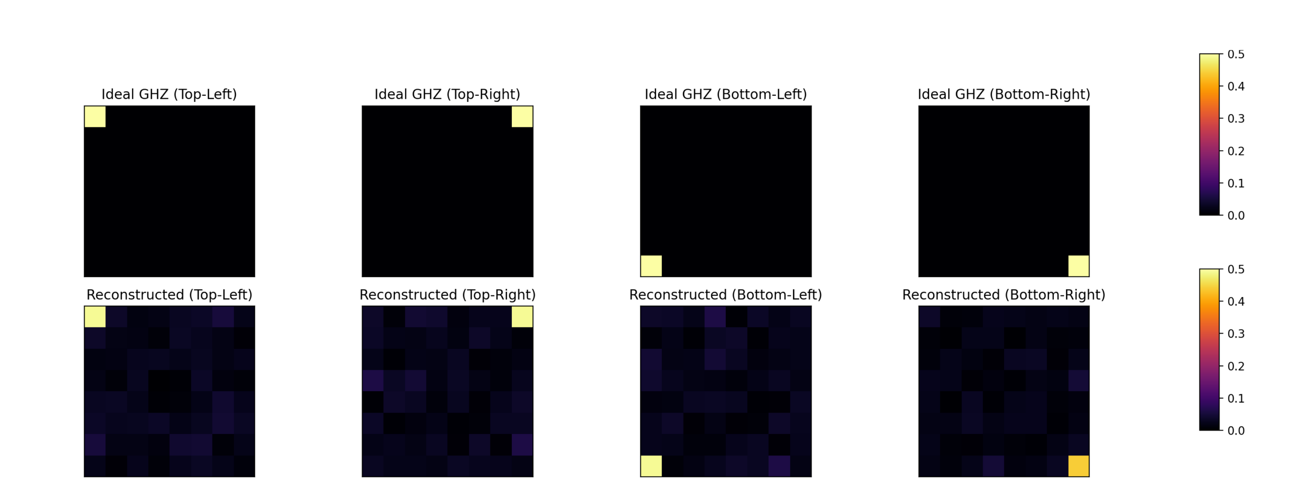
Figure 1 | Reconstruction of a 6-qubit GHZ state using classical shadows. The four corners are the density-matrix entries indexed by the all-zeros state $\left| 000000 \right\rangle$ and the all-ones state $\left| 111111 \right\rangle$ , the only two basis states appearing in the GHZ superposition. The ideal GHZ density matrix has all of its weight in these four entries, where the two diagonal corners gives the populations and the two off-diagonal corners gives the coherences. The top row shows these ideal corners, and the bottom row shows the reconstructed estimate from randomized measurements.

Figures 2 and 3 are also based on the same 6-qubit GHZ state. Figure 2 shows trace-distance reconstruction error versus number of measurement shots on a log-log scale. Figure 3 shows fidelity estimates across many trajectories.

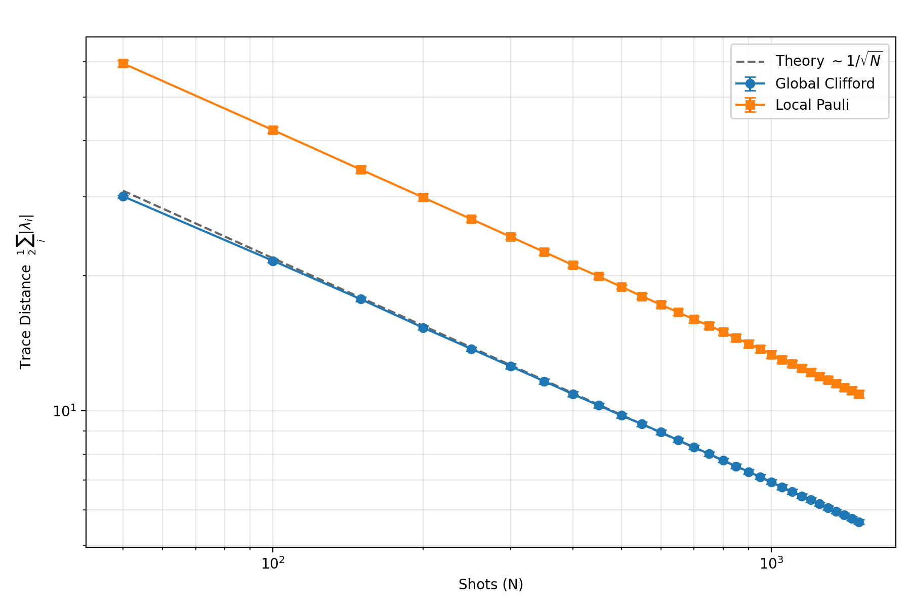
Figure 2 | Trace-distance reconstruction error versus number of measurement shots on a log-log scale for a 6-qubit GHZ state. The two curves compare local Pauli and global Clifford measurements. Both show roughly $\frac{1}{\sqrt{N}}$ behavior, where $N$ is the number of shots.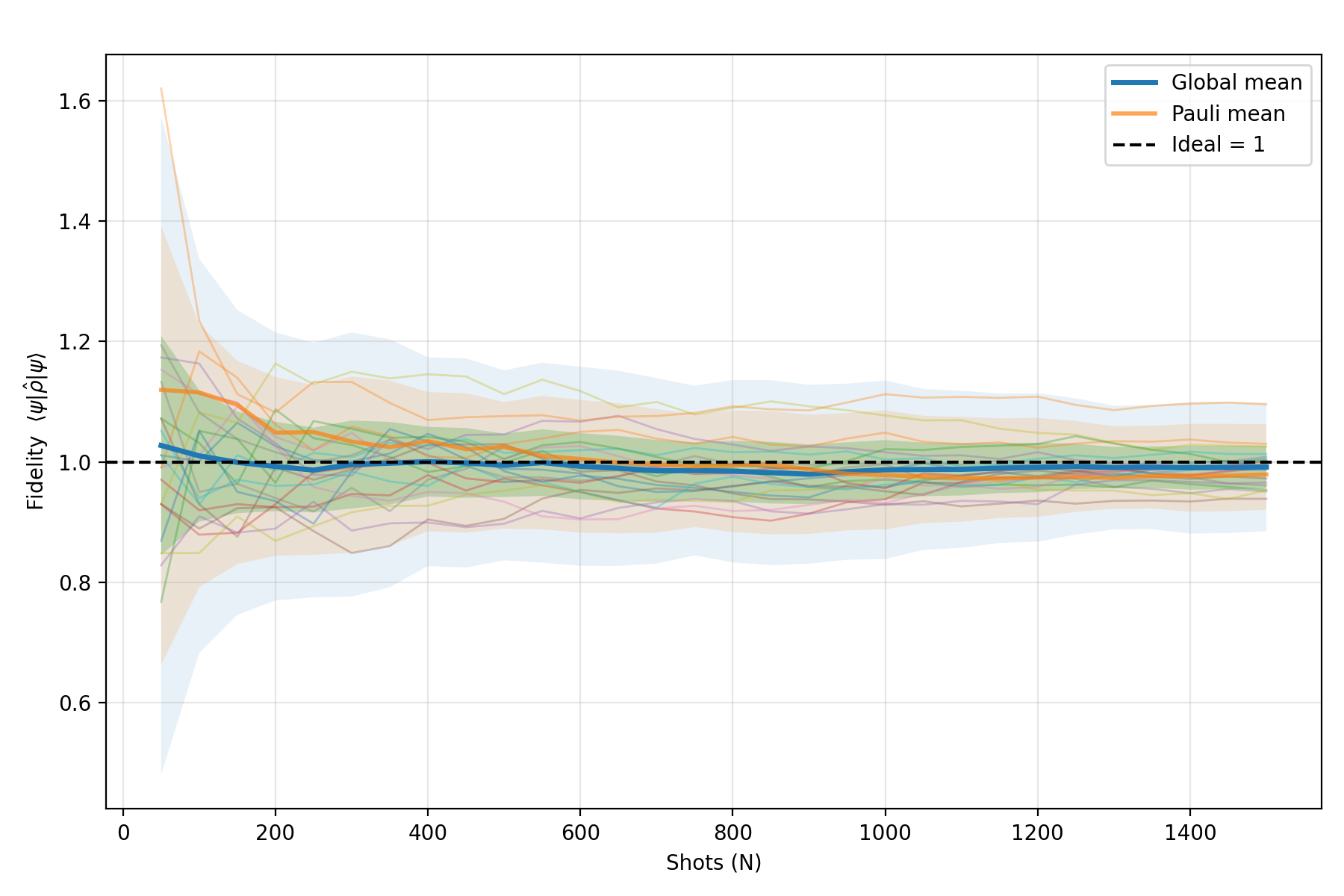

Figure 3 | Fidelity versus number of measurement shots for a 6-qubit GHZ state across multiple trajectories. The spread gets smaller as more shots are used.

Figure 4 shows purity estimation on the same 6-qubit GHZ state. Here purity means $Tr\left( \rho^{2} \right)$ . Unlike the witness expectation value later in the paper, this is not linear in $\rho$ , which is one reason it is harder to estimate.

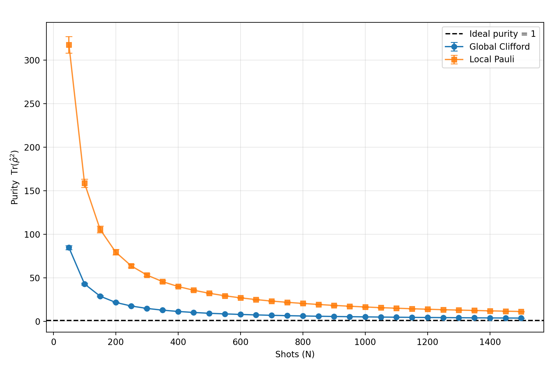Figure 4 | Purity estimation for a 6-qubit GHZ state versus number of measurement shots. Here purity means $Tr\left( \rho^{2} \right)$ , which is nonlinear in $\rho$ . Compared with linear observables, the estimator has larger spread, especially at smaller shot counts.

These benchmark plots serves as preliminary checks that the shadow estimators behave as expected in a known entangled-state setting. The main claims of the paper are tested in the witness experiments below. The observable being estimated in these experiments is the Bell witness itself rather than a general reconstruction metric.

Main Results

Witness estimation accuracy

In an actual witness problem, we are not interested in a generic reconstruction metric, and we care about the witness itself.

So in the rest of the paper, we move from general shadow benchmarks to a witness-based example. We pick the Bell state to be our entangled state because it is the simple and its witness can be written exactly in Pauli form.

We take the Bell state

$|\Phi^{+}\rangle = \frac{|00\rangle + |11\rangle}{\sqrt{2}}.$

A standard projector-form witness for this state is⁷.

$W = \alpha I - |\Phi^{+}\rangle\langle\Phi^{+}|,\ \ \alpha = \frac{1}{2}$

Here $\alpha = \frac{1}{2}$ is chosen because it is the maximum possible overlap between the Bell state $|\Phi^{+}\rangle$ and any separable two-qubit state. In other words,

$\max_{\sigma \in SEP}{Tr}\left( \sigma\left| \Phi^{+}\rangle\langle\Phi^{+} \right| \right) = \frac{1}{2}$

Therefore, for every separable state $\sigma$ ,

$Tr(W\sigma) = \frac{1}{2}\ - \ Tr\left( \sigma\left| \Phi^{+}\rangle\langle\Phi^{+} \right| \right) \geq 0,$

while for the Bell state itself,

$Tr\left( W\left| \Phi^{+}\rangle\langle\Phi^{+} \right| \right) = \frac{1}{2} - 1 = - \frac{1}{2}$

Thus, $\alpha = \frac{1}{2}$ gives the tight standard witness of this projector form: increasing $\alpha$ would still give a valid witness but would make the violation weaker, while decreasing $\alpha$ would make the operator negative on some separable states. Using the Pauli decomposition of the Bell projector,

$|\Phi^{+}\rangle\langle\Phi^{+}| = \frac{1}{4}(II + XX - YY + ZZ),$

the witness becomes

$W = \frac{1}{4}(II - XX + YY - ZZ).$

Its non-identity terms act on two qubits, so the witness locality is $m = 2$ .

Our first witness experiment asks a statistical question. With the implementation of classical shadows for estimating Bell witnesses, how will the error vary with the increasing number of shadows? To calculate the error of estimation, the following formula is used:

$\left| \widehat{Tr(W\rho)} - Tr(W\rho) \right|,$

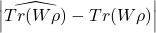
where $\widehat{Tr(W\rho)}\$ is the median-of-means value obtained from the samples and Tr(W $\rho$ ) is the actual value. The plotted figure represents the average absolute error over 100 times run. Furthermore, the error bars represent the standard deviation.

To achieve this, we fix the Bell state, calculate $Tr(W\rho)$ , and then compare the result with the correct figure. The procedure uses both local Pauli measurements and global Clifford measurements. We implement the median-of-means (MoM) method using 4 different groups. The output of a single-shot estimate is then divided into 4 sets, and a mean for each subset is calculated. Finally, the values used to obtain MoM will present the final estimate as the median of means. This is the same way traditional classical shadows works because median-of-means is used to obtain high-probability estimates, whereas sample complexity theory for classical shadows assumes that one needs to take multiple groups of shadow estimates and perform a median on the results to account for extreme outlier effects. The common mean is sensitive to outlier snapshots, while median-of-means tends to be more reliable since one noisy group will have a weaker influence on the final estimate. For the majority of calculations, we use 4 groups of estimates. In the embedding experiment, we increase this number to 8 since we still leave 25 sample estimates meaning that we perform much more reliable estimation.

Mean absolute errors depicted in Figure 5 are plotted against different shadow counts. In this scenario, the median of means method has been utilized. The decay observed is compared to the expected behavior by plotting the mean absolute error in log-log scale. The fitted exponent for the local Pauli measurements is found to be -0.4760, with a 95% bootstrap confidence interval of [-0.5640, -0.3901]. In case of global measurements, the exponent is found to be -0.5496, with a 95% bootstrap confidence interval of [-0.6362, -0.4641]. Both of the measured exponent values are quite similar to the reference value of -1/2. Further, the measuring exponents imply that by increasing the number of shadows to double, the mean absolute error is reduced by a factor of around $2^{- 0.4760} \approx 0.72$ for local Pauli measurements and $2^{- 0.5496} \approx 0.68$ for global measurements. This is quite close to the ideal reduction of $1/\sqrt{2} \approx 0.71$ expected from inverse-square-root scaling.

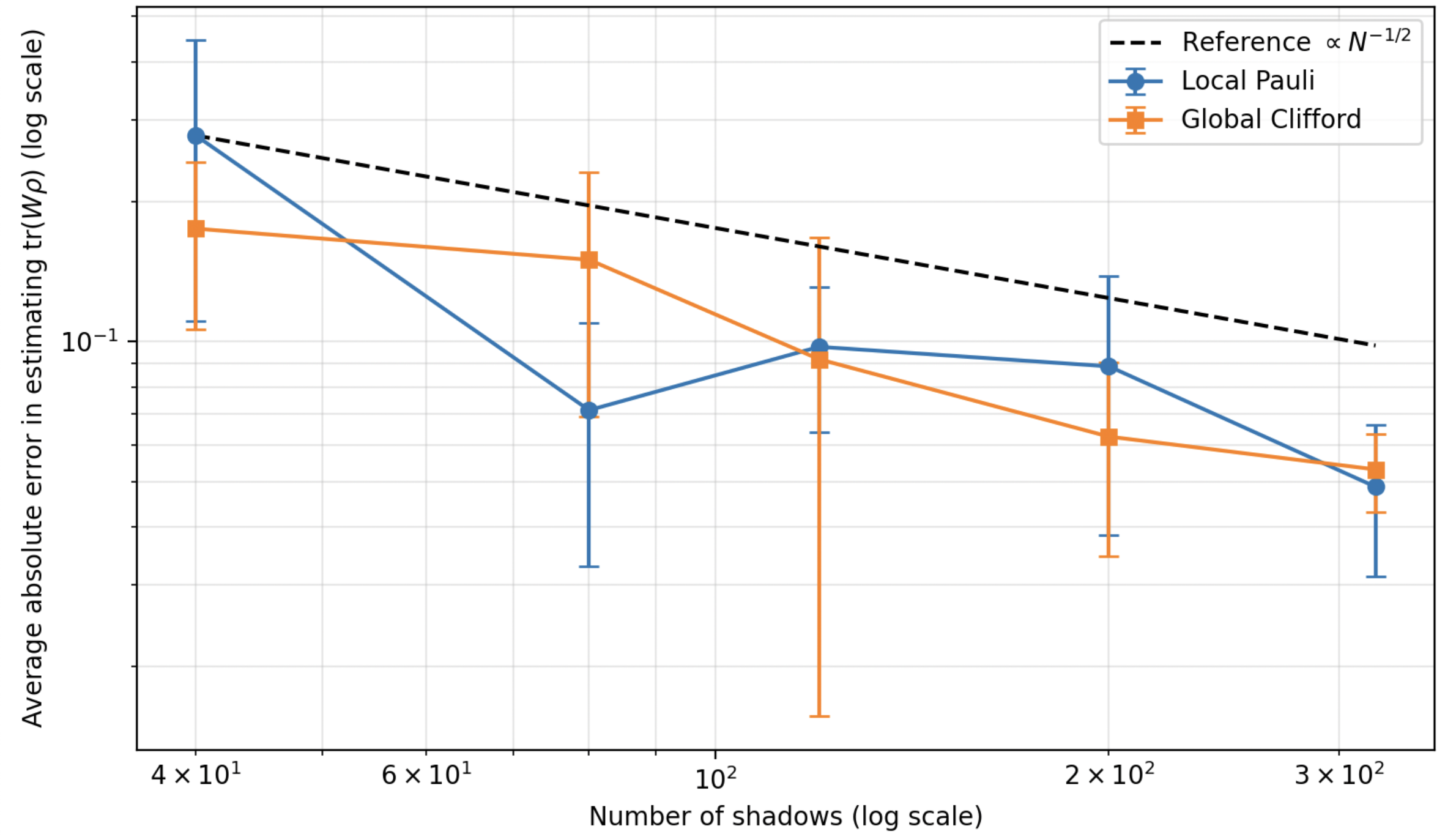
Figure 5 | Bell witness estimation error versus number of shadows. The vertical axis indicates the mean absolute error $\left| \widehat{Tr(W\rho)} - Tr(W\rho) \right|$ over 100 repetitions whereas error bars show standard deviation over repetitions. We measure $Tr(W\rho)$ of the Bell state through using local Pauli types and global Clifford measurements. The shadow counts utilized are 40,80,120,200,320. Each measurement is taken using the median of means of the 4 groups as one measurement. The log-log plot gives an estimate -0.4760 of the exponent for local Pauli and -0.5496 for global Clifford measurements. The dashed line shows the reference $N^{- 1/2}$ .

Figure 5 depicts the comparison of the two measurement ensembles for the same Bell-witness effort. The results show that in this experiment although the local Pauli measurements have performed at least as well as the global Clifford operators in the case of the low-locality observable. This is quite reasonable since the Bell witness consists of only a limited number of two-qubit Pauli strings and thus matches perfectly well with the local means of measurements. At the same time, global Clifford measurements are more universal and can be used for various global measurements but require more complex entangling rotations and do not guarantee any improvements in the performance of the fixed low-locality measurements.

Depolarizing noise case study

We examine the depolarizing-noise model in this initial noise test. The simplicity of this model yields a witness value that is easy to calculate and an easily recognizable threshold. It is important to realize, however, that this model is simply a controlled example, not a complete representation of realistic experimental noise. In this model, the state is noted as

$\rho(p) = (1 - p)\rho_{Bell} + p\frac{I}{4},$

where p is the noise level. When p=0, we obtain the pure Bell state. Increasing p creates a state that approaches the maximally mixed one.

The exact dashed line in Figure 5 comes from two simple calculations:

$Tr\left( W\rho_{Bell} \right) = \frac{1}{2} - 1 = - \frac{1}{2}$

and

$Tr\left( W\frac{I}{4} \right) = \frac{1}{4}Tr(W) = \frac{1}{4}$

Therefore

$Tr\left( W\rho(p) \right) & = (1 - p)Tr\left( W\rho_{Bell} \right) + p\, Tr\left( W\frac{I}{4} \right)$

$& = (1 - p)\left( - \frac{1}{2} \right) + p\left( \frac{1}{4} \right)$

$& = - \frac{1}{2} + \frac{3}{4}p$

The witness stops detecting entanglement when this quantity reaches zero, which gives $p = \frac{2}{3}$ .

In Figure 6(a), the comparison of the exact line with shadow estimates is made by using local Pauli measurements only. Each data point is created from 200 shadows and median-of-means with 4 groups. One hundred independent runs are employed to generate the plotted estimate of the average across all runs and the error bands that depict the standard deviation across runs.

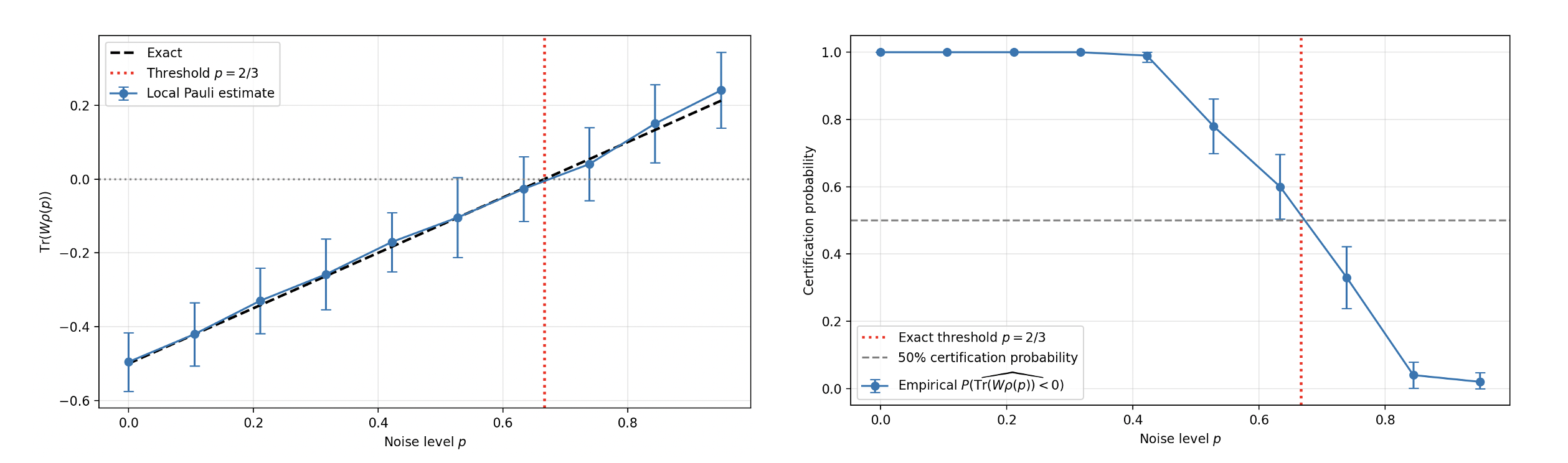
Figure 6 | Depolarizing-noise case study for the Bell witness. (a) (Left) Bell witness value for the depolarized state $\rho(p) = (1-p)\rho_{\mathrm{Bell}} + pI/4$ , using local Pauli measurements only. Each point uses 200 shots and median-of-means with 4 groups, repeated over 100 independent runs; blue points show the mean estimate, and error bars show the standard deviation across runs. The black dashed line is the exact formula $\operatorname{Tr}(W\rho(p)) = -1/2 + (3/4)p$ , and the red dotted line marks the threshold $p = 2/3$ . (b) (Right) Empirical probability of certifying entanglement, i.e., the probability that the estimated witness value is negative, from the same 100 runs. The red dotted line marks $p = 2/3$ , and the gray line marks the 50% certification level.

In order to connect finite-shot data and the entanglement certification process, Fig. 6(b) depicts the empirical likelihood that the estimator gives a negative value of the witness. For instance, the estimator is shown to be able to certify entanglement in approximately 60% of cases at about threshold $p = 0.633$ (95% confidence interval 0.504–0.696). On the other hand, at $p = 0.739\$ the probability of the certification drops to 33% and reaches only 4% at $p = 0.844$ . Thus, based on the data of 200 shadows, the estimator does not recognize the threshold point as such. Instead, there is a finite-shot transition region around $p = 2/3$ characterized by its thickness reflecting the variance of the estimator at this number of shots.

The research shows that the shadow estimator can get the right value of the witness in the symmetric depolarizing model, revealing its expected properties. However, this does not mean that the shadow estimator can be considered generally robust against realistic noise. Other noise channels, such as local dephasing, amplitude damping, failure in state preparation, or measurement process, will influence the value of the witness and certification threshold in dissimilar ways.

System-size independence of local witnesses

Local Pauli shadows makes the cost of the Bell witness depend only on locality rather than the number of qubits. To investigate this, we show the Bell witness in the n-qubit scenario in Figure 7:

$W_{embed} = W \otimes I_{n - 2}.$

We define a specific Bell state for the first two qubits, with the other qubits at 0. Also, we create an observable with the same locality

$W_{embed} + \epsilon Q,$

where

$Q = XZ \otimes I_{n - 2},\quad\quad\epsilon = 0.08.$

This $\epsilon = 0.08$ was hand-picked to make the perturbation more visible while still staying in a small-perturbation regime. Since $Q$ acts only on the same two qubits, the locality stays at $m = 2$ .

Now we explain the exact dashed lines in Figure 6. Since the state factorizes as

$\rho = \rho_{Bell} \otimes \left| 0 \right\rangle\left\langle 0 \right|^{\otimes (n - 2)},$

we have

$\begin{aligned}Tr\left( \rho W_{embed} \right) & = Tr\left( \rho_{Bell}W \right)Tr\left( \left| 0 \right\rangle\left\langle 0 \right|^{\otimes (n - 2)}I_{n - 2} \right) \& = Tr\left( \rho_{Bell}W \right) \& = - \frac{1}{2}\end{aligned}$

So the exact value of $Tr\left( \rho W_{embed} \right)$ does not depend on $n$ .

For the perturbed observable,

$Tr\left( \rho\left( W_{embed} + \epsilon Q \right) \right) = Tr\left( \rho W_{embed} \right) + \epsilon\, Tr(\rho Q).$

Here $Tr(\rho Q) = \left\langle \Phi^{+}|XZ|\Phi^{+} \right\rangle = 0$ , so $Tr\left( \rho\left( W_{embed} + \epsilon Q \right) \right) = - \frac{1}{2}$ . The two exact dashed lines overlap each other for this reason. Thus, we should not consider this perturbation to be an evaluation of sensitivity to a modified value of the true witness. Instead, it tests whether adding a same-support Pauli term changes the estimator fluctuations while leaving the exact mean fixed.

The estimated witness values are presented in Figure 7 as the system size n changes from 3 to 6. The measurement is based on a fixed value of 200 shadows for each value we obtain. The process is referred to as median-of-means, which represents that the 8 groups are used. The number of groups is determined in accordance with the median-of-means approach with regard to the sample-complexity theorem of classical shadows.

We would like to point out that the perturbed operators we will be using below should not be interpreted as valid entanglement witnesses. The original Bell witness W as such is a valid witness but adding Pauli perturbations such as $\epsilon Q$ or $\epsilon R$ destroys the condition of the operator being nonnegative on all separable states. Therefore, the perturbation experiments should be treated as observable-estimation experiments studying locality and estimator variance.

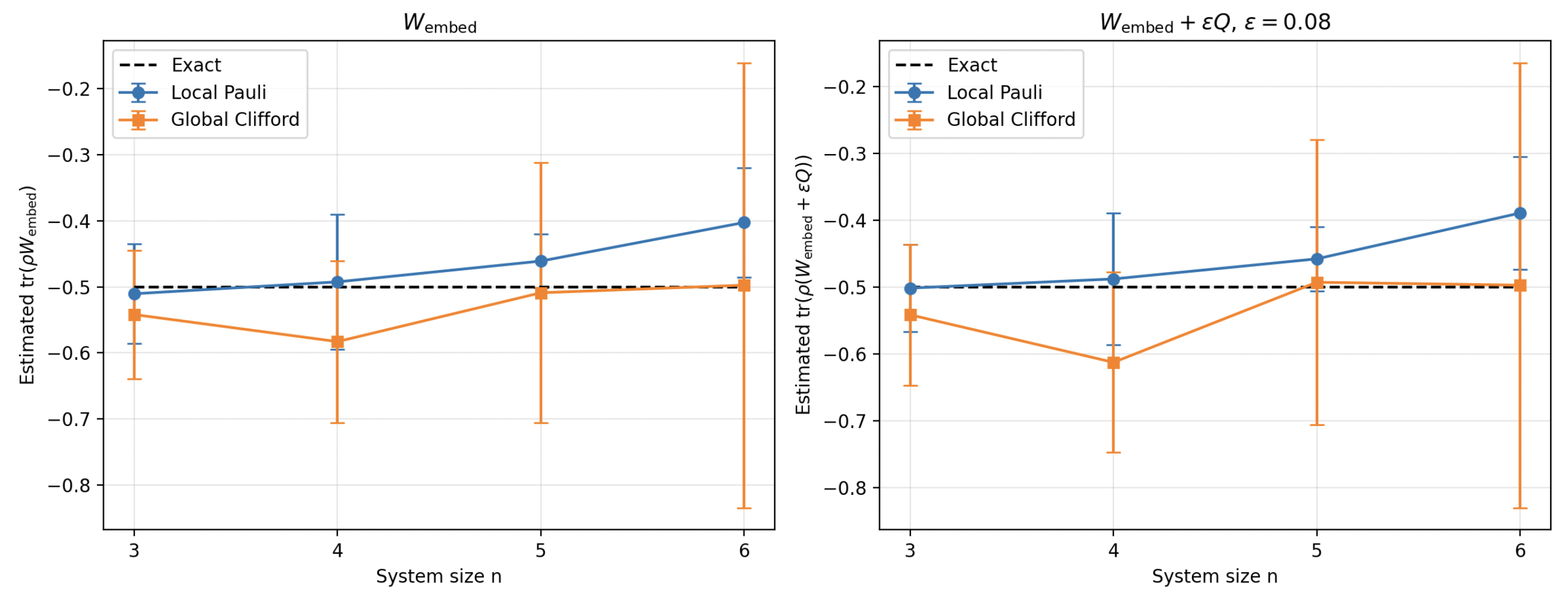
Figure 7 | Embedded Bell witness in larger systems. Here, the Bell state occupies the first two qubits and the witness acts as $W_{embed} = W \otimes I_{n - 2}$ . Furthermore, in this figure, we present the same-locality perturbed observable $W_{embed} + \epsilon Q$ with $Q = XZ \otimes I_{n - 2}$ and hand-picked $\epsilon = 0.08$ . The size of the systems under consideration varies from n=3 to n=6. The points are plotted using a fixed total number of shadows equal to 200 and the method of median-of-means with 8 groups. Both local Pauli and global Clifford panels have been used. The exact dashed lines are independent of $n$ because the witness support stays fixed and because $Tr(\rho Q) = 0$ . The perturbation being shown in this figure is meant to analyze fluctuations in the estimate rather than the influence of a change in the corresponding exact value of the witness.

The local Pauli estimation remains almost unchanged as the n parameter varies, unlike the global Clifford estimation that seems to have high variability under these conditions. This shows that even though global Clifford measurements are more complex to perform, they are of no clear advantage in relation to Bell-witness observable with fixed support.

The next step is to investigate whether the number of shots needed to collect shadows changes. In order to evaluate this aspect, we calculate the empirical variance of $Tr\left( O\widehat{\rho} \right)$ for every system size n. In this analysis we use local Pauli measurements only, as calculating shadows based on them is the most straightforward case. The analysis is performed by collecting an empirical average from 1000 shadows obtained by performing the experiment 10 times for every n parameter. The number of shots required for the additive error of 0.05 is computed from the empirical variance via formula $N_{needed} \approx Var/{0.05}^{2}$ .

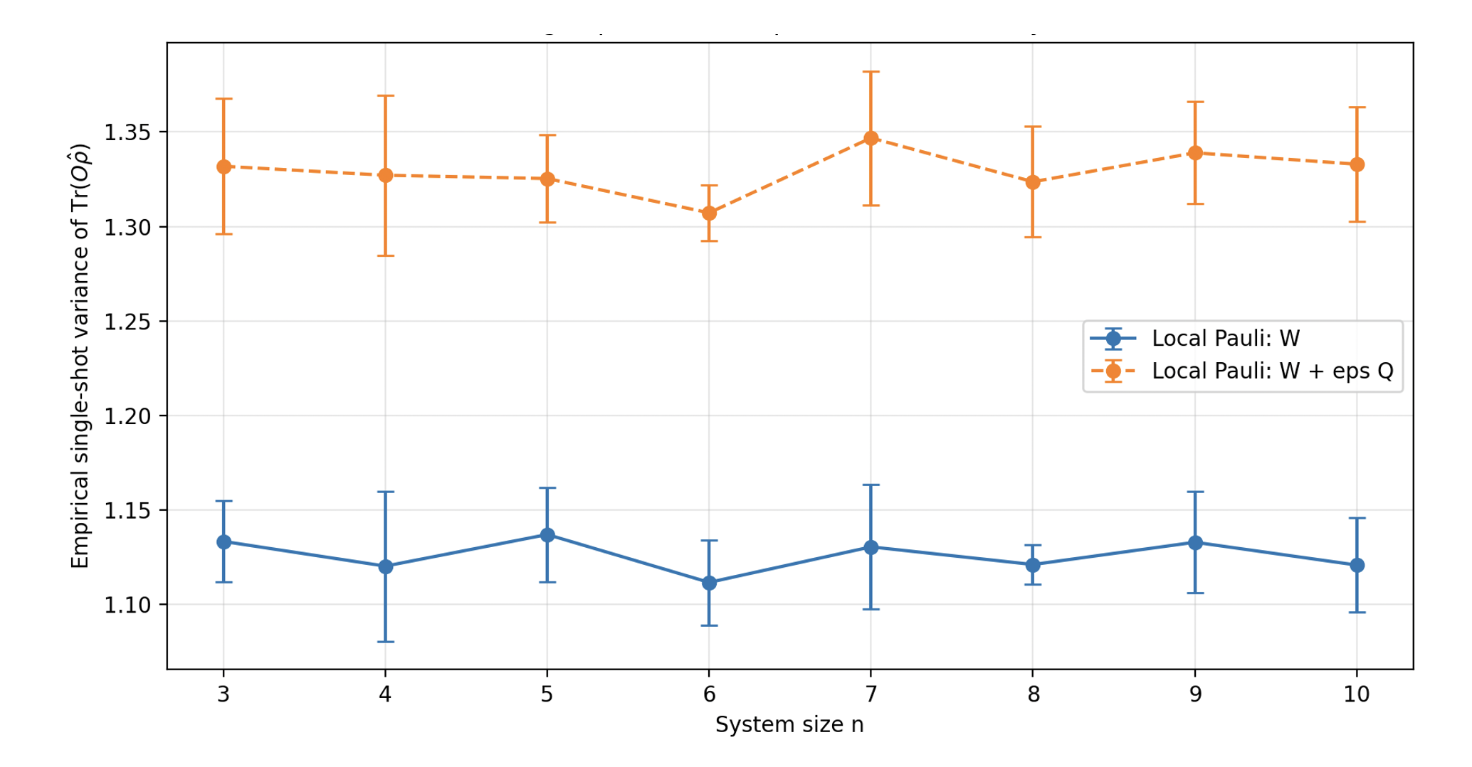
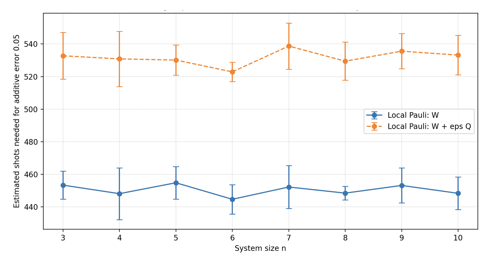Figure 7 (a) and (b) | The empirical variance and estimated shot number for the embedded Bell witness when the system size increases. (a) The empirical variance for single shots of $W_{embed} + \epsilon Q$ when using local Pauli measurement. (b) The estimated shots to get additive precision of 0.05 based on the empirical variance. For $n=3$ to $n=6$ , both parameters remain approximately constant, as this indicates that using extra qubits does not significantly affect the local Pauli measurement cost in the case of this Bell witness with constant support.

The combination of Figure 7 with the other variance evaluations indicates that in the case of the Bell witness example with a fixed support, changing the size of the whole system does not not lead to significant changes in the obtained mean value or local Pauli variance. The same is valid in relation to the estimated number of shots needed for additive error 0.05 since it also remains almost unchanged when changing n from 3 to 6. Because the perturbation Q has the zero mean related to the target state, this experiment is primarily aimed at testing the changes of the estimators depending on the local perturbation rather than testing their sensitivity to the actual change in the mean value of the witness.

Operator locality perturbation analysis

The last experiment provides a restricted evaluation of the effects of adding a support on the estimate in this Bell state case. By perturbation experiments, we are referring to the following: instead of only estimating the initial witness, we perform small modifications on the witness operator and verify how the estimates change in this context. Here the important distinction is whether the perturbation keeps the same locality or increases the support by one qubit.

We study two types of perturbations:

a same-locality perturbation, which keeps the support on the original two qubits:

$Q = XZ \otimes I_{n - 2},$

a higher-locality perturbation, which extends the support to one extra qubit:

$R = XZX \otimes I_{n - 3}.$

Therefore, the second perturbation increases locality from m=2 to m+1=3 as we have previously commented. The idea here should be interpreted only as a limited k=2 versus k=3 comparison within the Bell state study we have undertaken. This does not represent a true numerical verification of the $3^{k}$ law of scaling for many locality values. While one expects the shadow norm, and hence variance, to increase with the growing support due to local Pauli shadows, because we have a single Bell state target and make perturbations with zero expectation on that target, it should rather be seen as a limited case study of the estimator variance rather than a comprehensive test of high-locality witnesses.

In order to relate this area of locality to the shadow-norm framework, we now calculate a local-Pauli shadow-norm proxy for the actual observables that we used in the perturbation experiments. Suppose that we have an observable that can be expressed in a Pauli expansion $O = \sum_{P}c_{P}P$ , we have

$\sum_{P}c_{P}^{2}3^{w(P)},$

such that we denote $w(P)$ as the Pauli weight. Although this quantity is not a true state-dependent variance, it still captures the standard local-Pauli cost connected to the operator support. Further, we compare this proxy with empirical single-shot variance of $Tr\left( O\widehat{\rho} \right)$ which is calculated through 5000 shadow samples.

Observable	Locality	Theory proxy	Local Pauli variance	Global Clifford variance
$W$	2	1.75000	1.11116	3.36992
$W + \epsilon Q$	2	1.80760	1.17070	3.47879
$W + \epsilon R$	3	1.92280	1.26594	3.49130

Table 1 | The relationship between the local-Pauli shadow-norm proxy and the empirical single-shot variance for the observables employed in the perturbation studies. In this case $n = 4$ , $\epsilon = 0.08$ and shadows are set to 5000.

Both the theory proxy and empirical variance show the same trend of results. It shows that the original Bell witness W has the lowest predicted and obtained costs. The same locality perturbation observable $W + \epsilon Q$ is of larger value and the higher locality perturbation observable $W + \epsilon R$ has the highest value. Thus it connects the shadow-norm talking to actual measurement results obtained in simulations, but it still remains a limited comparison in the framework of Bell state case.

Next, we explore the effects of various degrees of perturbation, $\epsilon$ , through two means:

equally spaced values,
exponentially spaced values.

While doing the operations, 200 shadows were used for every measurement point along with 4 groups for the median-of-means. In case of the Figure 8, the size of the system represented is n = 4.

The exact lines overlap in this figure because both perturbation terms have zero expectation value on the target state. More specifically,

$\left\langle \Phi^{+}|XZ|\Phi^{+} \right\rangle = 0\quad\text{and}\quad\left\langle \Phi^{+} \right|\left\langle 0 \right|XZX\left| \Phi^{+} \right\rangle\left| 0 \right\rangle = 0.$

Thus, the value comes out to be $Tr(\rho W) = - \frac{1}{2}\$ for both kinds of observable. The figure illustrates the spread of the estimator, but not the shift in the mean value. This indicates that the figure cannot be taken as an evidence to claim that higher locality witnesses will behave similarly.

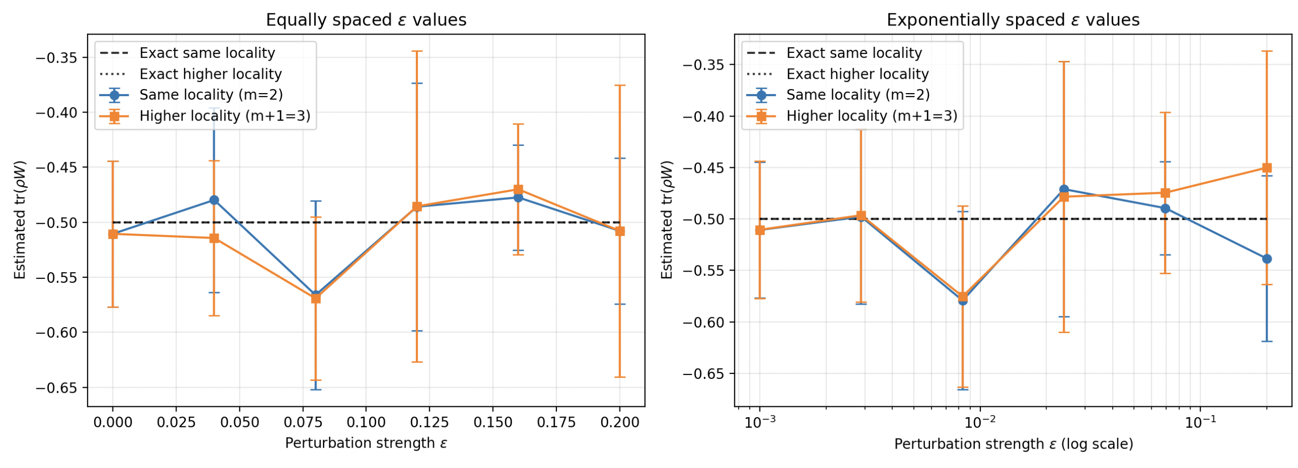Figure 8 | Perturbation study for same-locality and higher-locality observables in a 4-qubit system. The left image has an equally spaced $\epsilon$ values, while the right section contains exponentially spaced $\epsilon$ values. Both sections make use of local Pauli measurements only, with a fixed 200 shadows and median-of-means having 4 groups. The same-locality perturbation is $Q = XZ \otimes I_{n - 2}$ and the higher-locality perturbation is $R = XZX \otimes I_{n - 3}$ . The exact lines overlap because both perturbation terms have zero expectation value on the target state.

According to our data, the two underlying curves overlap a lot in the specific range of epsilon studied. This indicates that at least for these perturbations and for the given budget, the increase from 2 to 3 does not significantly change the plot of estimator variance. However, this is a weak evidence for the locality-scaling statement since both perturbations have zero expectation with respect to the target state and we use only one example of the Bell state. Future work should check perturbations with nonzero expectations, different target states and more complicated sets of high locality observables.

Finally, we return to the number of shadows, but instead of plotting error, we plot the estimated observable value itself. We compare $Tr(\rho W)$ and $Tr\left( \rho O_{pert} \right)\$ as functions of the shadow count, where $O_{pert}$ denotes the perturbed observable. We show both local Pauli and global Clifford panels. The perturbation strength is fixed at $\epsilon = 0.08$ .

As in Figures 7 and 8, the exact values overlap because the perturbation term has zero expectation on the target state. So both exact lines are at $- 1/2$ .

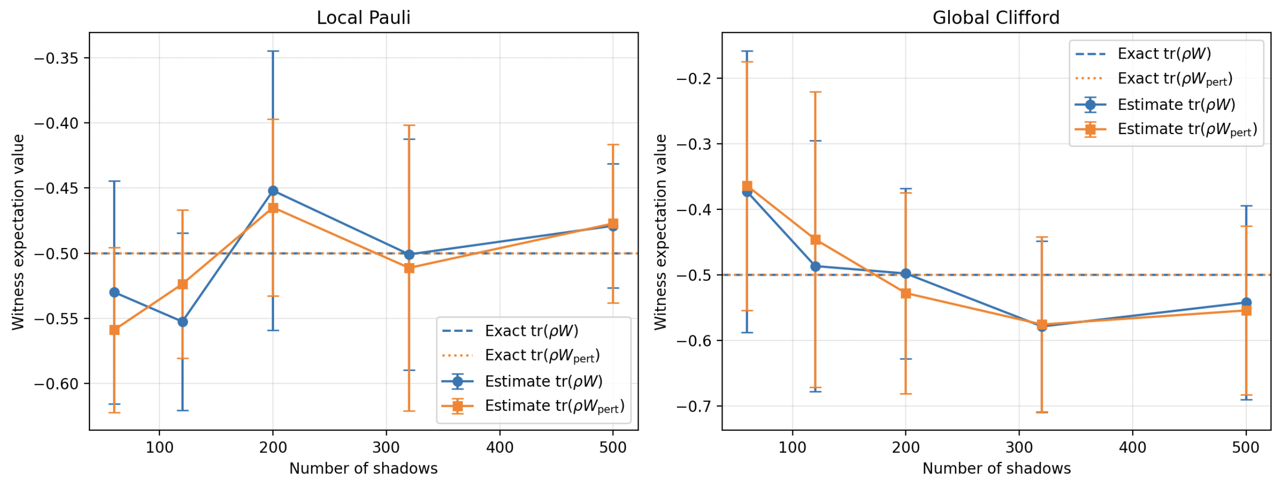Figure 9 | Estimated observable expectation values versus number of shadows for the original embedded witness and the perturbed observable with $\epsilon = 0.08$ . The left image shows local Pauli measurements, while the right column shows global Clifford measurements; the number of shadows used in this case are 60,120,200,320,500, and the median-of-means involves 4 groups.

In such situations, the local Pauli measurements are performing reasonably well because there are comparatively fewer Pauli strings formed by observables. Though the global Clifford measures are better in many respects, they do not seem to offer any clear advantages in this experiment. This allows suggesting that the measurement ensemble is dependent on the nature of the observable: local Pauli measures are suitable for low-locality Pauli measures, whereas global Clifford measures are appropriate for problems with a higher degree of global system organization.

Overall, the conducted experiments show that, in this particular case involving the Bell witness, fixed witness properties have been found to be more important than system size in deciding the estimation outcome. More broadly, the claims made for the situation involving higher locality or true multipartite witnesses would require some further experimental study.

Discussion

The results above support a more specific central idea: in the Bell witness case study considered here, the practical difficulty of estimation is closely connected to the structure and support of the observable. The GHZ plots that are displayed in the classical shadow part should be regarded as benchmarks of the methods that have been used rather than as substantiation for this locality argument. They show that the shadow estimates behave reasonably well, however, nonlinear quantities like purity are more complex to estimate. The Bell witness discussions provide the most important conclusions regarding this witness.

The first witness experiment allows understanding the behavior of witnesses on the statistical level. It can be seen that with increasing number of shadows, the absolute witness estimation error declines not only for local Pauli measurements, but also for global Clifford measurements. The log-log fit returns exponents equal to -0.4760 for local Pauli measurements and -0.5496 for global Clifford measurements, which are in accordance with the theoretical prediction $N^{- 1/2}$ scaling. In practical terms, doubling the number of shadows reduces the fitted error by a factor of about $0.72$ for local Pauli measurements and $0.68$ for global Clifford measurements, close to the ideal inverse-square-root factor $1/\sqrt{2} \approx 0.71$ .

The depolarizing-noise experiment offers witness a physical significance, but its interpretation has to be done with caution. In principle, we should be able to realize the state in an ideal experiment where it takes value $\rho(p) = (1 - p)\rho_{Bell} + pI/4$ , we witness the behavior of the estimator close to the known analytic threshold. The curve goes through zero at the point $p = 2/3$ , whereas the finite-shot estimator illustrates a smooth transition around this value. Therefore, after measuring the state with 200 shadows, we can see the qualitative behavior of the threshold in the experiment, but it would not be possible to estimate its location accurately.

The embedding experiment addresses the main statistical scaling question. The embedding of the Bell witness in a larger system comprised of n qubits leads to a great expansion of the Hilbert space, but still only the first two qubits will be affected by the witness. It means that the crucial value of the witness won’t change. The variance analysis performed in this paper supports this idea and shows that the results of empirical single-shot variance and the number of shots needed for additive error equal to 0.05 are almost constant when n changes from 3 to 6. This is the reason why it can be claimed that witness support is more important in terms of statistical cost than system size in the case of Bell witness examined in this paper. Nevertheless, not all practical costs will be independent of n. Thus, classical memory, bookkeeping, state initialization, circuit execution, and mainly the creation of global Clifford unitaries may become more expensive when the number of qubits increases.

The perturbation experiments should be interpreted more carefully. The same-locality perturbation Q and the higher-locality perturbation R were chosen so that their expectation values on the target state are zero. The result of this selection is that in the Figures 8 and 9 we actually compare two expected values meanwhile the essence of the term of the perturbation is that it causes perturbations in the measurement result but does not allow shifting the expected value itself. Taking into account the overlapping of two types of the perturbation gives evidence for robustness of this witness for the type of experiments under consideration, still it cannot be considered as a proof of robustness for all other types of perturbations.

One limitation associated with the current study is that the primary witness instance is still that of a Bell witness, which is a simple two-qubit situation. Although the present study may extend this witness to larger scenarios, the nontrivial operator’s support remains stuck on two qubits. Thus, the experiments therefore do not yet cover genuinely multipartite witnesses, or families of witnesses with systematically increasing locality. Specifically, the present study relies on the $3^{k}$ local-Pauli scaling approach as a theoretical background, however it does not get to the point of doing a numerical analysis over many values of k. Another limitation is because perturbation terms were chosen to have zero expectation on the desired state. Thus, for future experiments we suggest perturbations that will affect the witness value. Another limitation is the number of qubits in numerical experiments which were restricted to using Bell states of two qubits, GHZ benchmark of 6 qubits and Bell witnesses embedded in systems of $n = 6$ , that is why the link to bigger quantum devices is motivational only.

In conclusion, the findings propose a rule of thumb for employing classical shadows in entanglement verification: the witnesses used in the process should ideally have low support. While a low-locality witness remains valid in a larger quantum system, increasing support leads to an increase in shadow norm, thus requiring many more measurements. The results also highlight the need for further developments in creating or devising the use of witnesses of entanglement that are not only mathematically correct but also efficient in statistical estimation.

Conclusion

The conceptual conclusion drawn from this article is rather straightforward. In the case of the Bell witness experiments reviewed in this article, it appears that the primary statistics depend more on the witness support and less on the total Hilbert space dimension. A witness with small support can be still statistically useful even when being part of a larger system. In the course of our limited perturbative analysis, it was discovered that the increase in the witness support from 2 to 3 qubits only led to a minor increase in the expected shadow-norm proxy and empirical variance but did not create any significant change in the behavior of the estimators.

$N = O\left( \frac{\parallel O \parallel_{sh}^{2}}{\varepsilon^{2}}\log\frac{1}{\delta} \right),$

since increasing witness support typically increases the shadow norm and therefore the required number of measurements.

The Bell state example provides a good illustration of the idea. The error of the estimator diminishes as the shot number increases, the cases of depolarizing noise are in accordance with the expected threshold for symmetric noise model $p = \frac{2}{3}$ , and the embedding experiment proves that the situation with fixed-support witnesses is manageable despite the increase in system size. Accordingly, the perturbation analysis should be understood more restrictively; this comparison of estimating processes has been made on the same Bell state but concerning different observables of support size, where the disturbances applied to entanglement witnesses do not demonstrate their entanglement characterization for more complex observables.

It is natural to consider families of witnesses in situations where perturbation leads to changes in the actual estimation value so that the distinction between the original witness and the perturbed observable is manifested not only in the variance of estimators but also in the mean itself. Another interesting avenue emerges from the discrepancies we have found between different estimation techniques. Such discrepancies indicate that, in fact, there can be an essential difference in the interaction between the measurement ensemble and the witness, especially when the support of the witness begins to expand. Studying the cases in more detail can allow us to understand where local Pauli measurements start to behave differently from global Clifford measurements in a reasonable way. Another possible line of research is to go beyond fixed analytic witnesses and find some algorithms that would allow using shadow data for generating or modifying witness in a regular manner²⁴^,²⁵^,²⁶^,²⁷. The present research does not include this adaptive process; instead, all methodologies that will be applied in this work were chosen manually, thereby giving the opportunity to examine the behavior of the shadow method in a strict experimental setting. In the future, one of the biggest projects would be to study fixed and growing observables when examining experimental or simulated systems based on 20, 50 or even more qubits, where it would be much more evident what is the difference between the cost of statistical measurements and associated resource requirements, respectively.

References

M. A. Nielsen, I. L. Chuang. Quantum computation and quantum information. Cambridge University Press, 2010. [↩]
M. A. Nielsen, I. L. Chuang. Quantum computation and quantum information. Cambridge University Press, 2010. [↩]
P. W. Shor. Polynomial-time algorithms for prime factorization and discrete logarithms on a quantum computer. SIAM Journal on Computing. Vol. 26, pg. 1484–1509, 1997, https://doi.org/10.1137/S0097539795293172. [↩]
A. K. Ekert. Quantum cryptography based on Bell’s theorem. Physical Review Letters. Vol. 67, pg. 661–663, 1991, https://doi.org/10.1103/PhysRevLett.67.661. [↩]
V. Giovannetti, S. Lloyd, L. Maccone. Advances in quantum metrology. Nature Photonics. Vol. 5, pg. 222–229, 2011, https://doi.org/10.1038/nphoton.2011.35. [↩]
B. M. Terhal. Bell inequalities and the separability criterion. Physics Letters A. Vol. 271, pg. 319–326, 2000, https://doi.org/10.1016/S0375-9601(00)00401-1. [↩]
O. Gühne, G. Tóth. Entanglement detection. Physics Reports. Vol. 474, pg. 1–75, 2009, https://doi.org/10.1016/j.physrep.2009.02.004. [↩] [↩]
M. Bourennane, M. Eibl, C. Kurtsiefer, S. Gaertner, H. Weinfurter, O. Gühne, P. Hyllus, D. Bruß, M. Lewenstein, A. Sanpera. Experimental detection of multipartite entanglement using witness operators. Physical Review Letters. Vol. 92, pg. 087902, 2004, https://doi.org/10.1103/PhysRevLett.92.087902. [↩]
H.-Y. Huang, R. Kueng, J. Preskill. Predicting many properties of a quantum system from very few measurements. Nature Physics. Vol. 16, pg. 1050–1057, 2020, https://doi.org/10.1038/s41567-020-0932-7. [↩] [↩] [↩] [↩]
A. Elben, S. T. Flammia, H.-Y. Huang, R. Kueng, J. Preskill, B. Vermersch, P. Zoller. The randomized measurement toolbox. Nature Reviews Physics. Vol. 5, pg. 9–24, 2023, https://doi.org/10.1038/s42254-022-00535-2. [↩]
S. Aaronson. Shadow tomography of quantum states. Proceedings of the 50th Annual ACM SIGACT Symposium on Theory of Computing, pg. 325–338, 2018 [↩]
D. E. Koh and S. Grewal. Classical shadows with noise. Quantum. Vol. 6, pg. 776, 2022, https://doi.org/10.22331/q-2022-08-16-776. [↩]
K. Bu, D. E. Koh, and A. Jaffe. Classical shadows with Pauli-invariant unitary ensembles. npj Quantum Information. Vol. 10, Article 6, 2024, https://doi.org/10.1038/s41534-023-00801-w. [↩]
M. Ippoliti. Classical shadows based on locally-entangled measurements. Quantum. Vol. 8, pg. 1293, 2024, https://doi.org/10.22331/q-2024-03-21-1293. [↩]
B. Vermersch, A. Rath, B. Sundar, C. Branciard, J. Preskill, and A. Elben. Enhanced estimation of quantum properties with common randomized measurements. PRX Quantum. Vol. 5, pg. 010352, 2024, https://doi.org/10.1103/PRXQuantum.5.010352. [↩]
A. Seif, Z.-P. Cian, S. Zhou, S. Chen, and L. Jiang. Shadow distillation: quantum error mitigation with classical shadows for near-term quantum processors. PRX Quantum. Vol. 4, pg. 010303, 2023, https://doi.org/10.1103/PRXQuantum.4.010303. [↩]
H. Jnane, J. Steinberg, Z. Cai, H. C. Nguyen, and B. Koczor. Quantum error mitigated classical shadows. PRX Quantum. Vol. 5, pg. 010324, 2024, https://doi.org/10.1103/PRXQuantum.5.010324. [↩]
H.-Y. Hu, A. Gu, S. Majumder, H. Ren, Y. Zhang, D. S. Wang, Y.-Z. You, Z. Minev, S. F. Yelin, and A. Seif. Demonstration of robust and efficient quantum property learning with shallow shadows. Nature Communications. Vol. 16, Article 3023, 2025, https://doi.org/10.1038/s41467-025-57349-w. [↩]
N. Wyderka, A. Ketterer, S. Imai, J. L. Bönsel, D. E. Jones, B. T. Kirby, X.-D. Yu, and O. Gühne. Complete characterization of quantum correlations by randomized measurements. Physical Review Letters. Vol. 131, pg. 090201, 2023, https://doi.org/10.1103/PhysRevLett.131.090201. [↩]
Y. Zhou and Z. Liu. A hybrid framework for estimating nonlinear functions of quantum states. npj Quantum Information. Vol. 10, Article 62, 2024, https://doi.org/10.1038/s41534-024-00846-5. [↩]
Z. Webb. The Clifford group forms a unitary 3-design. Quantum Information and Computation. Vol. 16, pg. 1379–1400, 2016, https://doi.org/10.48550/arXiv.1510.02769. [↩] [↩]
H. Zhu. Multiqubit Clifford groups are unitary 3-designs. Physical Review A. Vol. 96, pg. 062336, 2017, https://doi.org/10.1103/PhysRevA.96.062336. [↩] [↩]
D. Gottesman. The Heisenberg representation of quantum computers. arXiv preprint quant-ph/9807006, 1998, https://doi.org/10.48550/arXiv.quant-ph/9807006. [↩]
A. Dimić, B. Dakić. Single-copy entanglement detection. npj Quantum Information. Vol. 4, pg. 11, 2018, https://doi.org/10.1038/s41534-017-0055-x.I [↩]
V. Saggio, B. Daryanoosh, S. Paesani, A. Santagati, J. Wang, N. Wiebe, J. C. F. Matthews, A. Laing. Experimental few-copy multipartite entanglement detection. Nature Physics. Vol. 15, pg. 935–940, 2019, https://doi.org/10.1038/s41567-019-0550-4. [↩]
A. Neven, J. Carrasco, V. Vitale, C. Kokail, A. Elben, M. Dalmonte, P. Zoller, B. Vermersch. Symmetry-resolved entanglement detection using partial transpose moments. npj Quantum Information. Vol. 7, pg. 152, 2021, https://doi.org/10.1038/s41534-021-00487-y. [↩]
Y. Zhou, P. Zeng, Z. Liu. Single-copies estimation of entanglement negativity. Physical Review Letters. Vol. 125, pg. 200502, 2020, https://doi.org/10.1103/PhysRevLett.125.200502. [↩]

Abstract

Introduction

Classical Shadow Tomography

Main Results

Witness estimation accuracy

Depolarizing noise case study

System-size independence of local witnesses

Operator locality perturbation analysis

Discussion

Conclusion

References

RELATED ARTICLESMORE FROM AUTHOR

ADHD Musicians Show Distinct Pathways from Stimulation to Well-Being in a Large-Scale Study

Creating Natural Paint Through Gardenia Fruit Extraction

Accessible VQA Evaluation Using Reading-Level Controlled GQA

LEAVE A REPLY Cancel reply

RELATED ARTICLES MORE FROM AUTHOR