Detecting Chaos in Stock Markets: Non-linear Dynamics in a Developed (the UK) and a Developing (India) Economy

Abstract

This research investigates whether the daily price movements of a major developed-market stock index (FTSE-100 in the UK) and a major emerging-market stock index (BSE-SENSEX in India) display nonlinear and chaotic-like behaviour, as indicated by the largest Lyapunov exponent (LE). The LE quantifies the average exponential rate at which nearby trajectories in a dynamical system’s phase space diverge or converge, with positive values indicating sensitive dependence on initial conditions, a key feature of chaos. Using daily closing prices for the FTSE-100 and BSE-SENSEX from January 2001 to 2025, phase space reconstruction was performed using Takens’ embedding theorem, with optimal time delay estimated by the mutual information function and the embedding dimension determined by the false nearest neighbours algorithm. For the log differenced (stationary) series, the BSE-SENSEX yielded a larger positive LE (λ = 0.1513) than the FTSE-100 (λ = 0.0212), denoting a faster trajectory divergence and comparatively stronger non-linear dynamics in the emerging market. Both raw price series exhibited similar positive LEs (FTSE-100: 0.1602; BSE-SENSEX: 0.1614). These differences may reflect structural distinctions between developed and developing markets, including liquidity, regulatory maturity, information asymmetry, and investor composition. However, a positive LE alone is not proof of deterministic chaos, as stochastic processes can produce similar results. The LE is therefore interpreted as a descriptive, comparative indicator. For policymakers and market participants, these outcomes challenge the widely held assumption that stock price movements are purely stochastic and suggest that linear models alone may be insufficient for assessing market stability and risk.

Keywords: chaos theory, Lyapunov exponent, nonlinear dynamics, phase-space reconstruction, stock market, FTSE-100, BSE-SENSEX, emerging markets, developed markets, Taken’s embedding theorem

Introduction

Chaos theory studies the underlying patterns in dynamical systems, focusing on nonlinear data. Chaos can be defined as a property of a dynamical system that changes over time in a deterministic manner. The concept of determinism in chaos theory asserts that “the rules that govern (chaotic) movements work in such a way that they, given a specific state of a system at a particular time, determine all future states of the system”¹. Another integral notion of a chaotic system is its sensitive dependence on initial conditions, which ultimately makes it seem that a system’s output is random, even though there is an underlying order². 

Nonlinear dynamics refers to systems whose evolution over time is governed by equations that are not linear in the state variables, meaning that small perturbations in the initial conditions can lead to large divergences in trajectories³. These systems give rise to feedback loops and complex behaviour that linear models cannot capture fully.

The theory of chaos has been extensively applied in economics and financial data analysis, with researchers using numerous chaos tests on time series to assess their future predictability. A significant reason for the increased interest in chaotic behaviour in financial and economic data is its potential to explain how order emerges from disorder, revealing the underlying deterministic nature of a system and providing insight into the inherent unpredictability of economic data. Additionally, financial data often shows unstable, aperiodic behaviour as it “never repeats itself and continues to show the effects of any small perturbation to the system”⁴. These nonlinear features are the focus of chaotic systems, hence their meaningful implications in economics and finance. As a result, chaos theory is particularly attractive to market analysts and other economic agents who are constantly striving to predict and explain events such as financial crises, market fluctuations, and economic instability.  Moreover, the revolutionary “application of chaos theory coincided with the transition of finance to the use of big data”⁵. Given the rise in computational capabilities and the availability of knowledge in recent years, chaos theory is becoming a larger part of evaluating and predicting financial markets.

Building on this, the principles of chaos theory can be applied beyond financial data to encompass wider economic fluctuations. The literature on the monetary business cycle explains the dynamics of fluctuations in economic output. Hsieh identifies the Box-Jenkins time series model, which suggests that the economy usually operates around a steady equilibrium but is disrupted by the dynamic impact of exogenous external factors, causing short-term instability in an otherwise stable economy⁶. Conversely, chaotic growth models suggest that the economy follows nonlinear dynamics, where fluctuations are self-generated and persist over time without settling into a stable equilibrium due to endogenous shocks (shocks generated within the system). This element of feedback, where the output affects the input, thus altering the system’s operation, causes oscillating systems (like a financial market or an economy) to become chaotic as “non-linear forces are turned back on themselves, [hence making non-linear feedback an] essential prerequisite for chaos”⁴.

In contrast to the non-linear models of chaos theory, economic theories have traditionally used linear models to explain how markets work. These models rely on concepts such as random walk theory and the Gaussian distribution⁷. The Gaussian distribution suggests that financial data, especially stock returns over long periods, often exhibit patterns that closely resemble the “bell-curve” shaped normal distribution. Subsequently, random walk theory states that stock prices are random, so that past movement or trend of a stock price or market cannot be used to predict its future movement, implying the stock market is efficient and reflects all available information, thus supporting the Efficient Market Hypothesis (EMH).

However, linear models are inherently limited in their ability to capture the complexities of financial systems. Linear models can only produce four types of behaviour: oscillatory and stable, oscillatory and explosive, non-oscillatory and stable, and non-oscillatory and explosive⁶. None of these behaviours accommodates the detailed and dynamic behaviours observed in financial data, such as sudden, unpredictable shifts in market prices or extended periods of volatility. On the contrary, nonlinear models are better suited to explaining chaotic behaviour because they account for sudden bursts of volatility and occasional large movements. This has caught the attention of the financial press and stock market analysts, who are always looking for explanations of large movements in asset prices, such as the October 19, 1987, stock market crash.

Given these limitations of linear approaches, tests for the presence of chaos are needed. From the outset, analysing the implications of chaotic behaviour is only worthwhile for time series with low-complexity chaotic behaviour. This is because highly complex chaotic behaviour (e.g. a pseudo-random number generator or various climatic systems) cannot be detected with finite amounts of data⁶. At this point, it is not possible to distinguish between chaos and randomness, as they may appear indistinguishable, making it practically impossible to study them effectively. Hence, the first step to detecting chaotic behaviour is to establish whether the series is linear or non-linear dependent. The BDS test and the Hurst exponent are the most widely used tests, as they first remove linear effects in the data to detect nonlinearity. Hsieh applied the BDS test to weekly stock return data (1963–1987) from the CRSP database to examine nonlinear dependencies after removing linear patterns using ARMA models⁶. The findings concluded that the data were not IID (independent and identically distributed).

Fernández-Díaz further addresses the problem of the correlation dimension being a “sufficient condition in testing for chaos in a time series”⁸. Economic time series always contain a random component, which can bias the estimation of the correlation dimension and hence confound the true presence of low-level chaotic behaviour. As a consequence, fractal dimension estimates are usually used alongside other techniques, such as the Lyapunov exponent, which characterises chaos by exhibiting sensitive dependence on initial conditions⁸, an integral prerequisite for chaotic behaviour.

Despite reliance on these conventional models, the unpredictable nature of financial markets has driven researchers to analyse various time series for evidence of chaotic behaviour.  For example, Juárez applied chaos theory, using natural logs and the Lorenz equation, to cash flow, profit and loss, and assets of 70 companies in Colombia’s crude oil mining and natural gas sector⁹. In addition, Blank estimated that the correlation dimensions and Lyapunov exponents on soybean and S&P 500 futures prices are consistent with the presence of deterministic chaos¹⁰. Similarly, Yang and Brorsen (1993) found evidence of nonlinearity in several futures markets, which is consistent with deterministic chaos in about half of the cases¹¹. The authors concluded that the null hypothesis of IID was rejected, suggesting that price changes are not random and exhibit underlying patterns or structures. They also employed the GARCH model to examine the volatility of price changes over time. Financial analysts often use the model to forecast volatility in price series and to capture the tendency for volatility to cluster, as well as to address changing variance over time by allowing the variance to be dependent on past values¹². They found that the parameters were statistically significant at the 1% level, suggesting that past values (such as lagged squared returns or past volatility) significantly affect current fluctuations.

On the other hand, there are also some controversial results. For example, Barkoulas and Travlos investigated the existence of a deterministic nonlinear structure in the stock returns of the Athens Stock Exchange (an emerging capital market) and found no strong evidence of chaos¹³. Gao and Wang examined the daily prices of four futures contracts (S&P 500, JPY, DEM and Eurodollar) and found no evidence of deterministic chaos¹⁴. Andreou and coworkers examined four major currencies against the GRD and found evidence of chaos in two of them¹⁵. Some time series seemed to show non-linearity but not chaos; Scheinkman and LeBaron analysed United States weekly returns from the Centre for Research in Security Prices (CRSP), applying the BDS test to the residuals of linear models¹⁶. They found rather strong evidence of nonlinearity and some evidence of chaos.

In addition to these findings, macroeconomic data showed significantly more controversial results about the presence of chaos than financial data. According to Faggini and Parziale, “little or no evidence for chaos has been found in macroeconomic time series⁷. Investigators have found substantial evidence for nonlinearity but relatively weak evidence for chaos per se. This is due to the small sample sizes and high noise levels for most macroeconomic series.”

A relevant study by Guhathakurta analysed leading stock market indices from both emerging and developed markets over the past 15 years, aiming to determine whether a significant relationship exists between the trading behaviour the two¹⁷. The author uses the Ensemble Empirical Mode Decomposition (EEMD) technique to generate a finite number of Intrinsic Mode Functions (IMFs), which are assumed to be well-behaved under the Huang–Hilbert Transform. The findings concluded that the number of IMFs (which indicate the degree of nonlinearity in the data and provide insight into intrinsic patterns) was similar across both market groups (emerging and developed). These findings suggest that the nonlinear dynamics of emerging and developed markets are very similar, possibly due to increased cross-market trading and global investment, which may have narrowed the gap between the two. The study concludes that, from a nonlinear dynamics perspective, there is no longer a clear distinction between emerging and developed markets. However, the author suggests scope for future research, such as exploring phase-space evolution and recurrence analysis of time-series data, to investigate further whether the gap between emerging and developed stock markets has narrowed. This could provide insight into whether the traditional distinction between these markets should be reevaluated.

While existing studies have investigated nonlinear dynamics in individual markets or within narrow market groups, only a few have directly compared the chaotic properties of the stock index of a developed and a developing market using the same Lyapunov-based methodology over an identical, extended time period. Many studies in the existing literature employ single-market analysis or use different methods across different studies, making direct comparisons difficult. This paper addresses that gap by applying a consistent analytical framework of phase-space reconstruction and the largest LE to the FTSE-100 and BSE-SENSEX from 2001 to 2025, thereby standardising comparisons of non-linear dynamics across different developmental stages of an economy.

To contextualise the comparison between a developing and a developed country (India and the UK, respectively), it is essential first to understand what classifies a country as developed or developing. Development status classification schemes (DSCSs) differ across international organisations, classifying countries on various criteria¹⁸. Hoffmeister analyses the extent to which the classification of countries as developing corresponds with their actual development level¹⁸. He identifies three concepts in academia associated with developing countries that influence the collective understanding of the term in the social sciences: difficult starting points (as a consequence of colonial history and their location in the tropics), low levels of welfare, and an early stage in a process of systematic transition. The study found that the DSCS of the IMF is the broadest measure across all three concepts, especially in focusing on a country’s systematic transition to a developed economy. Therefore, this paper uses the IMF classification to justify selecting India as the developing economy and the UK as the developed economy¹⁹.

India is the fifth-largest economy in the world, with a PPP-adjusted GNI of $14.4 trillion as of 2023; however, due to its large population, its PPP-adjusted GNI per capita is around $10,020²⁰, which is relatively low by high-income standards. India is also currently facing growing concerns about a slowdown in job creation, which could lead to rising youth unemployment, income inequality, and social challenges.  However, its GDP growth has consistently remained above 6% in recent years²¹, driven by strong domestic demand, an increase in its demographic dividend, and heavy investment in public infrastructure. Structural reforms are also underway, being boosted by schemes like “Atmanirbhar Bharat” or “Self-reliant India”, which aims to develop India into a global supply chain hub. As highlighted by Inamdar²², the economy is also undergoing a major digital revolution, which is reinforced by “universal identity cards, a payments infrastructure that enables click-of-a-button money transfer, and a data pillar that gives people access to crucial personal documents like tax returns.”

The UK ranks sixth among the world’s economies. It has a PPP-adjusted GNI of $3.97 trillion²⁰. Still, due to its relatively low population, the PPP-adjusted GNI per capita is higher than India’s, at $56,780, more than 5-fold that of India. The economy’s strength lies in its established service sector, particularly in finance, insurance, and business services, which accounted for 81% of total UK economic output (gross value added) and 83% of employment in October to December 2024²³. Its status as a developed economy is also supported by its established welfare and social safety net, including universal healthcare provided by the NHS, unemployment support, and policies aimed at reducing income inequality. The UK’s annual GDP growth has been low but modest, averaging 1% to 2% in recent years.  UK inflation has recently been above the BOE’s 2% target, so interest rates have been kept at a high of 4.5%, and gradual cuts are in place amid concerns that the economy is slowing and unemployment is rising. The economy faces ongoing challenges, including a labour productivity slump, regional economic disparities, and post-Brexit adjustments. To overcome these issues and remain competitive, the economy is focusing on innovation, investing in the green transition and digital infrastructure, and emphasising research and skills development²⁴.

Stock market indices measure the performance of a particular group of stocks, often representing a broad market base or a particular sector/industry. According to Hautcoeur, stock indices originally emerged for journalistic purposes, followed by macroeconomic applications: governments and academics used them to study economic business cycles and crises²⁵. With the rise of computers and modern data processing, indices became extensively used in academic and business contexts. Today, stock indices have various uses, including reflecting market sentiment, serving as valid benchmarks for investors and traders to compare their portfolios and strategies, facilitating investment decisions, and gauging the overall health of an economy. Moreover, although indices track stock performance, Phylaktis and Ravazzolo found that stock prices can also interact with domestic exchange rates in the short term, allowing shocks in the stock market to spill over into the currency market and thereby reflecting an economy’s performance²⁶. The inherent volatility in stock indices does not solely arise from fundamental news, such as corporate performance (i.e., future cash flows and discount rates), macroeconomic data, or policy changes, but also from factors unrelated to any identifiable news. Cutler and coworkers demonstrate that “as much as half of the variance in stock prices” cannot be explained by observable economic or firm-specific information (p. 14), leading them to suggest other contributing factors: investor sentiment, herd behaviour,  speculation, changes in the assessment of fundamental news, reinterpretation of existing facts by investors, and  “informational freeloading”, where investors assume the price to be fully reflective rather than doing their analysis, causing random noise to be amplified into large unjustified swings²⁷.

While tests such as the BDS statistic and the Hurst exponent are commonly used in the literature to establish nonlinearity before chaos testing^6,16, this study focuses specifically on phase-space reconstruction and the Lyapunov exponent as a comparative, descriptive indicator of divergence behaviour. The BDS test and Hurst exponent are discussed here as part of the broader methodological landscape in literature rather than as methods applied in the present analysis. Within this framework, this study examines whether the price series of the FTSE-100 and BSE-SENSEX exhibit characteristics consistent with nonlinear or chaotic-like dynamics and evaluates the implications of any differences observed.

Based on the theoretical and empirical literature reviewed above, this study sets out two expectations. First (H1), both the FTSE-100 and BSE-SENSEX log differenced price series are expected to exhibit positive Lyapunov exponents, consistent with the presence of nonlinear or chaotic-like dynamics in their price behaviour. Second (H2), the BSE-SENSEX, as an index from an emerging market with lower liquidity, greater information asymmetry, higher retail investor participation, and less mature regulatory oversight, is expected to exhibit a larger positive LE than the FTSE-100, reflecting comparatively stronger nonlinear dynamics and faster trajectory divergence.

Methodology

Daily closing prices for the FTSE-100 and the BSE-SENSEX were obtained from Investing.com²⁸ for the period January 2001 to January 2025, containing approximately 6,000 daily observations per index, before preprocessing. The FTSE-100 and BSE-SENSEX operate on different trading calendars due to different national holidays. To address this, for any dates on which one market was closed while the other traded, the closing price from the most recent preceding trading day was carried forward. This forward-filling approach ensures a continuous price series for both indices without introducing artificial gaps. Both price series were then tested for stationarity using the ADF test²⁹ and were found to be non-stationary. Hence, the data were pre-processed by detrending the series via differencing and focusing only on the log differences between consecutive values. This is due to the raw prices being non-stationary and subject to trends that can falsely signal chaos. The log-differenced series removes these effects and better isolates the true, underlying dynamics. Therefore, the discussion focuses primarily on the results for the stationary log return series. No outlier removal or normalisation was applied to preserve the natural dynamics of the observed data. The optimal time delay and embedding dimension were then estimated using the mutual information and false nearest neighbours (FNN) algorithms, respectively. These parameters were used to reconstruct the phase space for calculating the largest LE for each index.

The optimal time delay (𝜏) was selected as the first minimum of the average mutual information function. This method, proposed by Fraser and Swinney, identifies the lag at which successive observations carry the least redundant information, hence providing the most informative reconstruction of the underlying phase space³⁰. The embedding dimension (m) was determined using the FNN algorithm, introduced by Kennel, Brown, and Abarbanel³¹. This algorithm identifies the minimum number of dimensions required to eliminate geometrically pseudo-nearest neighbours, which are points that appear close only because a higher-dimensional structure has been projected into fewer dimensions. Both methods are standard and widely cited approaches in nonlinear time series analysis.

From the UK, the FTSE-100 stock index was chosen, representing the top 100 companies by market capitalisation. It includes major companies across sectors such as finance (e.g. HSBC), energy (e.g. BP and Shell), consumer goods (e.g. Unilever), and healthcare (e.g. AstraZeneca); hence, it is seen as a reflection of investor sentiment and, as a result, wider economic performance in a developed country such as the UK. From India, the BSE-SENSESX was chosen, which is an index of 30 well-established and financially sound companies listed on the Bombay Stock Exchange, representing key sectors of the Indian economy. The index reflects the performance and volatility of a major developing economy, offering valuable insights into the behaviour of emerging markets compared with more mature financial systems.

The UK and India were selected as representative developed and developing economies, respectively, based on several criteria. Both countries share historical institutions through the Commonwealth, making their financial and legal systems fairly comparable, which helps reduce extraneous variables when comparing across countries. Additionally, unlike many developing-market indices that suffer from thin trading or short data histories, the BSE-SENSEX offers over twenty years of continuous, liquid daily data comparable in quality to the FTSE-100. For instance, Nigeria’s NSE All-Share Index displays low and volatile trading volumes, leading to an unreliable return series. At the same time, Pakistan’s KSE-100 has experienced several structural breaks and disruptions, including trading suspensions, which fragment the continuity of stock data. This makes the BSE-SENSEX one of the few emerging-market indices suitable for reliable phase-space reconstruction and LE estimation. Both exchanges are also among the largest in the world by market capitalisation, with the LSE hosting companies with a combined market value of approximately USD 5.9 trillion, while the BSE similarly exceeds USD 5 trillion as of 2024³². This ensures the price series in this study are genuinely liquid and actively traded markets. The developmental gap is also wide enough to be significant in this analysis: the UK’s GNI per capita ($56,780) is more than five times India’s ($10,020)²⁰, and the two countries represent contrasting stages of economic development as classified by the International Monetary Fund and World Bank¹⁸: the UK is a high-income, service-oriented economy with more mature financial infrastructure, while India is a rapidly growing middle-income economy with a younger and more volatile financial system. Yet both exchanges are liquid and well-established enough to more confidently attribute any differences in the computed LEs to structural market differences rather than issues in data quality.

The Lyapunov exponent is a mathematical measure that quantifies the rate at which nearby trajectories in a dynamical system diverge from each other. A positive Lyapunov exponent reflects the presence of sensitive dependence on initial conditions, hence suggesting chaotic-like dynamics; while negative or zero values indicate periodic or quasi-periodic dynamics. It is computed mathematically by evaluating the average exponential rate of divergence between trajectories that initially start close and diverge over time.

It is important to note that a positive LE alone is not sufficient to claim the presence of deterministic chaos. Positive estimated LEs can also result from stochastic processes such as ARMA models, conditional heteroskedasticity (e.g., GARCH effects), measurement noise, and finite-sample effects⁶. To formally distinguish deterministic chaos from stochastic nonlinearity, additional procedures would need to be carried out, including surrogate data testing (e.g. using the Fourier transform, AAFT, or IAAFT), validating the estimator using simulated ARMA/GARCH models fitted to the data, and using bootstrapping to assess how reliable the LE results are. These procedures would be required for a formal test of deterministic chaos; however, they are beyond the scope of this comparative, introductory study, which focuses on a consistent, descriptive comparison of nonlinear dynamics across markets. A positive LE is interpreted as consistent with nonlinear or complex dynamics, rather than as uniquely identifying deterministic chaos.

In the context of this paper, the Lyapunov exponent is suitable because of its precision in identifying chaotic behaviour in non-linear time series and its ability to provide an objective assessment of chaos³³. The exponent is also widely recognised in research as a reliable metric for analysing nonlinear dynamical systems, making the results comparable with existing literature.

All computations were performed in Python (version 3.14.3) within Jupyter Notebooks. The following libraries were used: NumPy for numerical operations and array handling; Pandas for data management and manipulation of the time series; scikit-learn for the false nearest neighbours algorithm, and scikit-learn’s mutual information regression function to determine the optimal time delay; and Matplotlib for all data visualisation. The largest LE was estimated using a custom implementation based on the Rosenstein, Collins, and De Luca algorithm, which tracks the divergence of nearest neighbours in the reconstructed phase space over time³⁴.

Results

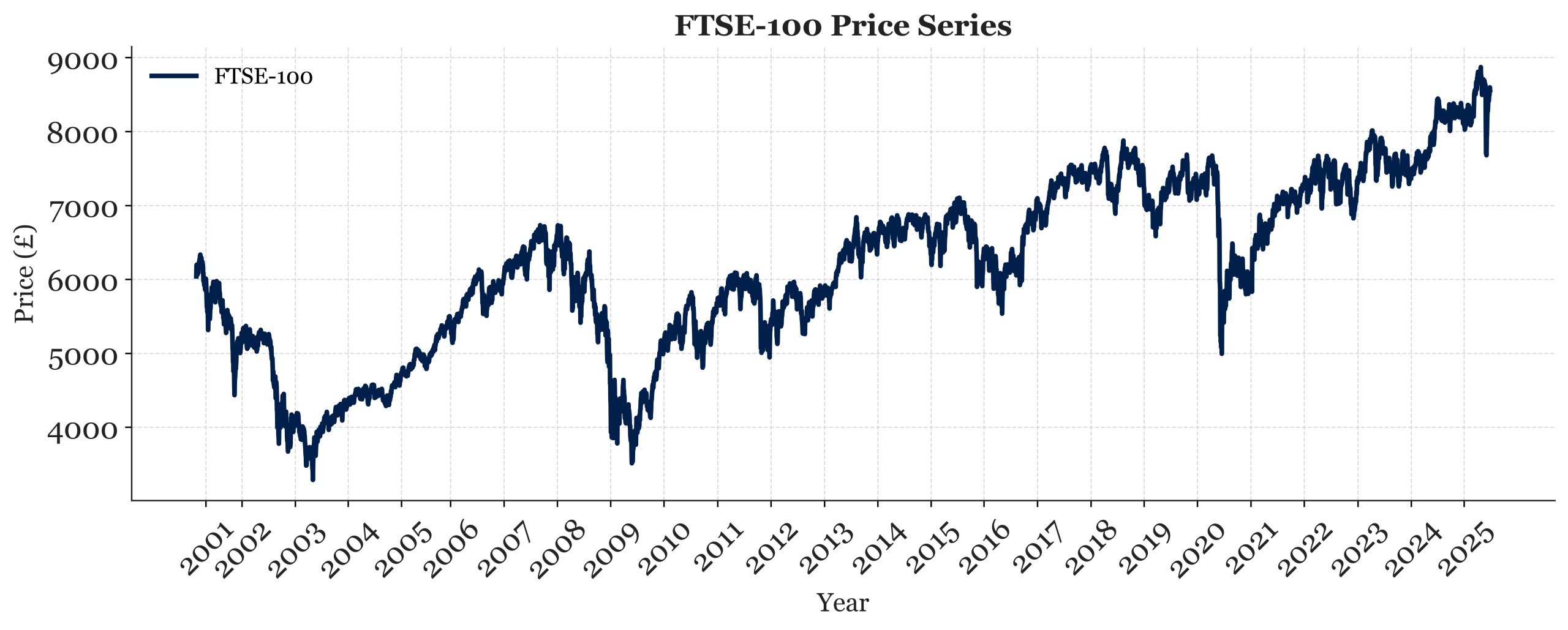
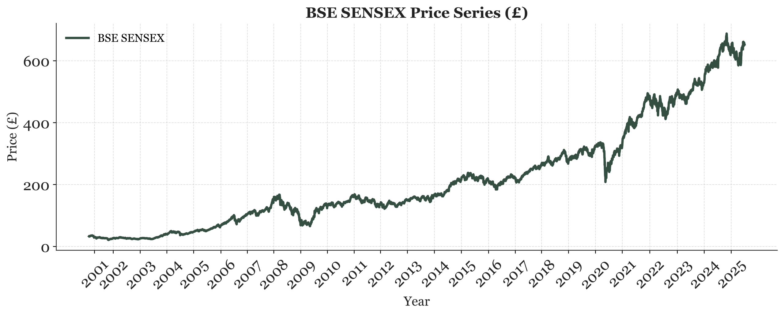
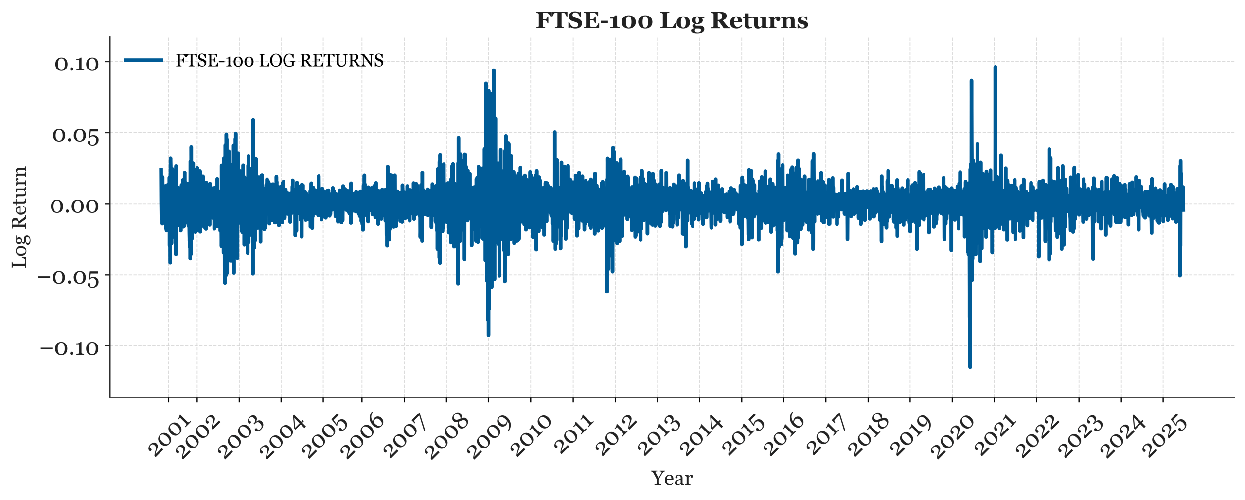
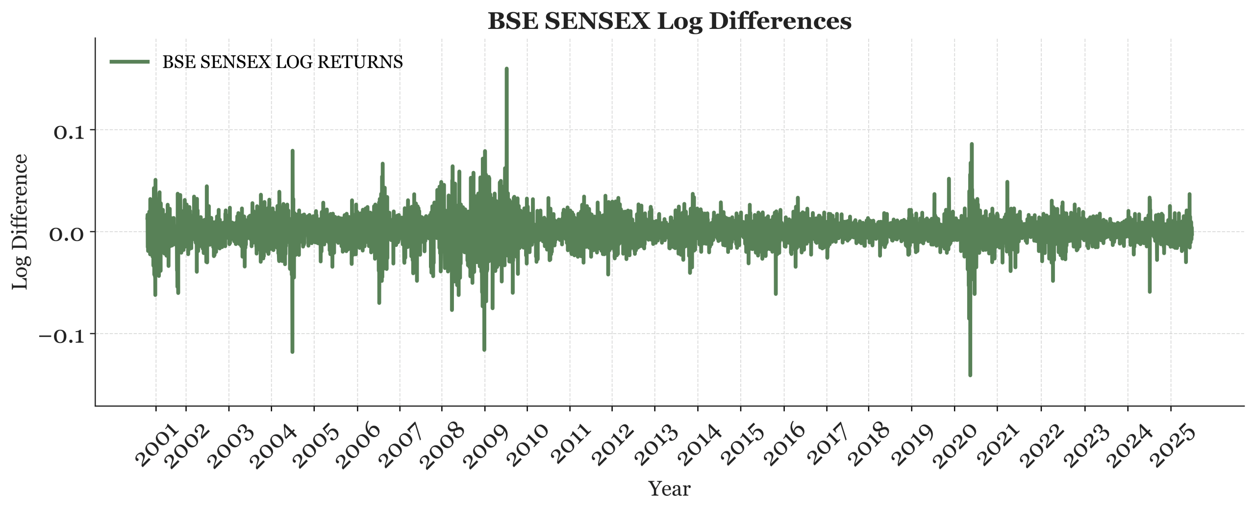
Figures 1a and 2a show the raw daily closing prices of the FTSE-100 and the BSE-SENSEX over the period 2001-2025. Both graphs depict volatile values, with changing variance throughout the sample period. Figure 1a displays a generally upward trend for the FTSE-100. Punctuated by sharp declines during the 2008 financial crisis and early 2020. Figure 2a shows the BSE-SENSEX, which exhibits a steeper upward trajectory with proportionally larger fluctuations. Figures 1b and 2b show the log differences of the daily closing prices for both stock indices. The differencing was done to make the series stationary, removing any inconsistencies or distortions in the final results for the embedding dimension, time delay and the largest LE.

Metric	FTSE-100 (UK)	BSE-SENSEX (India)
Optimal Time Delay (τ)	19	19
Optimal Embedding Dimension (m)	8	7
Estimated Lyapunov Exponent (λ)	0.1602	0.1614

Metric	FTSE (UK)	BSE-SENSEX (India)
Optimal Time Delay (τ)	19	3
Optimal Embedding Dimension (m)	10	10
Estimated Lyapunov Exponent (λ)	0.0212	0.1513

Comparative Analysis between the FTSE-100 and BSE-SENSEX

A direct comparison of the two indices reveals notable patterns. For the raw (non-stationary) price series, both the FTSE-100 and BSE-SENSEX produced similar positive LEs (0.1602 and 0.1614, respectively), with identical optimal time delays (τ = 19 for both). This similarity suggests that the raw price dynamics of both indices, which include trend and non-stationarity, exhibit comparable rates of trajectory divergence. However, once the data are log-differenced to achieve stationarity, isolating the intrinsic day-to-day dynamics from the long-term trends, a clear divergence emerges. The BSE-SENSEX’s LE (λ = 0.1513) is more than seven times that of the FTSE-100 (λ = 0.0212). The embedding parameters also differ: the FTSE-100 log differenced series has an optimal time delay of τ = 19 and embedding dimension of m = 10, while the BSE-SENSEX has τ = 3 and m = 10. The shorter optimal delay for the BSE-SENSEX suggests that its short-term dynamics contain less temporal redundancy, meaning that past price information becomes less informative more quickly, reflecting faster adjustment to new information and more reactive price behaviour. Overall, the comparison indicates that, while both markets exhibit evidence of nonlinear structure in their raw prices, the underlying stationary dynamics of the emerging market display substantially faster trajectory divergence, consistent with the expectation set out in H2.

The substantially higher estimated LE for the BSE-SENSEX log-differenced series (λ = 0.1513) compared to the FTSE-100 (λ = 0.0212) may reflect characteristics typical of emerging markets. In particular, higher retail investor participation and greater information asymmetry can give rise to herding behaviour and more speculative trading, which could generate nonlinear patterns in the price series that increase the sensitivity to initial conditions^35,36. Moreover, relatively lower liquidity in segments of the Indian market may lead to larger price impacts from individual trades. The market is also susceptible to large and volatile foreign portfolio inflows and outflows³⁷, and it has a younger regulatory infrastructure. This is consistent with the broader evidence that emerging markets tend to exhibit more informational inefficiencies and stronger nonlinear dynamics than developed markets. In contrast, the FTSE-100’s lower LE is consistent with the characteristics of a developed, more mature market, with well-established regulatory oversight by the Financial Conduct Authority (FCA), greater dominance of institutional investors, deep liquidity, and efficient information dissemination. These factors are likely to collectively dampen the nonlinear dynamics observed in the UK’s index.

However, differences in estimated LEs may also be influenced by methodological factors and noise sensitivity, so interpretations should remain cautious. The LE-based findings are best viewed as one component within the broader nonlinear analysis, and not as a standalone proof of chaos. 

Discussion

The findings of this study are broadly consistent with the literature on nonlinear dynamics in financial markets. The positive LE observed for the BSE-SENSEX log differenced series is consistent with the findings of Guhathakurta, who reported evidence of nonlinearity across both emerging and developed stock market indices¹⁷. The relatively weaker nonlinear signal in the FTSE-100 log differenced series aligns with findings by Barkoulas and Travlos¹³, who found no strong evidence of deterministic chaos in the Athens Stock Exchange, and by Gao and Wang¹⁴, who found no evidence of deterministic chaos in major futures contracts. More generally, the pattern of the LEs in both markets, with substantially stronger divergence in the emerging market, supports the conclusions of Faggini and Parziale, who suggest that financial data generally exhibit stronger evidence of nonlinearity than of definitive chaos⁷. Finally, the divergence between the raw and log-differenced series highlights the importance of preprocessing and stationarity, as emphasised by Hsieh⁶.

The time delay indicates how long it takes for the values in a time series to contain new, non-redundant information, reflecting the system’s underlying memory and dynamics. For the log-differenced series, the BSE-SENSEX showed a much shorter optimal time delay (τ = 3) than the FTSE (τ = 19), indicating that the BSE-SENSEX’s daily changes lose correlation more quickly, reflecting shorter memory and greater volatility.  An embedding dimension of m = 10 for the log-differenced series in both markets suggests that many interacting factors influence their price changes. This is consistent with the presence of high-dimensional non-linearity, which simple linear models cannot fully capture.

1/λ can sometimes be interpreted as the Lyapunov time in low-dimensional, noise-free deterministic systems, a timescale beyond which prediction becomes unreliable³⁸. However, financial markets are not noise-free, deterministic systems; stochastic factors, exogenous shocks, and structural changes influence them. Therefore, while the BSE-SENSEX’s higher LE indicates comparatively faster trajectory divergence and lower short-term predictability than the FTSE-100, the inverse values (approximately 7 days and 47 days, respectively) should be interpreted as qualitative, comparative indicators of relative divergence rates rather than literal forecast horizons.

The results of this study imply significant differences in the underlying dynamics of the UK (FTSE) and Indian (BSE) stock markets. Both markets exhibit positive LEs, consistent with nonlinear structures in their price movements, indicating that fluctuations are not solely due to exogenous random shocks but may also be partly generated internally by complex nonlinear interactions within the markets themselves³⁹. This aligns with the idea that the emergence of chaos theory in economics challenges the traditional research assumptions of stable equilibria, fully rational agents, and the preference for linear models that treat periods of great volatility as “anomalies”, all of which have historically dominated economic thought⁷.

Specifically, the FTSE’s lower largest LE and longer time delay indicate weaker nonlinear dependencies and less chaotic behaviour, suggesting that its price changes behave more like a random walk, consistent with market efficiency. In theory, a perfectly efficient market has no deterministic nature and thus zero predictability⁴⁰. However, the FTSE’s small positive (LE) indicates that a limited nonlinear structure persists in the market’s dynamics, and, given its lower rate of divergence, the series will have a longer forecast horizon than the BSE, despite being closer overall to randomness.

In contrast, the BSE exhibits a stronger nonlinear structure and more chaotic-like dynamics, as evidenced by its higher LE. This suggests a greater presence of endogenous feedback and sensitivity to initial conditions, causing price trajectories to diverge faster and limiting predictability to a shorter time frame. Although the BSE deviates further from a pure random walk, reflecting market inefficiency, this increased nonlinearity may reduce the extent to which prices can be reliably forecast. This observation is consistent with Joshi’s finding that the BSE remains inefficient in the long run and “the stocks in the index don’t absorb the price information effectively⁴¹. It means investors can identify available undervalued securities in the market and make excess returns by correctly picking them.”⁴¹

Additionally, major shocks like the 2008 Great Financial Crash and the global COVID-19 pandemic have intensified nonlinear dynamics in both markets by increasing volatility and feedback loops. In some cases, they have also caused hysteresis, leaving lasting changes that prevent a full return to pre-shock equilibrium and further give way to ongoing nonlinear behaviour.

The observed differences in nonlinear dynamics between the BSE and FTSE can be explained by their distinct market structures and levels of development. The FTSE, stemming from a developed economy, benefits from well-established regulatory frameworks, higher liquidity, and relatively efficient information dissemination, which contribute to more stable price behaviour. In contrast, the BSE, as part of an emerging market, experiences higher volatility due to several factors. While price fluctuations are a natural part of markets responding to new external information, excessive volatility in the Indian market has been exacerbated by global financial crises, large portfolio inflows and outflows³⁷, and market-specific features such as information asymmetry, lower liquidity, increased speculative trading, and the presence of retail investors.

Understanding the presence of nonlinear dynamics in the stock market and the broader economy is valuable for governments, policy-makers, and market participants. If stock market dynamics exhibit chaotic-like behaviour, then traditional linear forecasting models used by central banks and regulatory bodies may underestimate extreme risks and the potential for abrupt, nonlinear market shifts. This is especially relevant for emerging markets, where stronger nonlinear dynamics are observed, suggesting that regulators could benefit from using nonlinear tools in their monitoring and early warning systems. These findings may also enhance understanding of macroeconomic instability. According to Fernández-Díaz, chaos theory helps explain “economic instability, inflation and unemployment in an endogenous way”⁸, providing an alternative to well-established business cycle models that rely on exogenous shocks to explain the business cycle and economic instability.

Since stock market trends are commonly considered indicators of broader economic performance, governments and central banks should recognise nonlinear dynamics to better explain and manage instability across a range of economic indicators. For market participants, the presence of nonlinear dynamics highlights the limitations of standard linear approaches for forecasting and risk assessment. Incorporating nonlinear measures could improve early detection of anomalies and the effectiveness of stress-testing models. The increasing use of advanced computing, including quantum techniques, will further enhance the analysis of economic time series.

While this research offers useful perspectives, it is important to consider the study’s limitations and assumptions, which suggest areas for future research. This study primarily used the numerical methods of Takens’ embedding and the LE to detect nonlinear structure; however, the LE requires a long and cleaned time series and is also sensitive to parameter choices, which can increase the chances of error in the results due to the many factors it relies on, reducing reliability when working with noisy financial data. The method also merely indicates the presence of a nonlinear structure without identifying the underlying cause. Hence, according to Faggini and Parziale, “to produce convincing results, we have to employ all tests for chaos to exploit their different potentials and limits.”⁷ These tests should comprise numerical,  visual and geometric tools.

Moreover, Hsieh⁶ highlighted the challenge of verifying whether a process has an infinite correlation dimension with finite amounts of data, as financial economists have substantially fewer data points than other scientists. Additionally, small datasets introduce bias that may favour the detection of apparent chaos, despite its absence. These problems, along with the lack of formal statistical tests for the correlation dimension, led them to adopt alternative methods for quantifying nonlinear dynamics, such as the BDS test. They also critique the belief that financial data has no limitations, given the availability of tick-by-tick data, arguing that such data captures artificial dependencies caused by market structure, such as bid-ask bounce, and can lead to misleading tests for non-linear dynamics. To avoid this, they advised using longer sampling intervals to smooth out these effects. However, the further back one goes with the data, the more one faces the issue of non-stationarity, where changes in market conditions over time make past data less relevant. This trade-off between the need for longer data histories (to avoid artificial dependencies) and shorter histories (to avoid no stationarity) creates significant challenges in financial data analysis. The positive LEs should therefore be interpreted with caution, as finite-sample effects may lead to an overstatement of nonlinear dynamics, suggesting that these results are more indicative of nonlinear structure than definitive evidence of deterministic chaos.

A further limitation is that, although this paper compares a developing economy (India) with a developed economy (the UK), there are inherent structural and institutional differences in the markets of the two that limit the direct comparability that can be achieved. The UK’s stock market is mature, highly liquid, and dense with institutional investors, subject to strict regulations and policies. In contrast, India’s market operates under different regulatory and technological policy contexts and has lower liquidity in certain segments. These differences in investor behaviour, response to shocks and crises, and exposure to foreign capital flows can influence the detectability of nonlinear patterns, making comparisons across countries less straightforward than implied.

This study does not explicitly test for or account for structural breaks caused by major market events within the sample period, such as the 2008 global financial crisis, the European sovereign debt crisis, or the COVID-19 pandemic. Formal structural break testing, for example, using Bai-Perron tests, was not conducted. The presence of such regime-shifting events may influence the estimated Lyapunov exponents by introducing abrupt changes in volatility and market microstructure. Future research should consider breaking the analysis down into sub-periods or break-adjusted estimation to assess the stability and robustness of the findings across different market regimes. Moreover, these results cannot be generalised to other developing and developed countries without further research. As a result, direct comparisons between the two economies must be interpreted with caution and with context always considered.

It is acknowledged that relying on a single measure of nonlinear dynamics introduces limitations, and so complementary approaches would strengthen the analysis. Recurrence Quantification Analysis (RQA), for example, examines how often and how regularly a dynamical system revisits similar states in its reconstructed phase space, providing measures such as the recurrence rate and determinism that can help differentiate structured dynamics from randomness. RQA is especially useful for short and noisy data and does not require strict stationarity. Surrogate-data testing, meanwhile, compares the observed LE with those obtained from phase-randomised surrogates that preserve the linear properties of the original series, providing a formal test of whether the detected nonlinearity is significantly different from what a linear stochastic process would produce.

Another limitation of this study is that confidence intervals for the estimated LEs were not computed. Without bootstrapped standard errors or confidence bounds, the reported LE values should be interpreted as point estimates subject to uncertainty from finite sample size, choice of embedding parameters, and potential contamination from noise. Hsieh⁶ and Faggini and Parziale⁷ emphasise that small datasets can introduce bias that favours the detection of apparent chaos even when the underlying process is stochastic. Future research should incorporate resampling methods, such as bootstrapping, Monte Carlo simulation, to provide a formal quantification of uncertainty.

Conclusion

This study contributes to the growing literature on nonlinear dynamics in financial markets by providing a methodologically consistent, Lyapunov-based comparison of a developed and a developing market over 24 years.  Rather than claiming definitive proof of deterministic chaos, the findings demonstrate that both the FTSE-100 and BSE-SENSEX exhibit positive Lyapunov exponents, consistent with nonlinear or complex dynamics, with the emerging market displaying faster trajectory divergence in its stationary (log-differenced) series. These results add to the evidence from studies such as Guhathakurta¹⁷ and Fernández-Rodríguez and coworkers³³, suggesting that nonlinear structure in financial markets is a persistent feature that merits further study. The study’s expectations were largely met: both indices yielded positive LEs (consistent with H1), and the BSE-SENSEX displayed a markedly larger LE in the log differenced series (consistent with H2); however, the absence of formal statistical testing means these observations remain descriptive.

These findings are relevant for both market participants and policymakers. Nonlinear dynamics, especially in emerging markets, indicate that standard linear models may not capture the risk of extreme market movements. Incorporating nonlinear approaches into risk management and monitoring could improve the assessment of market instability. More broadly, chaos-based frameworks can complement conventional models in understanding financial price dynamics.

This study suggests several avenues for future research. First, surrogate-data testing using AAFT or IAAFT surrogates should be applied to formally differentiate deterministic chaos from stochastic nonlinearity in these price series. Second, sub-period analysis should be conducted to examine whether nonlinear dynamics intensify during external shock periods, such as the 2008 financial crisis or the COVID-19 pandemic, and whether the LE returns to pre-crisis levels afterwards. Third, the comparison should be extended to additional developed and developing markets to test to what extent these findings can be generalised. Fourth, Recurrence Quantification Analysis (RQA) should be implemented as a complementary measure to confirm the Lyapunov exponent findings. Fifth, bootstrapping or Monte Carlo methods should be applied to provide formal confidence intervals for the LE estimates. These steps, taken together, would strengthen the evidence base and address the primary limitations of this study.

References

1. Utrecht University. An Interactive guide to chaos (Chaos 101) https://chaos101.sites.uu.nl/ (n.d.). [↩]
2. T. A. P. Society. This month in physics history circa January 1961: Lorenz and the butterfly effect. https://www.aps.org/archives/publications/apsnews/200301/history.cfm (n.d.). [↩]
3. J. M. Amigó, F. Montani. Nonlinear dynamics and applications. Entropy. Vol. 27, pg. 688, 2025, https://doi.org/10.3390/e27070688. [↩]
4. Z. Sardar, I. Abrams. Introducing chaos : A Graphic Guide. Icon Books, 2004. [↩] [↩]
5. I. Klioutchnikov, M. Sigova, N. Beizerov. Chaos theory in finance. Procedia Computer Science. Vol. 119, pg. 368–375, 2017, https://doi.org/10.1016/j.procs.2017.11.196. [↩]
6. D. A. Hsieh. Chaos and nonlinear dynamics: Application to financial markets. The Journal of Finance. Vol. 46, pg. 1839–1877, 1991, https://doi.org/10.1111/j.1540-6261.1991.tb04646.x. [↩] [↩] [↩] [↩] [↩] [↩] [↩] [↩] [↩]
7. M. Faggini, A. Parziale. More than 20 years of chaos in economics. Mind & Society. Vol. 15, pg. 53–69, 2015, https://doi.org/10.1007/s11299-015-0164-1. [↩] [↩] [↩] [↩] [↩] [↩]
8. A.Fernández-Díaz. Overview and perspectives of chaos theory and its applications in economics. Mathematics. Vol. 12, pg. 92, 2023, https://doi.org/10.3390/math12010092. [↩] [↩] [↩]
9. F. Juárez. Applying the theory of chaos and a complex model of health to establish relations among financial indicators. Procedia Computer Science. Vol. 3, pg. 982–986, 2011, https://doi.org/10.1016/j.procs.2010.12.161. [↩]
10. S. C. Blank. “Chaos” in futures markets? A nonlinear dynamical analysis. Journal of Futures Markets. Vol. 11, pg. 711–728, 1991, https://doi.org/10.1002/fut.3990110606. [↩]
11. S. R. Yang, B. W. Brorsen. Nonlinear dynamics of daily futures prices: Conditional heteroskedasticity or chaos? Journal of Futures Markets. Vol. 13, pg. 175–191, 1993. [↩]
12. R. Engle. GARCH 101: The use of ARCH/GARCH models in applied econometrics. The Journal of Economic Perspectives. Vol. 15, pg. 157–168, 2001, https://doi.org/10.2307/2696523. [↩]
13. J. Barkoulas, N. Travlos. Chaos in an emerging capital market? The case of the Athens stock exchange. Applied Financial Economics. Vol. 8, pg. 231–243, 1998, https://doi.org/10.1080/096031098332998. [↩] [↩]
14. A. H. Gao, G. H. K. Wang. Modeling nonlinear dynamics of daily futures price changes. Journal of Futures Markets. Vol. 19, pg. 325–351, 1999, https://doi.org/10.1002/(SICI)1096-9934(199905)19:3<325::AID-FUT5>3.0.CO;2-6. [↩] [↩]
15. A. S. Andreou, G. Pavlides, A. Karytinos. Nonlinear time-series analysis of the Greek exchange rate market. International Journal of Bifurcation and Chaos. Vol. 10, pg. 1729–1758, 2000, https://doi.org/10.1142/s0218127400001110. [↩]
16. J. A. Scheinkman, B. LeBaron. Nonlinear dynamics and stock returns. The Journal of Business. Vol. 62, pg. 311–337, 1989. [↩] [↩]
17. K. Guhathakurta. Investigating the nonlinear dynamics of emerging and developed stock markets. Journal of Engineering Science and Technology Review. Vol. 8, pg. 65–71, 2015, https://doi.org/10.25103/jestr.081.12. [↩] [↩] [↩]
18. O. Hoffmeister. Development status as a measure of development. United Nations. 2020, https://doi.org/https://doi.org/10.18356/a29d2be8-en. [↩] [↩] [↩]
19. I. M. Fund. World economic outlook database – groups and aggregates. https://www.imf.org/en/Publications/WEO/weo-database/2023/April/groups-and-aggregates#oem 2023 (n.d.). [↩]
20. W. B. Group. World bank open data. https://data.worldbank.org/indicator/NY.GNP.PCAP.PP.CD?most_recent_value_desc=true 2024 (n.d.). [↩] [↩] [↩]
21. T. Economics. India GDP annual growth rate. https://tradingeconomics.com/india/gdp-growth-annual (n.d.). [↩]
22. N. Inamdar. India’s economy: The good, bad and ugly in six charts. BBC News. 2024. [↩]
23. P. Brien. Service industries: Economic indicators. https://commonslibrary.parliament.uk/research-briefings/sn02786/ 2025 (2025). [↩]
24. D. Gajjar. Digitalisation within and across UK infrastructure. https://post.parliament.uk/digitalisation-within-and-across-uk-infrastructure/ 2024 (2024). [↩]
25. P.-C. Hautcoeur. Why and how to measure stock market fluctuations? The early history of stock market indices, with special reference to the French case. Hal Open Science. 2006, https://doi.org/https://shs.hal.science/halshs-00590522. [↩]
26. K. Phylaktis, F. Ravazzolo. Stock prices and exchange rate dynamics. SSRN Electronic Journal. 2000, https://doi.org/10.2139/ssrn.251296. [↩]
27. D. M. Cutler, J. M. Poterba, L. H. Summers. What moves stock prices? (Spring 1989). Streetwise. pg. 56–64, 1998, https://doi.org/10.1515/9781400829408-008. [↩]
28. Investing.com. FTSE 100 historical price data – investing.com UK. https://uk.investing.com/indices/uk-100-historical-data (n.d.). [↩]
29. A. Sambo, M. Rigot, N. Meulmeester. Introduction to temporal dynamics and change. https://n-n-w-meulmeester.medium.com/a-brief-introduction-to-temporal-dynamics-and-change-b99046fd3740 (2021). [↩]
30. A. M. Fraser, H. L. Swinney. Independent coordinates for strange attractors from mutual information. Physical Review A. Vol. 33, pg. 1134–1140, 1986, https://doi.org/10.1103/physreva.33.1134. [↩]
31. M. B. Kennel, R. Brown, H. D. I. Abarbanel. Determining embedding dimension for phase-space reconstruction using a geometrical construction. Physical Review A. Vol. 45, pg. 3403–3411, 1992, https://doi.org/10.1103/physreva.45.3403. [↩]
32. T. W. F. of Exchanges. Market statistics – focus | The World Federation of Exchanges. https://focus.world-exchanges.org/issue/february-2024/market-statistics? (2024). [↩]
33. F. Fernández‐Rodríguez, S. Sosvilla‐Rivero, J. Andrada‐Félix. Testing chaotic dynamics via Lyapunov exponents. Journal of Applied Econometrics. Vol. 20, pg. 911–930, 2005, https://doi.org/10.1002/jae.805. [↩] [↩]
34. M. T. Rosenstein, J. J. Collins, C. J. de Luca. A practical method for calculating largest Lyapunov exponents from small data sets. Physica D: Nonlinear Phenomena. Vol. 65, pg. 117–134, 1993, https://doi.org/10.1016/0167-2789(93)90009-p. [↩]
35. E. C. Chang, J. W. Cheng, A. Khorana. An examination of herd behavior in equity markets: an international perspective. Journal of Banking & Finance. Vol. 24, pg. 1651–1679, 2000, https://doi.org/10.1016/s0378-4266(99)00096-5. [↩]
36. S. Bikhchandani, S. Sharma. Herd behavior in financial markets. IMF Staff Papers. Vol. 47, pg. 279–310, 2000, https://doi.org/10.2307/3867650. [↩]
37. H. Goudarzi, C. S. Ramanarayanan. Modelling and estimation of volatility in the Indian stock markets. International Journal of Business and Management. Vol. 5, 2010, https://doi.org/10.5539/ijbm.v5n2p85. [↩] [↩]
38. P. M. Cincotta, C. M. Giordano, I. I. Shevchenko. Revisiting the relation between the Lyapunov time and the instability time. Physica D: Nonlinear Phenomena. Vol. 430, pg. 133101, 2022, https://doi.org/10.1016/j.physd.2021.133101. [↩]
39. C. G. Gilmore. Detecting linear and nonlinear dependence in stock returns: New methods derived from chaos theory. Journal of Business Finance &amp Accounting. Vol. 23, pg. 1357–1377, 1996, https://doi.org/10.1111/1468-5957.00084. [↩]
40. E. F. Fama. Random walks in stock market prices. Financial Analysts Journal. Vol. 51, pg. 75–80, 1995, https://doi.org/10.2469/faj.v51.n1.1861. [↩]
41. Dr. D. Joshi. Testing market efficiency of the Indian stock market. SSRN Electronic Journal. Vol. 2, 2012, https://doi.org/10.2139/ssrn.3307352. [↩] [↩]