
Abstract
As technology has increased, energy demand has also increased. Conventional methods of producing energy also produce harmful byproducts that damage the environment. Due to this issue, people have turned to renewable energy sources like solar power as an alternative. However, few consider the environmental impact of these solar panels. Most studies evaluate the production and economic potential of solar panel sites rather than their ecological effects. This study attempts to address this problem by developing a convolutional neural network (CNN) to assess the environmental suitability of solar panel locations. This paper is an observational and cross-sectional study that focuses on the Midwest United States. After preprocessing the three-channel input, the model consists of 3 convolutional blocks, each with 2 convolutional layers. The model is then trained and tested to ensure accuracy. Results-wise, evaluation metrics like accuracy, recall, and precision ranged from ~0.95 to ~0.99. This demonstrates that the CNN can successfully reproduce a heuristic ecological suitability framework derived from environmental layers. However, since the labels are not independent ecological evidence, the model should be interpreted as a rule-distillation framework rather than validated ecological suitability. Additionally, future research can add temporal data or baseline models to improve the CNN.
Keywords: Convolutional Neural Network, Environmental Suitability, Midwest, Solar Panels, Ecological Effect, Key Wildlife Areas, Critical Habitats, Energy
Introduction
According to the U.S Energy Information Administration (EIA), in 2024, electric power generation released 1,427 million metric tons of carbon dioxide1. Carbon dioxide is a compound that may not be toxic to humans, but it is a major contributor to global warming. For this reason, many countries have begun to seek out more renewable energy sources to prevent irreparable environmental damage. According to the International Energy Agency (IEA), solar power is expected to expand significantly within the next five years2. As solar PV cells become more prevalent, it is important to evaluate their possible implications carefully. While a more reliable and widespread renewable energy source can lead to vast improvements to the environment through the reduction of emissions, there may also be negative environmental consequences. To evaluate and minimize these consequences, spatial machine learning can be implemented. However, current solar site selection models mainly focus on energy production and economics rather than ecological impacts.
Changes to the natural ecosystem can cause unseen ripple effects to the nearby flora and fauna. Solar PV installation, specifically that of the utility-level scale, requires extensive stretches of land. This can cause habitat fragmentation and soil disturbance. Additionally, these installations can disturb natural wildlife. For example, solar farms have reflective surfaces. These surfaces can act as an illusion of water, altering animal behavior3. While this alteration isn’t inherently harmful, it can cause a chain reaction of disturbances to migration and other vital animal habits. Furthermore, such facilities can increase the risk of flying creature collisions and burn injuries3. Therefore, it is paramount to evaluate the location of panel installations to ensure that the environmental disturbance will be minimal.
As mentioned before, a possible approach to assessing these locations is the use of spatial machine learning. Spatial machine learning is the use of ML algorithms on data that has a spatial aspect. If comprehensive data is fed into these models, they can become an automated process to determine the least environmentally impactful locations of PV cells.
Environmental factors for the model to consider in solar PV sites are critical habitats, key wildlife areas, and cultivated land. Critical habitats are imperative to keep in consideration as changes to the ecosystem could become devastating for at-risk species. Key wildlife areas should be avoided to cause the least disruption in breeding and migration cycles. Finally, solar panels that are installed in cultivated land can have a smaller impact on the environment as the area is already heavily altered. This model focuses primarily on the Midwest of the United States, as there is potential for solar expansion, high biodiversity and ecosystem diversity, and comprehensive, accessible geospatial data of the area.
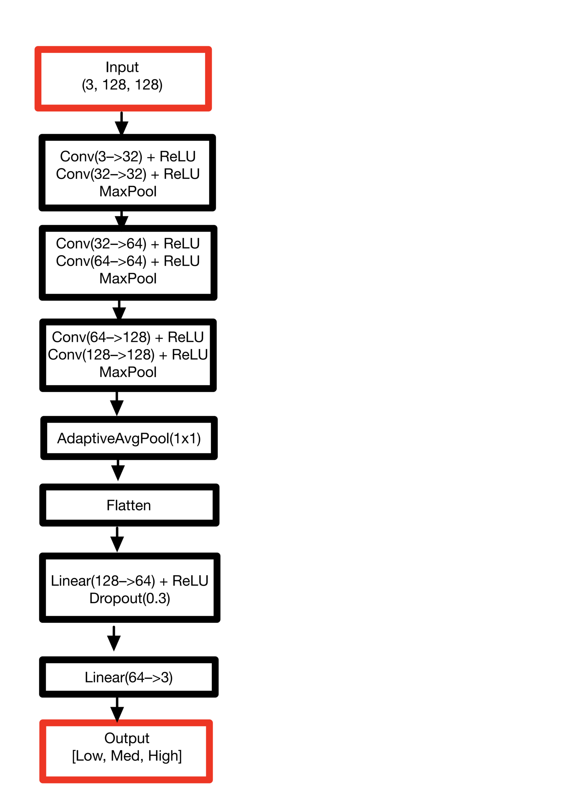
This model differs from current solar panel-focused models as it is centered on the environmental impact rather than predicting energy or economic viability. Additionally, this model incorporates spatial cross-validation to ensure accurate results. This model does contain a few limitations. First of all, the model is being trained on one specific area, making the global generalization uncertain. Furthermore, there is no baseline model to compare with, so efficiency in this specific structure is not determined. Moreover, temporal data is not included, and therefore, seasonal and daily changes to climate are not considered. Finally, the model does not use independently verified ecological suitability labels for the evaluative formula, making the framework more of a rule-distillation type than creating a validated ecological suitability model. This means the model is trained to reproduce a rule-based framework rather than directly predict environmental outcomes. This model was designed to be a CNN with an architecture as seen in Figure 3. After preprocessing, tile generation, labeling, and training, locations are evaluated. Future applications of this model consist of being used as a pre-screening tool for locations or incorporated into upcoming models. The use of this model ensures that ecological impacts are evaluated before any panel is installed.
In conclusion, the research question for this paper is: Can a multi-channel CNN classify environmentally suitable solar sites using ecological data? And as mentioned before, this study was able to design a CNN model to accurately evaluate locations.
Literature Review
Traditional geographic information system (GIS) based solar site selection typically incorporates spatial analysis such as Multi-Criteria Decision Making (MCDM) and weighted overlay, to decide on optimal solar panel farm locations. GIS allows for the layering of multiple factors to support decision-making and has recently increased in popularity.
For instance, Gigović et al.’s study created a hybrid GIS-MCDA-MABAC model to discover the most optimal locations for wind farms based on 11 selection criteria4. His research resulted in the discovery of 321 square kilometers of suitable land for wind power. Similarly, Anwarzai and Nagasaka’s research used a GIS-MCDA approach to determine the potential for wind and solar energy within Afghanistan by considering available technology and site conditions, calculated an annual potential generation of 140,982 GWh from solar PV cells and 342,521 GWh from wind power5. Both studies incorporated a similar architecture to determine optimality and energy generation. Yang initiated a study in China to determine the potential for large-scale solar power generation using a GIS-based model6. Likewise, Zhang used ArcGIS technology to predict that Xinjiang Province would be the ideal location for a large-scale photovoltaic site7.
In South-Central Vietnam, Nguyen’s research created a GIS-based simulation to identify the optimal site for a solar farm within South-Central Vietnam8. His study used eight criteria to decide location: solar radiation, land surface temperature, distance to substation, main road, land use, slope, residential area, and historical/tourist sites.
In contrast to site-selection, Pojados and Abundo’s study created a four-stage spatial energy model using GIS and Cost-Benefit Analysis (CBA) to evaluate the suitability of renewable energy9. The framework initially identifies suitable locations but eventually focuses on assessing the economic viability of renewable energy.
Although some of the aforementioned studies do incorporate a form of ecological factors within the criteria, the focus of such models remains predominantly on discovering and evaluating locations for power production and economic viability. For example, while Yang included some environmental considerations in calculating the potential carbon footprint reduction through this project, he does not consider the installation’s impact6. Similarly, Zhang’s study lacked consideration of the environmental effects, with the main consideration being solar energy potential7. And while Nguyen’s model seems comprehensive in that it considers the factors that determine power output (solar radiation, temperature, slope, etc) and its effect on communities nearby (historical/tourist locations, residential area, distance to main road and substation, etc), he doesn’t incorporate ecological spatial layers, meaning environmental consideration is conspicuously absent8. Existing models seem to mainly prioritize energy output and economic viability rather than environmental protection.
However, the ecological effect should be considered, as there can be major environmental impacts with the installation of renewable energy. Solar energy facilities require a massive amount of land use, and in areas of high biodensity, this can become problematic10. Additionally, the land required for the infrastructure to support such panels can be around “2.5 times the area of the panels themselves”11. According to Gasparatos, the major habitat change that can occur through installation and preparation is habitat fragmentation, which becomes prevalent, leading to an impediment to species movements, which consequently affects predator-prey relationships, food availability, and hiding places for wildlife11. Harmful effects are seen in bat species as well. Results from a study by Barre indicate that “implementation of solar farms results in a reduction of habitat quality for bats”12. Additionally, evidence has been presented that solar parks can “alter soil prokaryotic and fungal diversity” due to changes in soil water content13. In fact, PV panels can lead to a “decrease in network stability and an increase in vulnerability” for soil bacteria14. This change in microclimate was made evident in another study by Li, finding that “light intensity, wind flow, and soil temperature were significantly reduced” in certain areas15. When analyzing vegetation indices at points near solar panels, it was found that “solar panels had a negative impact on the vegetation”16. This could be in part due to the fact that the environmental changes that occur due to PV construction put pressure on seed germination17. Effects on plant life can differ based on ecosystem type. In deserts, panels result in an “increase in vegetation biomass and a decrease in vegetation diversity”18. It was also discovered that “shading from solar panels altered the abundance and timing of floral blooms visited by pollinators”19. While this change is not necessarily negative, it does impact the ecosystem. There are also more direct negative effects. According to Valera, birds are the “main casualties” of photovoltaic plants due to reasons such as overlap in critical habitat20. In fact, studies have found that after installation “Simpson diversity and Pielou evenness decreases”21. These negative effects are further reinforced by a study in the western rangelands. The study found that solar expansion caused “habitat loss” and “introduced barrier effects” to resident species22. Furthermore, a study on projected solar growth in the United States found a“substantial overlap of projected solar energy development with high-value land for animal movement”23. Solar power production effects aren’t just limited to land. A study on water ecosystems states that “primary production of benthic microalgae in PV is likely inhibited”24. In addition, water quality parameters in photovoltaic zones “all exhibited a decrease compared to non-photovoltaic zones”25. Moreover, the act of building solar power facilities “releases CO2 as a result of vegetation clearing”26. Current models must incorporate ecological factors into their decision-making for solar site selection to prevent detrimental effects
Specifically, this study uses a multi-channel convolutional neural network (CNN). In a study by Akar, a 3D CNN was found to outperform other machine learning algorithms in the classification of spatial distribution, with “an 11% advantage” compared to other versions27. Moreover, Austin-Gabriel et al. found “enhance[d] classification” of power plant energy estimations by pipelining GIS features into a developed CNN and Vision Transformer28. Jeong and Kim’s study proposed a space-time convolutional neural network (CNN) to predict photovoltaic cell generation within California, New York, and Alabama29. Their results indicate that this method improves accurate forecasting by 33% and reduces error by up to 40%. Similarly, in a study by Vlaminck, experiments using his developed CNN had a success rate of over 90% in classifying and detecting PV defects30. Since the model made in this study depends predominantly on similar visual and spatial data, a CNN is a suitable choice for the framework. The CNN created is multi-channel to incorporate a holistic amount of factors for site evaluation. However, this CNN is just a step towards spatial modeling as it still depends on a set formula and weights.
This paper addresses the gap in the literature, which is the lack of consideration of the ecological effects of solar installation. Moreover, this study creates a novel site classification model using a deep learning architecture to transition the focus from primarily economic or productivity to environmental. With the validation of this paper, sections of the created model can be incorporated into other frameworks to ensure that environmental consequences can be evaluated efficiently without being overlooked. Additionally, the logic behind the algorithm can be reflected within other areas of the world to create much of the same effect.
Methods
The study is overall an observational and cross-sectional study. The area analyzed includes the Midwest United States. This section was chosen for its high potential in solar power. The area also has a high ecosystem diversity and comprehensive available data, making it preferable. The independent variables in this study are critical habitats, key wildlife areas, and cultivated land. The dependent variable is the suitability class.
Data Sources
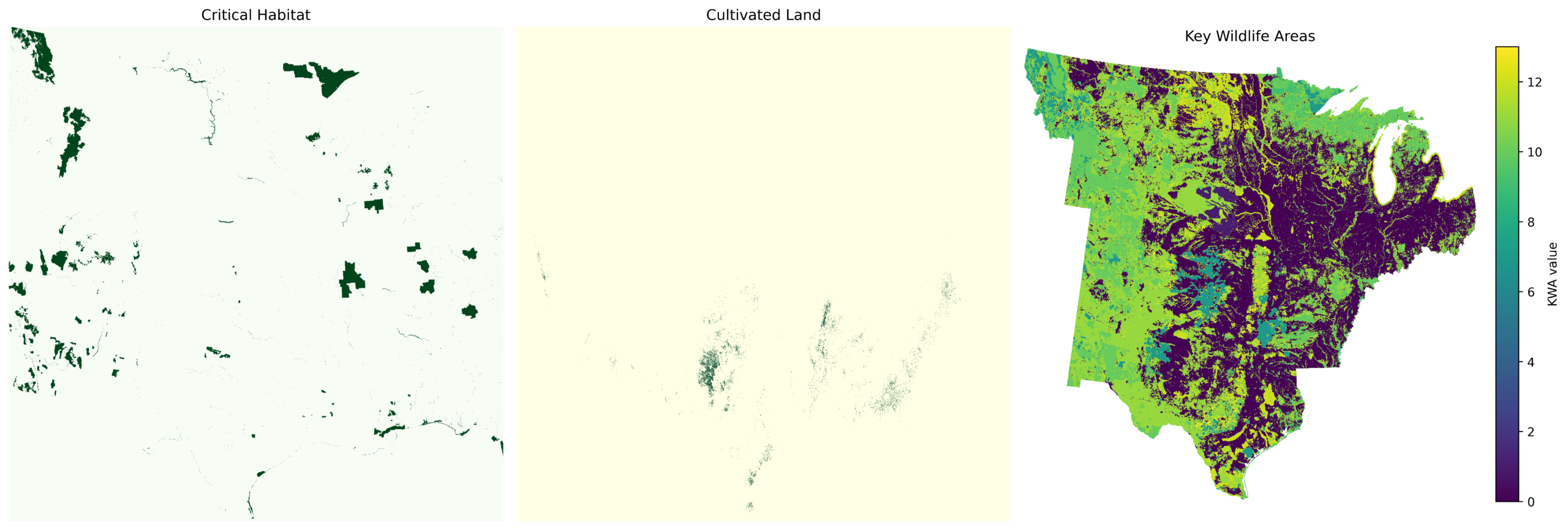
The coordinate system used is that of the KWA raster, where habitat polygons and CDLS (cultivated land from the Cropland Data Layer) tiles were reprojected to match the KWA CRS. This means that the exact Midwest boundary in which the model acts on is the boundary of the KWA dataset. This ensures there is no spatial distortion and the pixels are properly aligned. It also ensures that there is consistent tile extraction from each dataset. The data for the Key Wildlife Areas was sourced from The Nature Conservancy, the data for the cultivated land was sourced from the USDA National Agricultural Statistics Service, and the data for the critical habitats was sourced from the U.S Fish and Wildlife Service. The areas included in the KWA are whooping crane stopover sites, threatened/endangered species, water/wetlands, protected/managed lands, intact natural habitats, climate-resilient lands, and areas of other unspecified biodiversity significance.
The data types of the KWA and CDLS datasets are rasters, where critical habitat is a vector. Therefore, the final CNN input is a three-channel raster tile with the first channel being the habitat mask, the second being the cultivated land mask, and the third being the normalized KWA.
Preprocessing
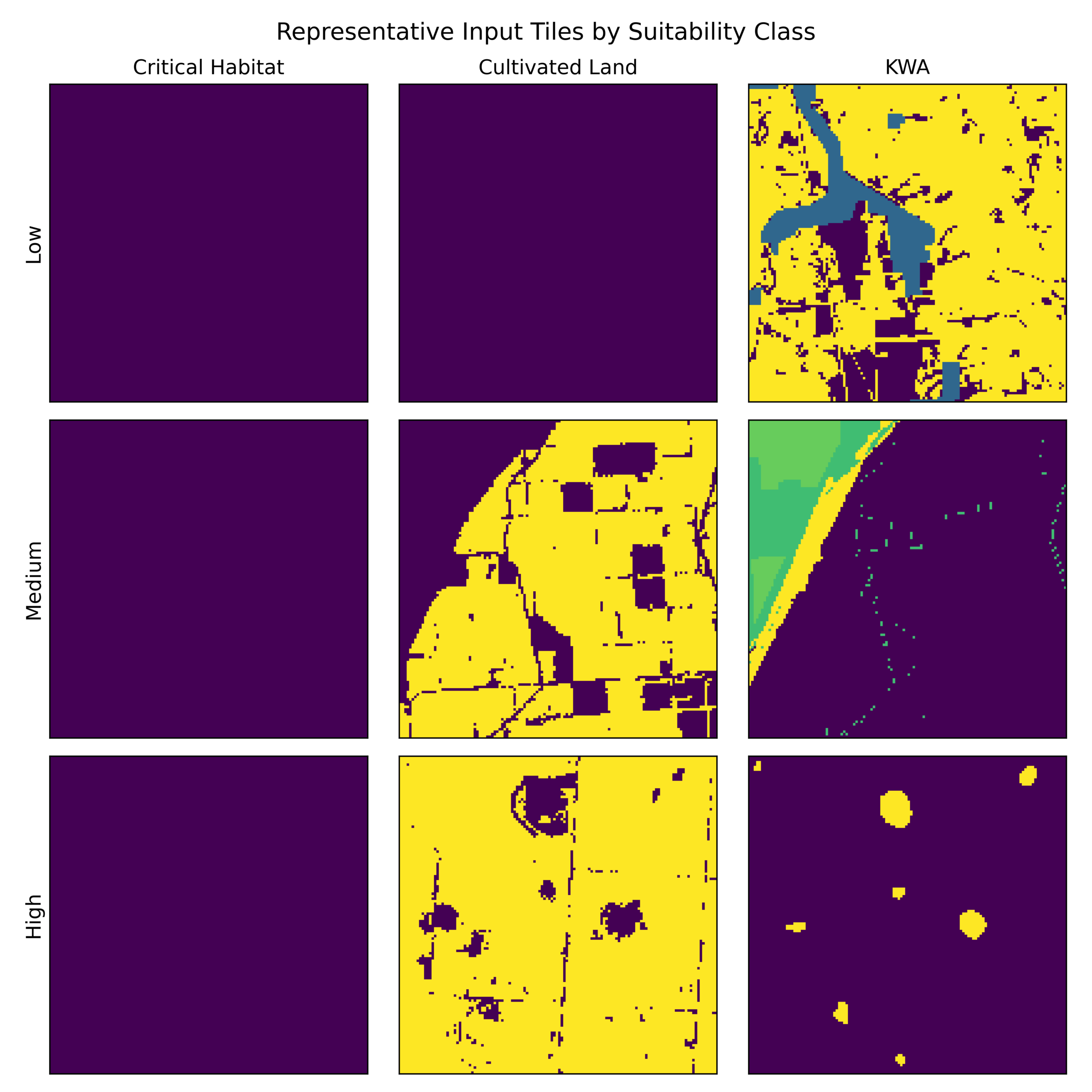
For preprocessing, the habitat layer was reprojected to match the KWA CRS and was rasterized per tile using a spatial index. The CDLS was converted to a binary cultivated mask, with it being resampled to tile size using the nearest neighbor. For the KWA, nodata was replaced with zero, and it was normalized using the estimated global maximum value. Each tile is a three-channel image containing the habitat, cultivated land, and KWA data as shown in Figure 1. Tiles containing minimal data were removed to prevent learning from empty regions. A tile was considered empty if the KWA mean was less than 0.01, the habitat fraction was zero, and the cultivated land fraction was zero.
| Dataset | Source | Access Date | Year | Resolution | CRS | NoData | Processing |
| KeyWildlifeAreas Solar GeoTIFF | TNC Site Renewables Right | Jan 2026 | N/A | 30 m | ESRI:102039 | <0.01 →0 | Master layer; nearest-neighbor resampling to 128×128; normalized to [0,1] |
| USDA Cropland Data Layer (CDL) | USDA NASS CDL | Jan 2026 | 2024 | 30 m | EPSG:5070 | → 0 | Cropped to KWA; nearest-neighbor resampling to 128×128; binary mask |
| USFWS Critical Habitat Polygons | U.S. Fish & Wildlife Service | Jan 2026 | N/A | Vector | EPSG:4326 | N/A | Reprojected to KWA; rasterized to aligned 128×128 grid |
Tile Generation
The final raster resolution was 30m, and each tile size was 128 x 128 pixels. Spatially, each tile was 3.84 km x 3.84 km. Therefore, the raster dimensions of each tile are (3, 128, 128), where each tile is stored as a float32.
The number of tiles used is 2000, where sampling was used on a quota basis: 500 each for habitat heavy, high KWA, cultivated land, and background. A tile is considered habitat heavy if more than 10% is critical habitat. The tile is considered high KWA if there is high wildlife importance, and it is considered cultivated if agricultural land is the most dominant. Finally, a tile is considered background if the data is neutral or mixed. As the number of tiles was based on quotas, the type of sampling used was stratified sampling to ensure class diversity and to prevent any imbalance.
Labeling Strategy
The environmental score is calculated through the formula: score = 1- (0.6*KWA+0.3*habitat-0.1*cultivated). The formula can be further simplified into the form score = 1 – 0.6*KWA – 0.3*habitat + 0.1*cultivated. Since KWA has the strongest ecological importance as it conveys overall wildlife behavior and sensitivity, it was assigned the largest weight. Critical habitats have a high conservation importance and therefore reduce suitability, but as habitats are more localized compared to KWA, KWA has double the weight (0.6). Habitat is assigned a weight of 0.3 as it is less harmful than KWA. The lowest score should be above zero to prevent absolutes. Finally, since cultivated land is land that has already been altered, it increases suitability as it reduces the area of change. Therefore, it increases the score. However, this increase in ecological suitability has not been substantially quantified and therefore has the lowest weight. Nevertheless, these weights are based on reasoning rather than empirical validation. The higher the score is, the more suitable the location is for development based on the heuristic formula. The bottom third of scores is classified as low suitability, the middle third as medium suitability, and the highest third is classified as high suitability. If KWA and habitat are zero while cultivated is 1, the score will be 1.1. This will likely classify the tile as highly suitable. However, if the habitat fraction is greater than 10%, the location is forced into low suitability. This is implemented to enforce conservation priority. The final distribution is approximately balanced, with the low classification having more because of the habitat override. The three-classification format avoids oversimplification in binary classification. It also stabilizes the CNN training, while allowing for interpretation in outside circumstances. However, it is important to keep in mind that the category thresholds are statistical and not ecologically validated; therefore, the score doesn’t necessarily determine how environmentally safe locations are.
Model Architecture
This network contains 3 convolutional blocks with 2 convolutional layers per block, as seen below in Figure 3. The three-channel input allows the CNN to learn the spatial interactions between environmental factors, such as where they overlap and influence each other.
After each block, there is max pooling and then finally global average pooling. The first block extracts the lower-level spatial features like boundaries and patch shapes. The output shape is (32, 64, 64). The second block doubles the depth of the features and learns spatial patterns of a middle level: patch density, clusters, etc. The output shape is (64, 32, 32). The third block captures higher-level spatial structure. It learns feature dominance, landscape composition, and the texture of environmental patterns. The output shape is (128, 16, 16). Finally, the global average pooling reduces this shape to (128, 1, 1) before flattening it into (128). Global average pooling was chosen as it conveys how strong each feature is in a tile rather than where the feature is, which suits the purpose of this model better. Furthermore, global average pooling prevents overfitting and partially implements spatially global reasoning as indicated in Table 7 for the ablation test results. The tiles are 128×128 to balance spatial context with computational efficiency. Since it is at 30m resolution, each tile has an area of 3.84 km x 3.84 km. This is large enough to capture the most important patterns while being small enough for training and processing to be efficient. The final CNN contains ~295,459 parameters. This count is large in comparison to the dataset, so the model is regularized using methods like dropout, weight decay, early stopping, and spatial cross-validation.
| Component | Value | Component | Value |
| Input Shape | 3 × 128 × 128 | Output Classes | 3 (Low, Medium, High) |
| Conv Blocks | 3 | Filters | 32 → 64 → 128 |
| Kernel Size | 3 × 3 | Stride | 1 |
| Padding | 1 | Pooling | MaxPool 2 × 2 |
| Global Avg Pooling | Yes | Dense Layers | 128 → 64 → 3 |
| Activation | ReLU | Dropout | 0.30 |
| Total Parameters | 295,459 | Trainable Parameters | 295,459 |
| Framework | PyTorch 2.9.1+cpu | Hardware | CPU |
| Random Seed | 42 | Repeated Runs | 1 |
| Metrics Averaged Across Runs | No | Loss Function | Cross-Entropy |
| Optimizer | Adam | Initial Learning Rate | 0.01 |
| Scheduler | ReduceLROnPlateau | Scheduler Factor | 0.5 |
| Scheduler Patience | 3 epochs | Weight Decay | 1×10⁻⁴ |
| Gradient Clipping | 1.0 | Batch Size | 64 |
| Maximum Epochs | 50 | Early Stopping Patience | 8 epochs |
Training Setup
The hardware used for training was the CPU, and the learning rate was set to be 1e-3. The loss function incorporated into this model is Cross-Entropy Loss, as it is what is typically used for multi-class classification models such as this one. Since the classes of this model (Low, Medium, High) are mutually exclusive and categorical, Cross-Entropy Loss fits ideally as a loss function. The optimizer used is AdamW, as it has adaptive learning rates and better generalization compared to Adam. The activation function used is ReLU to introduce non-linearity. In early layers, the activation function emphasized the transitions and edges of regions. In the middle layers, ReLU allows feature interactions and nonlinear combinations of local patterns. Finally, in the deeper layers, ReLU encourages nonlinear ecological gradients. The pooling layer incorporated into this model is MaxPool2d, which is used after each convolutional block, as shown in Figure 3. After the final pooling, a global average pooling is applied. This reduces the number of features to 128 to prevent overfitting and force global reasoning.
Within this model, if validation loss no longer improves, the learning rate will be halved. Since environmental data can have small oscillations, learning rate reduction can allow for a more stable convergence and better fine-tuning in later epochs. Additionally, this model incorporates early stopping such that if the validation loss doesn’t improve in eight epochs, the training will stop. This prevents memorization and wasted computational power. Moreover, the included gradient clipping prevents training instability and exploding gradients. There is a batch size of 64 to allow for stable gradient estimates while maintaining reasonable training times. There are 50 epochs; however, most folds stop earlier due to the early stopping feature. The regularization techniques used are the dropout, weight decay, early stopping, spatial CV, and GAP features. These features prevent overfitting and improve generalization. They also provide spatial variability in the dataset.
Cross-Validation Strategy
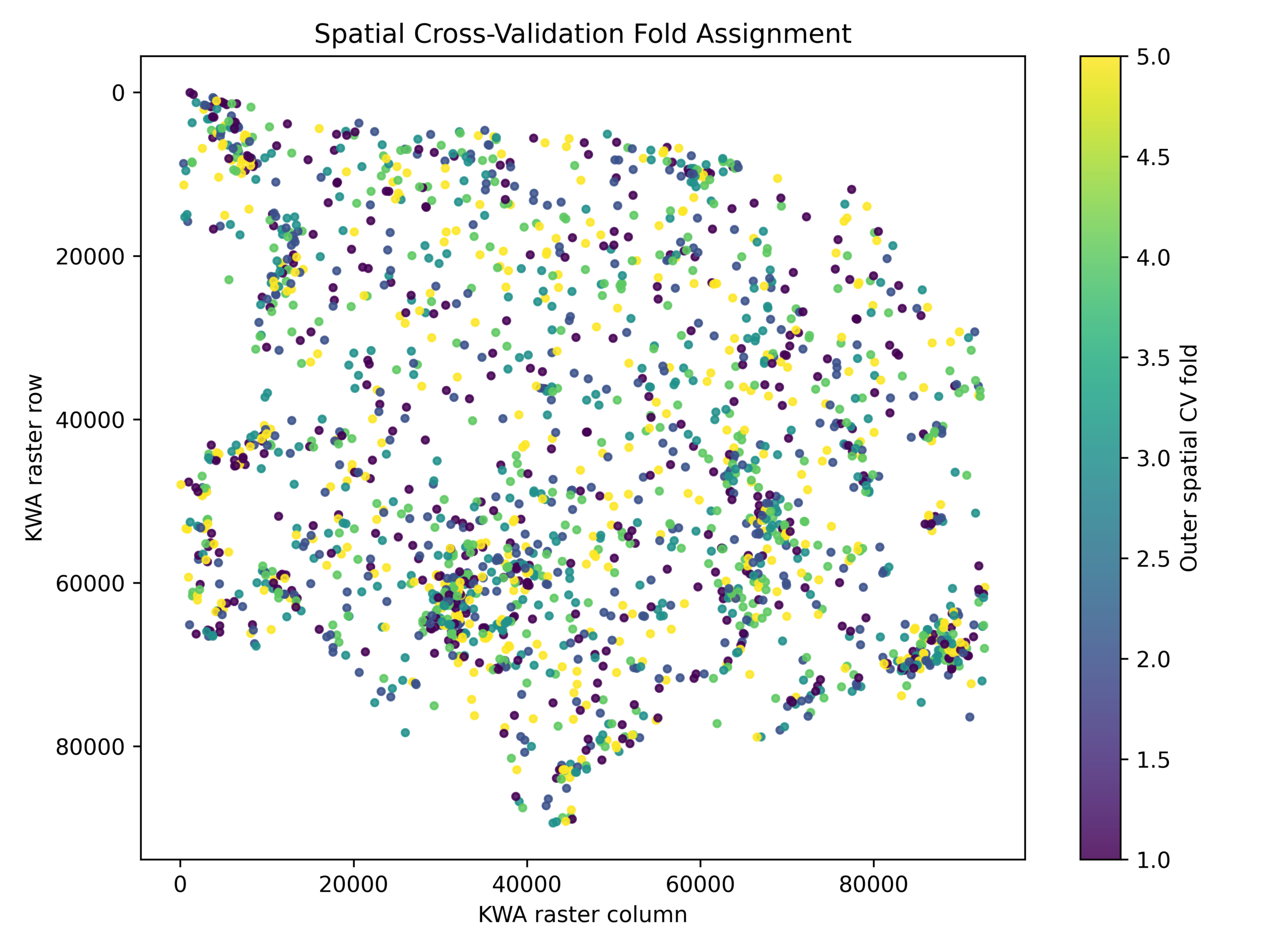
This model includes a five-fold cross-validation. The outer loop contains five spatial folds, while the inner loop uses a five-fold spatial split for validation. For each outer fold, around 70% of the data is used for training, 20% of the data is used for validation, and about 10% are used for testing. The reason for spatial CV is that it prevents overly optimistic accuracy or memorization of geography. Furthermore, it prevents spatial leakage. This means the cross-validation stops nearby tiles from appearing in both the testing and training data.
Tiles are assigned to blocks before cross validation. Group identifiers were created using the formula group = (row//512) x 1000 + (col//512) where each tile belongs to a unique 512×512 pixel block. Each spatial block represents about 15.36 km x 15.36 km. Tiles belonging to the same spatial block can’t appear in both training and testing sets.
The evaluation metrics that are considered are accuracy, macro F1, balanced accuracy, per-class recall, Moran’s I, and confusion matrices. The accuracy conveys overall correctness. Macro F1 treated each class equally, while penalizing poor minority-class performance. Balanced accuracy makes sure to account for class imbalance. Per-class recall is important to consider, as missing low suitability areas can be harmful, and missing high suitability areas reduces efficiency in planning. The confusion matrix conveys where the model confuses different classifications based on the reproduction of the given formula. Balanced metrics are important as it prevents a misleading high accuracy rate.
| Fold | Train | Val | Test | Min Dist (km) | Mean Dist (km) | Moran’s I | p-value |
| 1 | 1286 | 312 | 402 | 1.32 | 27.29 | -0.020 | 0.273 |
| 2 | 1289 | 313 | 398 | 2.86 | 27.86 | -0.014 | 0.471 |
| 3 | 1286 | 328 | 386 | 1.32 | 28.43 | 0.026 | 0.141 |
| 4 | 1267 | 329 | 404 | 2.21 | 24.76 | 0.029 | 0.068 |
| 5 | 1275 | 315 | 410 | 2.03 | 27.43 | -0.008 | 0.467 |
Final Code→https://github.com/AriaMitra/EnvironmentalSuitabilityofSolarInstallations/tree/main
Results
The model includes 5-fold spatial cross-validation as mentioned earlier. This approach prevents spatial leakage and enables realistic generalization. As seen in Table 3, the minimum distance between a test tile and the nearest training tile ranges from 1.32 km to 2.86 km, while the mean distance ranges from 24.76 km to 28.43 km. Moran’s I was calculated on binary prediction residuals to see whether prediction errors remained spatially clustered. Since the values remained close to zero (-0.020 to 0.029) and the p-values all exceeded 0.05, there is evidence that the spatial cross-validation reduced geographic leakage. The overall results, as seen in Table 4, ended with accuracy having a mean of 0.9796 and a standard deviation of 0.0108, macro f1 having a mean of 0.9759 and a standard deviation of 0.0125, balanced accuracy having a mean of 0.9759 and a standard deviation of 0.0104, low recall having a mean of 0.9869 and a standard deviation of 0.0226, medium recall having a mean of 0.9515 and a standard deviation of 0.0214, high recall having a mean of 0.9894 and a standard deviation of 0.0117, low precision having a mean of 0.9886 and a standard deviation of 0.0068, medium precision having a mean of 0.9580 and a standard deviation of 0.0420, and high precision having a mean of 0.9820 and a standard deviation of 0.0176. Almost every fold had an accuracy between 96% and 99%, with a minimal standard deviation. Additionally, the number of tiles that were reassigned due to habitat override is 500.
| Accuracy | 0.9796 ± 0.0108 |
| Macro F1 | 0.9759 ± 0.0125 |
| Balanced Accuracy | 0.9759 ± 0.0104 |
| Recall_Low | 0.9869 ± 0.0226 |
| Recall_Medium | 0.9515 ± 0.0214 |
| Recall_High | 0.9894 ± 0.0117 |
| Precision_Low | 0.9886 ± 0.0068 |
| Precision_Medium | 0.9580 ± 0.0420 |
| Precision-High | 0.9820 ± 0.0176 |
A sensitivity analysis was also included to map the changes in class labels if the variable weights were slightly altered. As seen in Table 5, in the case where KWA is given a weight of 0.5, critical habitat is given a weight of 0.4, and cultivated land is given a weight of -0.1, the percentage of tiles that change classification is 5.30%. When KWA is given a weight of 0.7, critical habitat is given a weight of 0.2, and cultivated land is given a weight of -0.1, the percentage of tiles that change classification is 1.20%. When KWA is given a weight of 0.6, critical habitat is given a weight of 0.3, and cultivated land is given a weight of -0.2, the percentage of tiles that change classification is 1.70%. Finally, when KWA is given a weight of 0.6, critical habitat is given a weight of 0.3, and cultivated land is given a weight of -0.05, the percentage of tiles that change classification is 1.60%.
| More habitat (0.5 / 0.4 / -0.1) | 5.30% |
| More KWA (0.7 / 0.2 / -0.1) | 1.20% |
| More cultivated (0.6 / 0.3 / -0.2) | 1.70% |
| Less cultivated (0.6 / 0.3 / -0.05) | 1.60% |
The training curves in Figure 5 illustrate that in early phases/epochs, there is a rapid drop in training and validation loss, while accuracy jumps to the ~90% range. In the middle phase, there are more gradual improvements with the validation accuracy often reaching almost ~97%. In the late phase, there are some spikes.
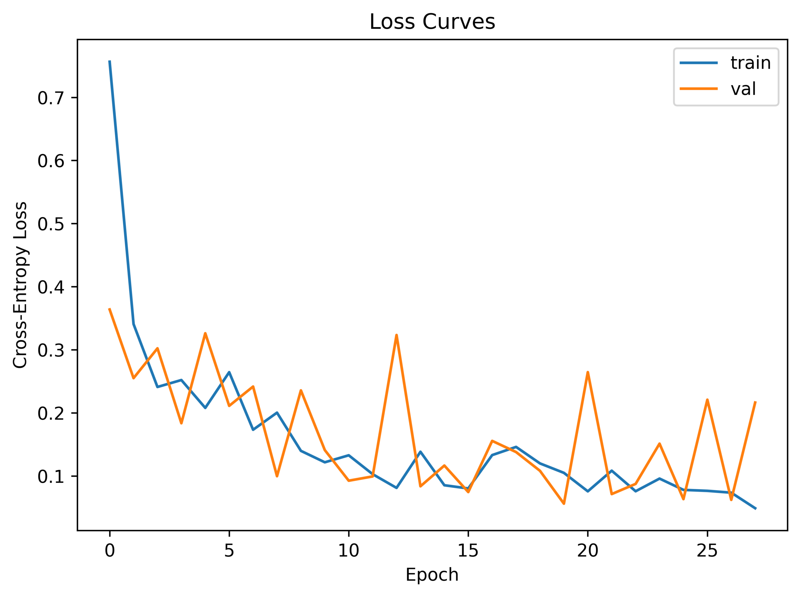
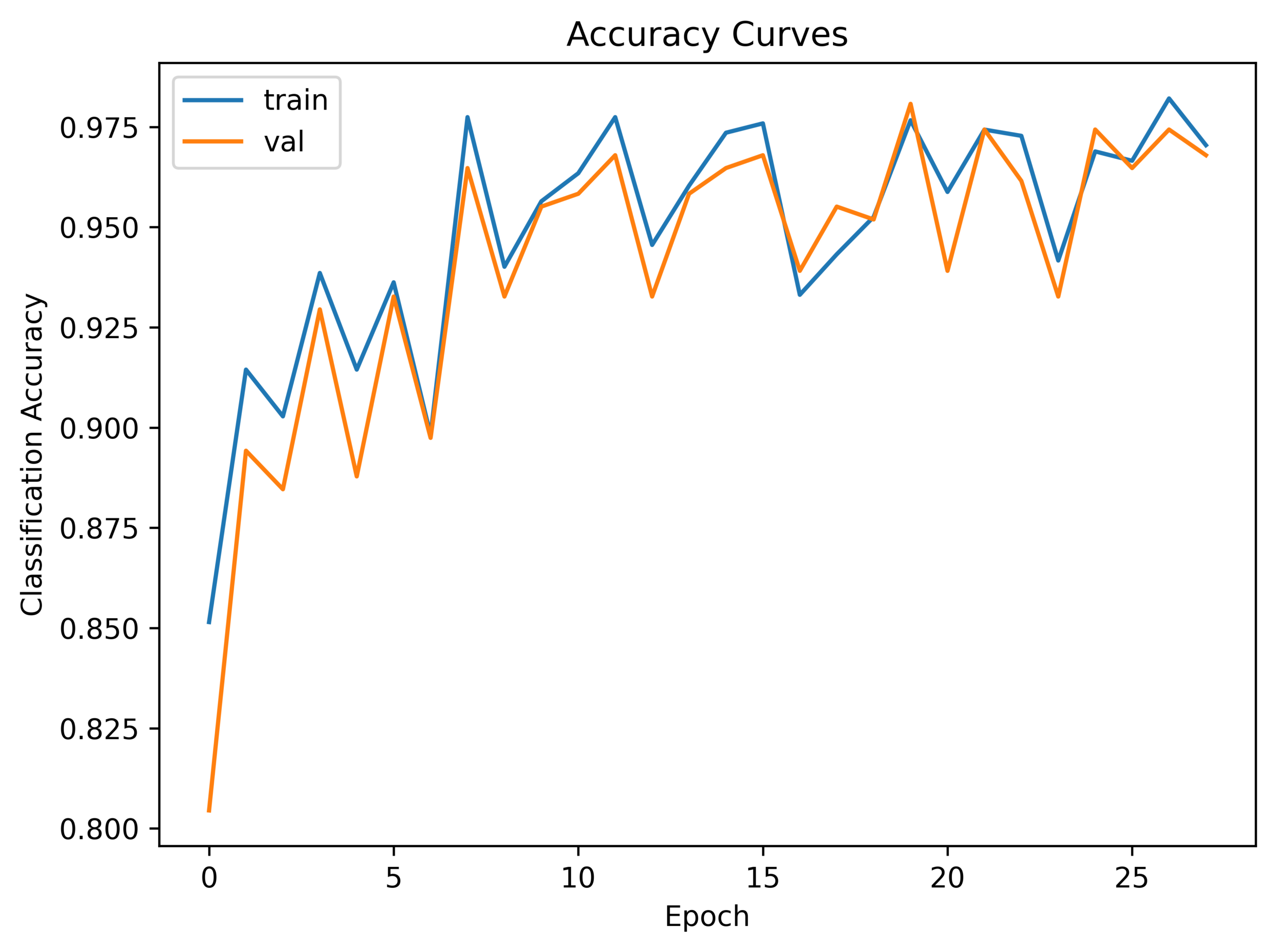
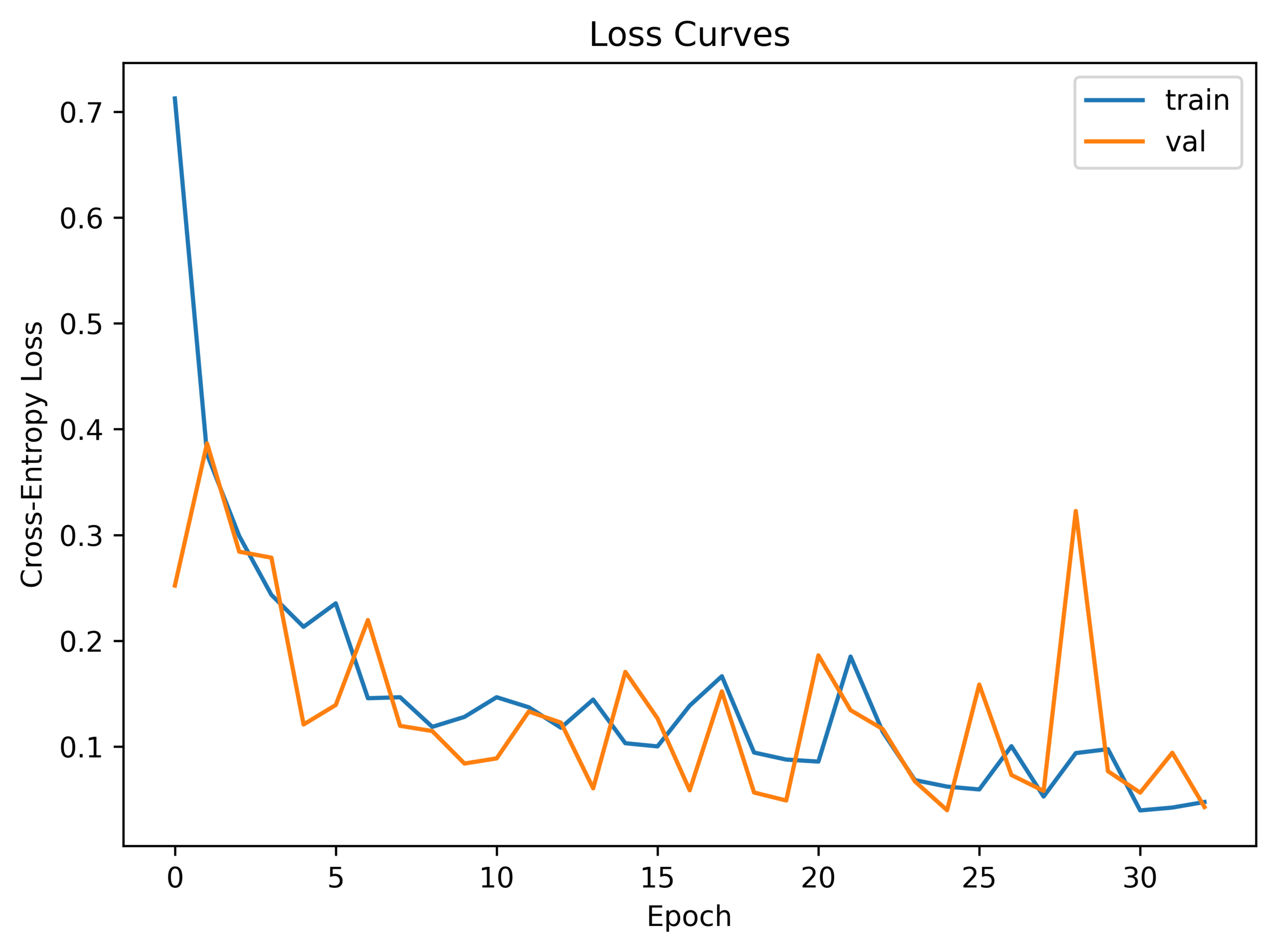
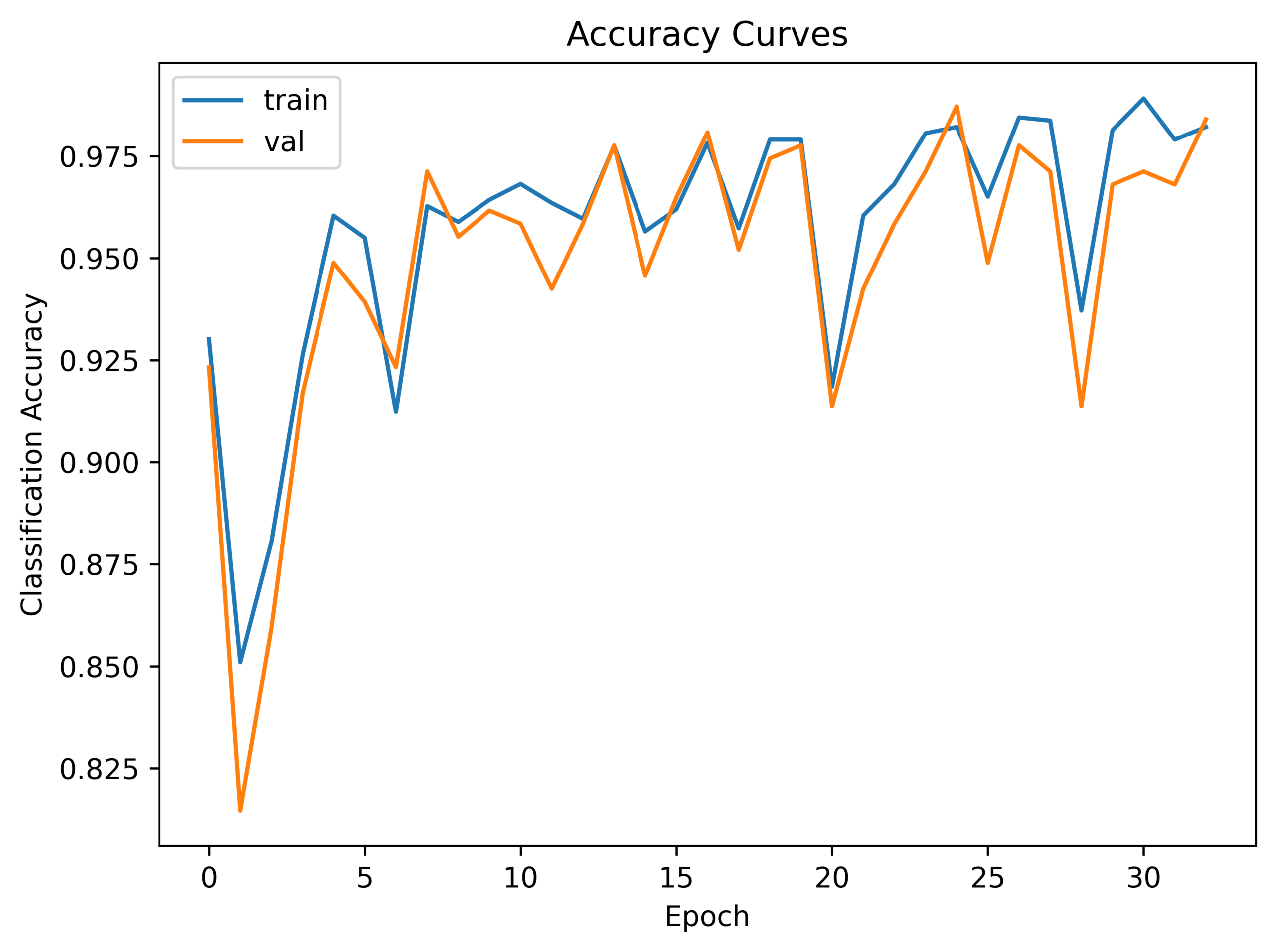
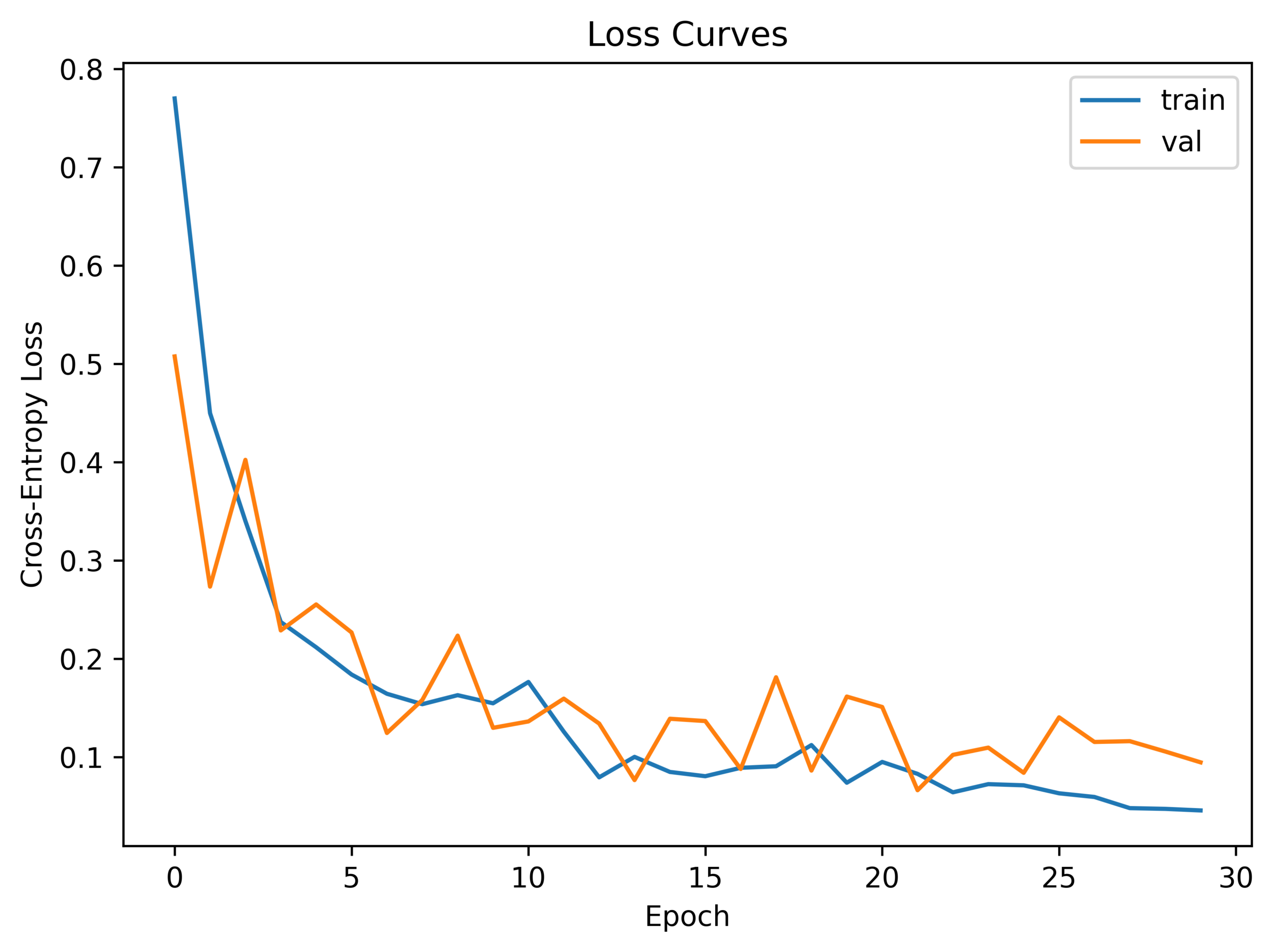
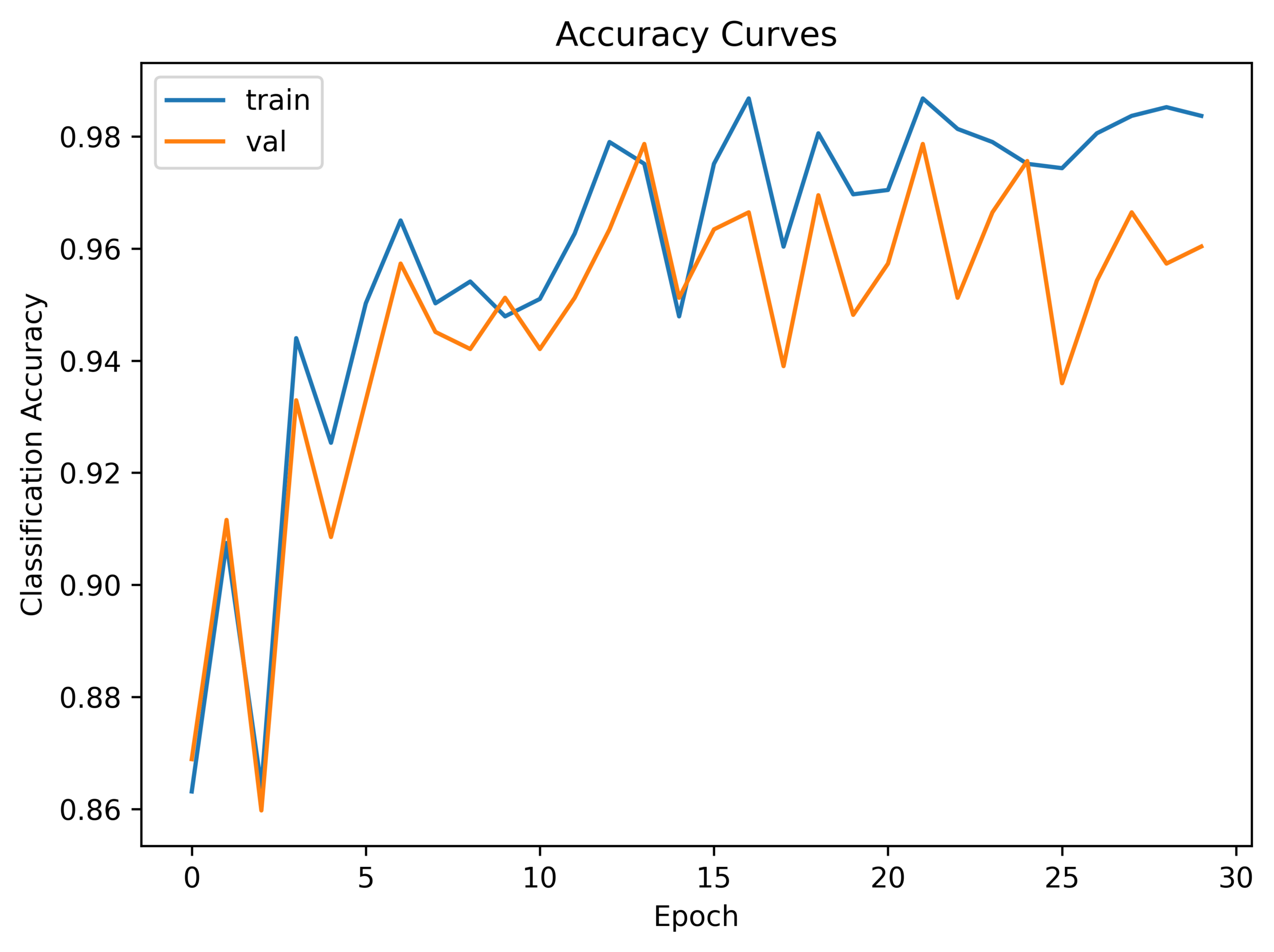
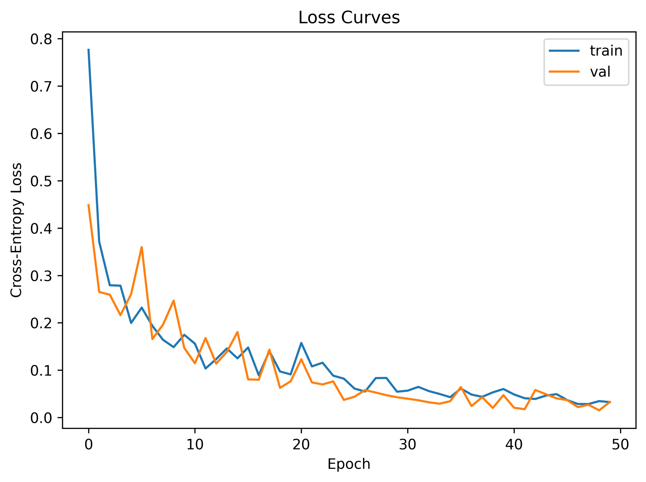
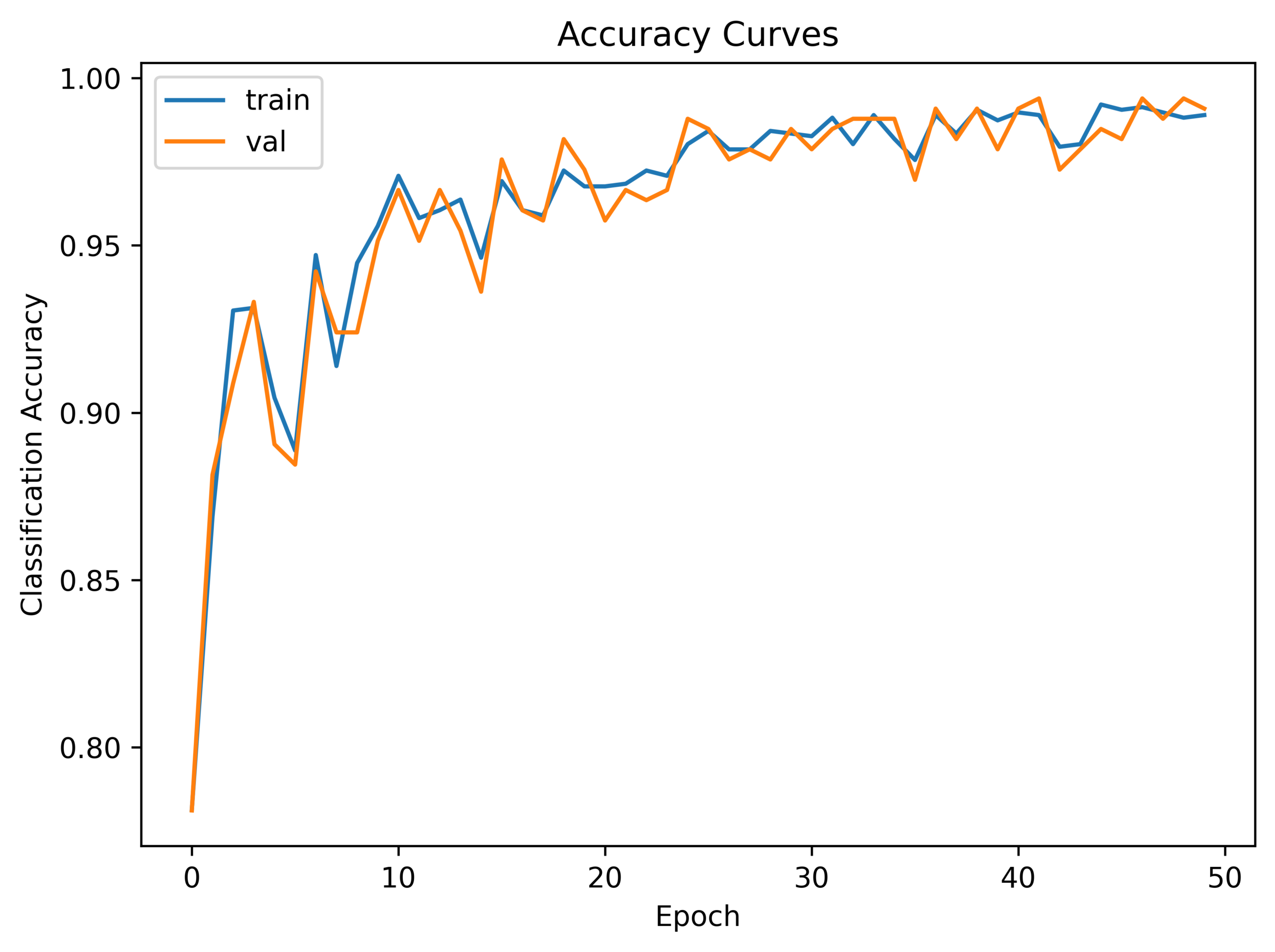
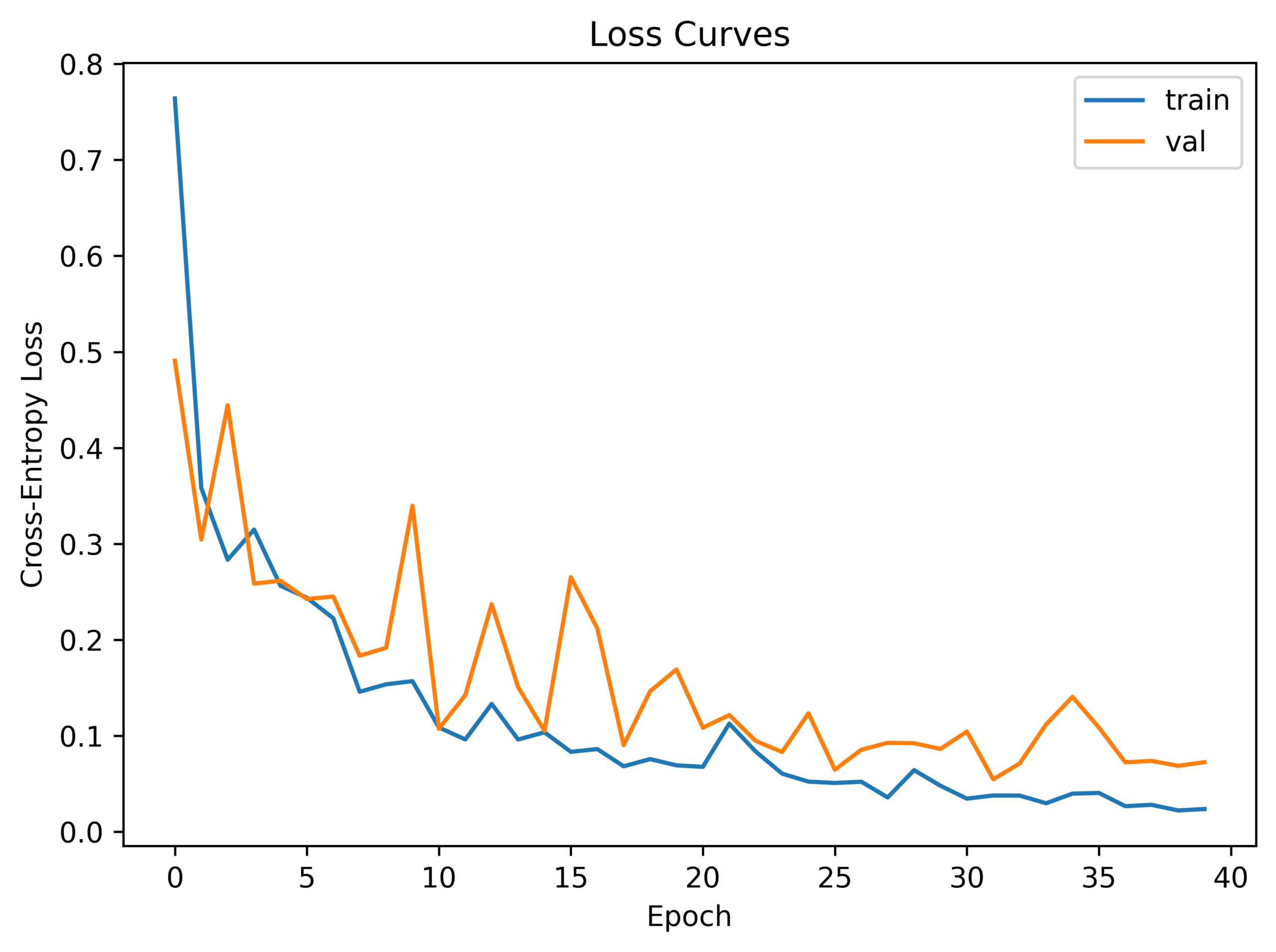
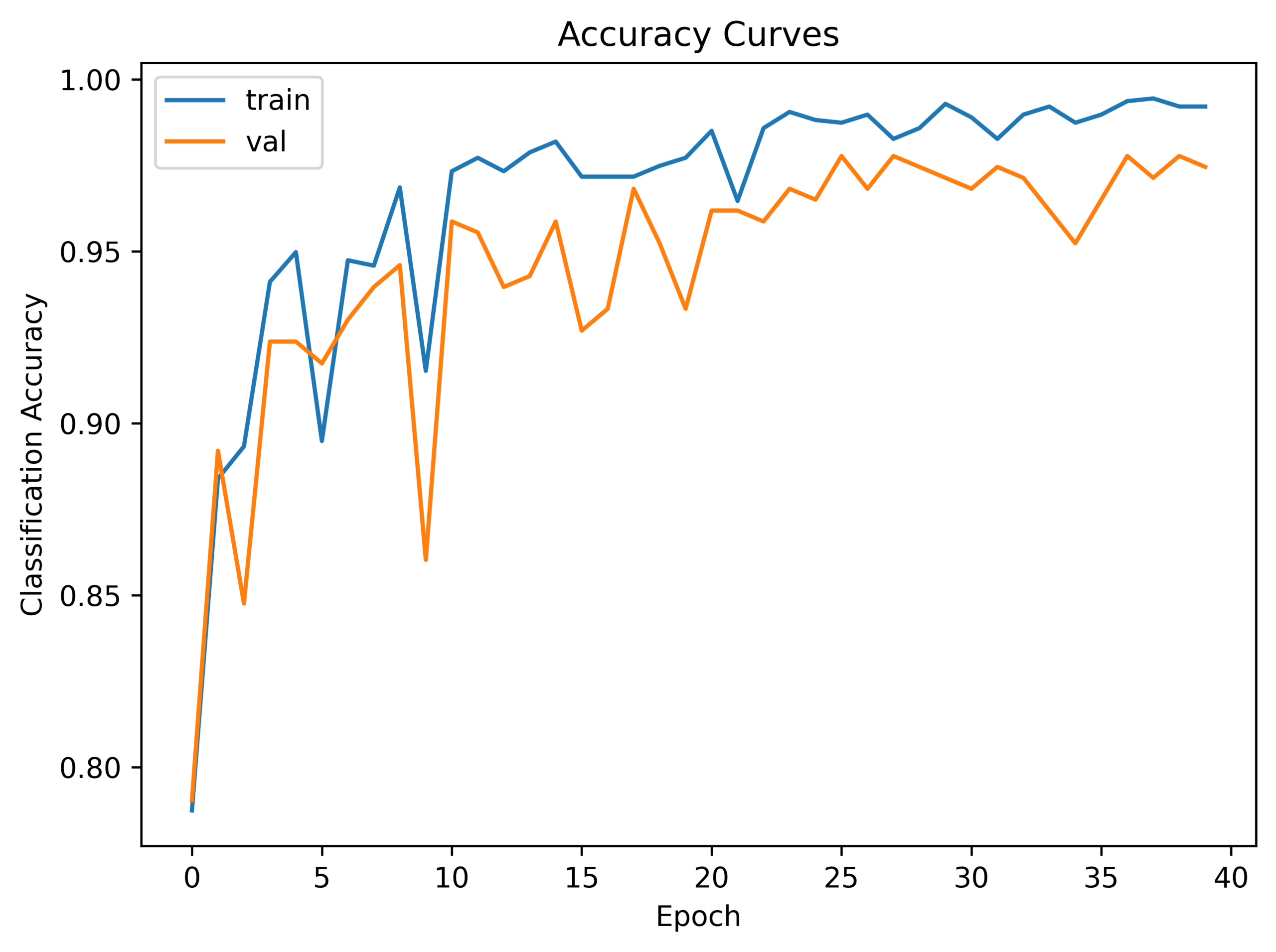
Figure 5 | Accuracy and Loss Curves of the Five Spatial Folds
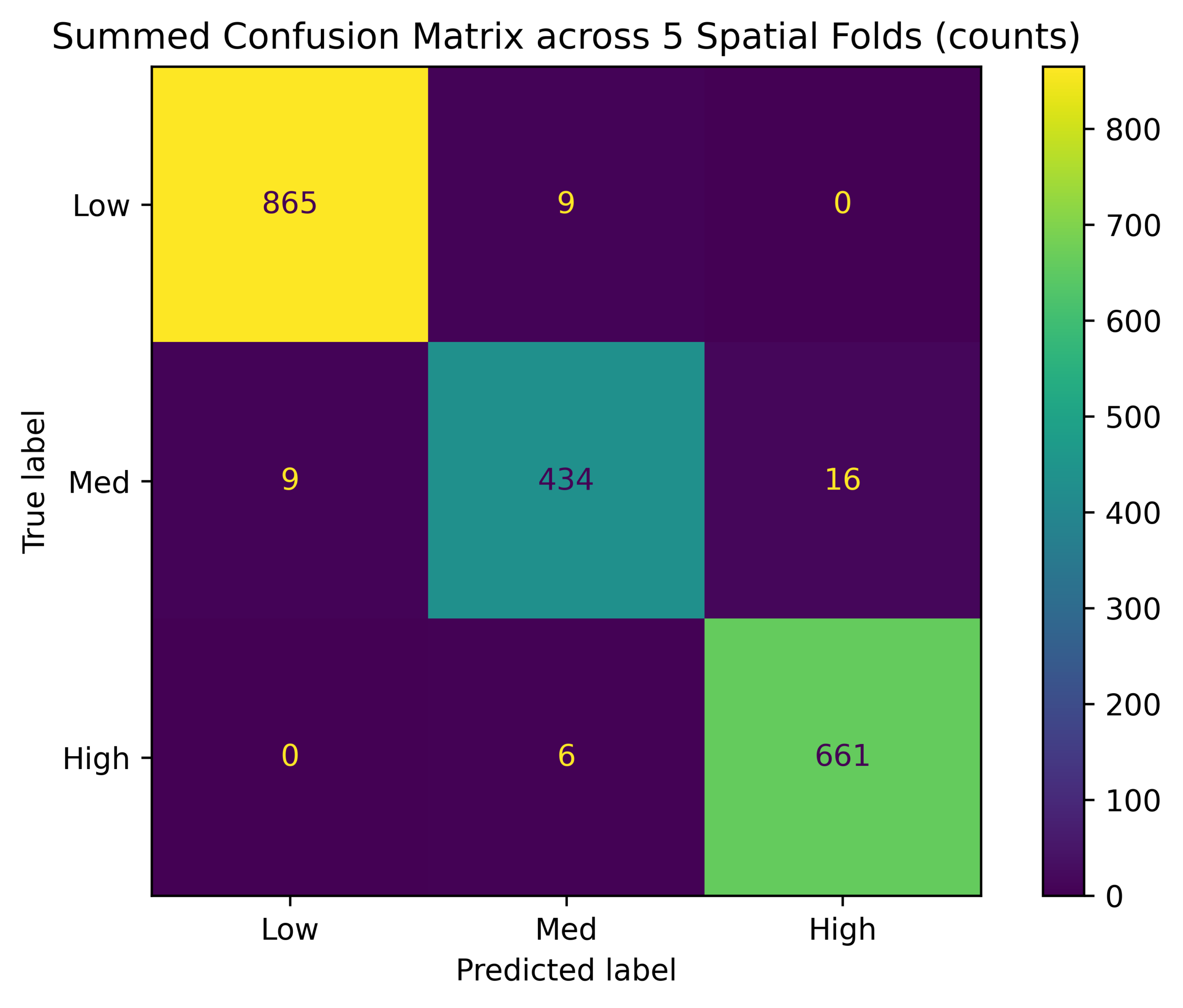
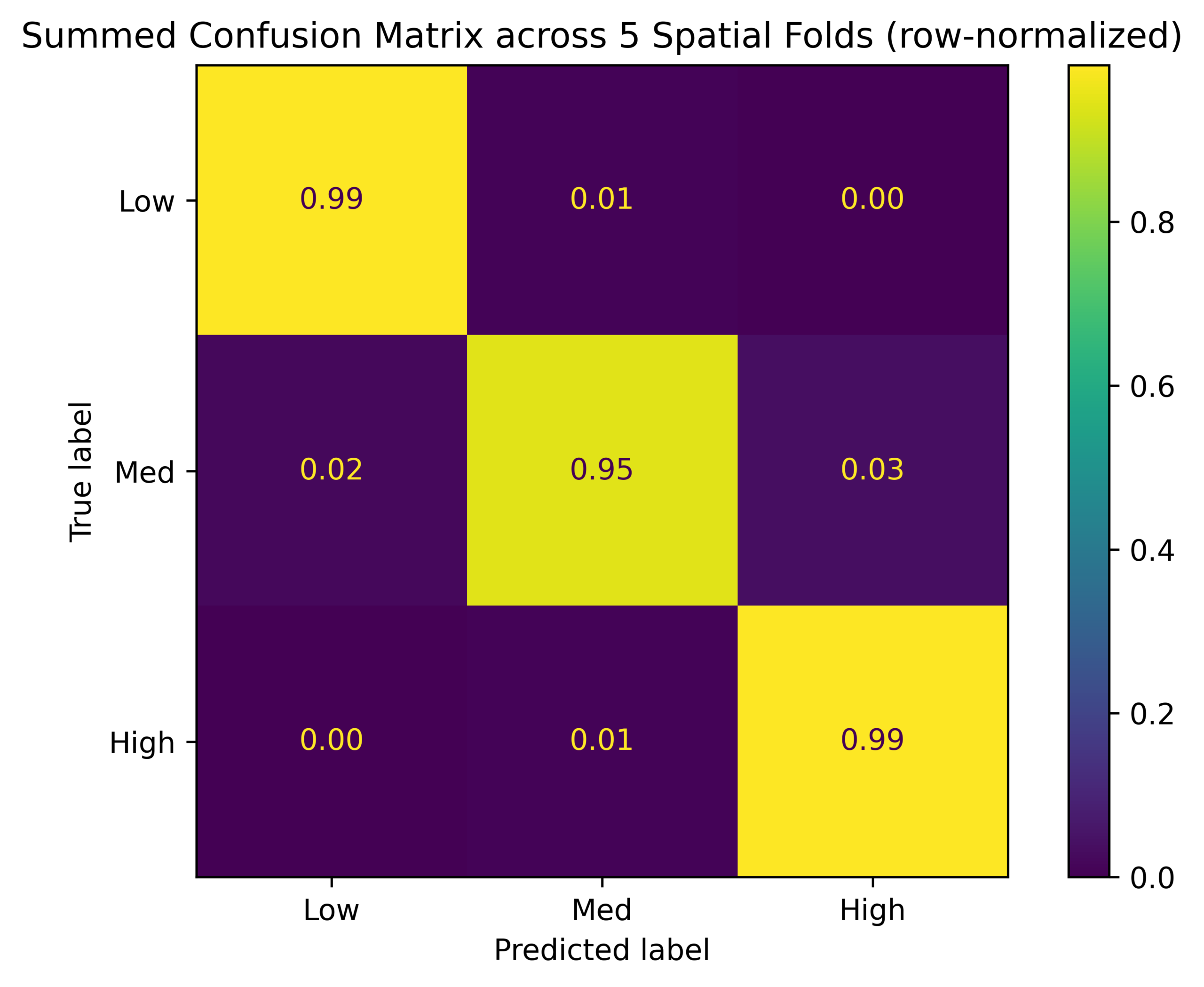
According to Table 4, the mean recall for the low suitability classification was 0.9869. The mean recall of the medium suitability class was 0.9515. This is the lowest of all classes, which means the most confusion occurs in this area. Finally, high suitability had a mean recall of 0.9894 and was very consistent across different folds. The confusion matrices in Figure 6 reinforce these results. The lower class was seldom predicted as high and vice versa. However, the medium class was sometimes predicted as high or low.
The precision for low suitability had a mean of 0.9886 and a very low variance. In the medium class, the precision had a mean of 0.9580. While this is relatively high, it is still lower than the precision for the other two classes. Finally, the high suitability class had a precision of 0.9820.
| Zero Parameter Heuristic Baseline | Random Forest Baseline | MLP Baseline | |
| Accuracy | 1.0 | 0.99502 | 0.91791 |
| Macro F1 | 1.0 | 0.99467 | 0.89928 |
| Balanced Accuracy | 1.0 | 0.99556 | 0.89476 |
A zero-parameter baseline was computed and had an accuracy, macro f1, and balanced accuracy of 1.0. A random forest on zonal statistics was also computed and had an accuracy of 0.99502, a macro f1 of 0.99467, and a balanced accuracy of 0.99556. A MLP baseline on channel means was computed and had an accuracy of 0.91791, a macro f1 of 0.89928, and a balanced accuracy of 0.89476.
| Normal CNN | Habitat Shuffled | Cultivated Shuffled | KWA Shuffled | |
| accuracy | 0.96517 | 0.93034 | 0.97263 | 0.90796 |
| macro F1 | 0.95834 | 0.92735 | 0.96751 | 0.87929 |
| balanced_accuracy | 0.95742 | 0.93255 | 0.96524 | 0.86696 |
With CNN ablation, when the habitat layer was shuffled, the accuracy went down from 0.96517 to 0.93034. When the cultivated layer shuffled, the accuracy increased from 0.96517 to 0.97263. When the KWA layer was shuffled, the accuracy decreased from 0.96517 to 0.90796.
There are few ethical concerns to this study as there are no living participants. Datasets are public and therefore have little privacy concern. However, there is an ethical issue of usage. Problems may show up if planners use the model in areas that haven’t been tested yet and overly trust the results.
Discussion
Consistently high accuracy across the folds highlights that the model generalizes well across sample spatial folds. In addition, the rapid decrease in loss during the early phases of the training, as seen in Figure 5, reveals that the model can efficiently capture strong spatial patterns within the data. Minor fluctuations in later stages of training can be attributed to spatial data variability rather than model instability. This behavior demonstrates that the model didn’t memorize tiles, and generalization remained successful. Furthermore, Moran’s I analysis suggests reduced geographic leakage between training and testing partitions. However, while the minimum training distance exceeds 1 m, neighboring areas may still have similar environmental characteristics so complete geographic independence can’t be claimed.
The sensitivity analysis shows relatively low percentages of reclassification due to moderate weight changes as seen in Table 5. While the formula is not validated, small changes have little effect on the results. This indicates that the labels are relatively stable.
Additionally, 500 tiles were overridden into becoming low suitability due to the habitat fraction rule. These 500 tiles likely come from the stratified sampling of habitat heavy locations. The override makes the dataset more conservative, turning locations that may have been classified as medium suitability into low. This creates a sharp boundary at 10% habitat, meaning the CNN partially learns a predefined rule rather than continuous ecological gradient.
The high mean recall for the low suitability class, as seen in Table 4, emphasizes that the model rarely misclassifies locations that have a lower value based on the reproduced formula. As seen in Figure 6, 862 tiles have a true low classification while 872 tiles were predicted to have a low classification, where the 10 tiles that were misclassified were of the medium suitability class.
Furthermore, the fact that the mean recall for the medium class is lower than that of the high and low classes is understandable, as the medium class consists of intermediate regions where feature distributions overlap both low and high suitability classes and scores can vary. This does bring a conceptual limitation to light in that the medium suitability class may not be implementable and learnable. In most cases, high suitability and low suitability areas will most likely be important to know for environmental planning, but medium suitability locations may not be. Finally, the high mean recall for the high suitability class suggests that the CNN can successfully reproduce the heuristic environmental scoring used to create the classes, especially that of the higher class. This relationship is reinforced in Figure 6. The confusion matrices convey that most errors occur at decision boundaries rather than flipping between opposite categories. This means that most errors occur between medium and neighboring classes rather than between extreme classes.
The high accuracy rate indicates that the classes have some separation and that the CNN can effectively capture distinct features in the environmental data. It also means that misclassification remains low within the limited environmental variables used in the study. However, other factors that may have an impact are not considered, so classification is not absolute. Since the balance accuracy is about the same as the regular accuracy, performance is not inflated by an imbalance of classes. The high metrics indicate that the CNN is good at reproducing the provided heuristic formula rather than predicting ecological suitability. In conclusion, the results demonstrate minimal evidence of overfitting, high predictive power, low variance, and stability across sampled areas.
The high precision for low suitability, as seen in Table 4, means the model is almost never wrong in predicting low suitability of a location based on the given heuristic scoring. The fact that the precision of the medium class is lower than that of the other two classes reveals that the medium class is the hardest to learn and the least stable across folds. Finally, the high value of the precision of the high suitability class conveys that the model is effective in identifying optimal locations for solar panel installation based on the given variables.
The statistics from Table 6 indicate that labels are almost perfectly recoverable from the formula that generates them. Additionally, the high values for the random forest model indicate that simple summary statistics can almost completely solve the task. The values of the MLP, while high, are not as high as the other tests. This means that though non-spatial neural features do well, spatial neural features do better.
Furthermore, the ablation test in Table 7 reveals that the CNN only partially relies on spatial structure. The performance degradation after shuffling the KWA suggests that the model uses more than just tile averages. Habitat shuffling also had a slightly degraded performance reinforcing this idea. However, the cultivated shuffling indicates that the cultivated land layer doesn’t contribute overly meaningful spatial structure. The CNN seems to rely on both summary statistics and spatial structure at varying levels.
The CNN performs well on this spatial dataset for a few reasons. First, the input channels are well structured and consistent, with each channel encoding a specific environmental feature, capturing meaningful spatial interactions across layers. Furthermore, the dataset is balanced through different quotas, which ensures that the model sees all types of patterns equally. Notably, the selected tile size captures spatial context, enabling accurate evaluation of each location.
However, there are a few limitations to these results. First, the model was mainly trained in one region of the United States. Therefore, it may not generalize well in other global locations. Moreover, the suitability labels were generated using a heuristic environmental scoring formula, rather than direct ecological ground truth. This means there can be a difference in true suitability based on the opinions of factor weights. Furthermore, the tile sampling is quota-based. This changes the natural distribution of ecosystems. When the model is actually implemented, these proportions will differ from what was tested. Another limitation is that the baseline model comparison indicates that the zero parameter heuristic and the random forest both perform well on the data, implying that a CNN may not be necessary. Additionally, the model only includes three environmental layers while additional ecological factors that may have an impact like hydrology, slopes, and wetlands are not considered. There is also a limitation in the architecture in that the CNN is relatively large compared to the dataset size. Although techniques were implemented to reduce this, the model may still be over-parameterized. Future work can compare this model against smaller CNNs to determine if it can achieve similar performance. Finally, temporal data is not considered within the model, making it potentially inaccurate in the subtleties of day-to-day changes within ecosystems.
Conclusion
This paper was able to construct a multi-channel CNN to reproduce a heuristic ecological suitability framework that evaluates solar power installation locations. The three-channel CNN uses inputs of key wildlife areas, critical habitats, and cultivated land to reach a high accuracy and reproducibility. The results indicate that the CNN can capture environmental features and distinguish between suitability classes.
This study is significant as it focuses on the environmental impact of solar panels rather than the power output or economic viability that most current models focus on. Future models can incorporate the prototype created in this study as a component to evaluate ecological suitability with other factors after additional testing. Since this CNN reproduces a given formula, it requires much more development before implementation in any planning. This prototype can be used as a pre-screening tool for solar site selection after more work is done, as there is a high recall for low suitability locations. Future work could expand on this approach by implementing temporal data, such as seasonal changes, within the model. After implementing a transfer experiment and confirming that this model can work in other locations, the framework could be incorporated into urban planning to prevent the spread into environmentally vulnerable areas. Additionally, the model could possibly be implemented in agricultural PV planning with more specific crop data and testing.
This study can become a building block of numerous new applications to reduce the environmental impact of human actions. When the world we live in is slowly changing, it is up to us to ensure that nature can still survive.
References
- EIA, “U.S. Energy Information Administration (EIA) – Ap,” Eia.gov, Apr. 25, 2024. https://www.eia.gov/environment/emissions/carbon/ [↩]
- “Global renewable capacity is set to grow strongly, driven by solar PV – News – IEA,” IEA, Oct. 07, 2025. https://www.iea.org/news/global-renewable-capacity-is-set-to-grow-strongly-driven-by-solar-pv [↩]
- P. A. Fleming, “All that glitters – Review of solar facility impacts on fauna,” Renewable and Sustainable Energy Reviews, vol. 224, pp. 115995–115995, Jul. 2025, doi: https://doi.org/10.1016/j.rser.2025.115995. [↩] [↩]
- L. Gigović, D. Pamučar, D. Božanić, and S. Ljubojević, “Application of the GIS-DANP-MABAC multi-criteria model for selecting the location of wind farms: A case study of Vojvodina, Serbia,” Renewable Energy, vol. 103, pp. 501–521, Apr. 2017, doi: https://doi.org/10.1016/j.renene.2016.11.057. [↩]
- M. A. Anwarzai and K. Nagasaka, “Utility-scale implementable potential of wind and solar energies for Afghanistan using GIS multi-criteria decision analysis,” Renewable and Sustainable Energy Reviews, vol. 71, pp. 150–160, May 2017, doi: https://doi.org/10.1016/j.rser.2016.12.048. [↩]
- Q. Yang et al., “A GIS-based high spatial resolution assessment of large-scale PV generation potential in China,” Applied Energy, vol. 247, pp. 254–269, Aug. 2019, doi: https://doi.org/10.1016/j.apenergy.2019.04.005. [↩] [↩]
- Y. Zhang, J. Ren, Y. Pu, and P. Wang, “Solar energy potential assessment: A framework to integrate geographic, technological, and economic indices for a potential analysis,” Renewable Energy, vol. 149, pp. 577–586, Apr. 2020, doi: https://doi.org/10.1016/j.renene.2019.12.071. [↩] [↩]
- D.-T. Nguyen, M.-H. Truong, and D.-T. Phan, “Gis-based simulation for solar farm site selection in south-central Vietnam,” GeoJournal, Jun. 2021, doi: https://doi.org/10.1007/s10708-021-10454-x. [↩] [↩]
- D. J. Pojadas and M. L. S. Abundo, “A spatial cost-benefit-externality modelling framework for siting of variable renewable energy farms: A case in Bohol, Philippines,” Renewable Energy, vol. 181, pp. 1177–1187, Jan. 2022, doi: https://doi.org/10.1016/j.renene.2021.09.114. [↩]
- M. Tawalbeh, A. Al-Othman, F. Kafiah, E. Abdelsalam, F. Almomani, and M. Alkasrawi, “Environmental impacts of solar photovoltaic systems: A critical review of recent progress and future outlook,” Science of The Total Environment, vol. 759, no. 143528, p. 143528, Nov. 2020, doi: https://doi.org/10.1016/j.scitotenv.2020.143528. [↩]
- A. Gasparatos, C. N. H. Doll, M. Esteban, A. Ahmed, and T. A. Olang, “Renewable energy and biodiversity: Implications for transitioning to a Green Economy,” Renewable and Sustainable Energy Reviews, vol. 70, pp. 161–184, Apr. 2017, doi: https://doi.org/10.1016/j.rser.2016.08.030. [↩] [↩]
- Kévin Barré, A. Baudouin, Jérémy S. P. Froidevaux, V. Chartendrault, and C. Kerbiriou, “Insectivorous bats alter their flight and feeding behaviour at ground‐mounted solar farms,” Journal of Applied Ecology, Dec. 2023, doi: https://doi.org/10.1111/1365-2664.14555. [↩]
- Y. Liu, C. Ding, D. Su, T. Wang, and T. Wang, “Solar park promoted microbial nitrogen and phosphorus cycle potentials but reduced soil prokaryotic diversity and network stability in alpine desert ecosystem,” Frontiers in Microbiology, vol. 13, Sep. 2022, doi: https://doi.org/10.3389/fmicb.2022.976335. [↩]
- T. Li, L. Lu, Z. Kang, H. Li, J. Wu, and W. Du, “Contrasting responses of soil bacterial and fungal networks to photovoltaic power station,” Frontiers in Microbiology, vol. 15, Dec. 2024, doi: https://doi.org/10.3389/fmicb.2024.1494681. [↩]
- Y. Li, A. Armstrong, C. Simmons, N. Z. Krasner, and R. R. Hernandez, “Ecological impacts of single-axis photovoltaic solar energy with periodic mowing on microclimate and vegetation,” Frontiers in Sustainability, vol. 6, Feb. 2025, doi: https://doi.org/10.3389/frsus.2025.1497256. [↩]
- J. Vervloesem, E. Marcheggiani, M. A. M. Choudhury, and B. Muys, “Effects of Photovoltaic Solar Farms on Microclimate and Vegetation Diversity,” Sustainability, vol. 14, no. 12, p. 7493, Jun. 2022, doi: https://doi.org/10.3390/su14127493. [↩]
- J. Li et al., “Effects of Single‐Axis and Fixed‐Tilt Photovoltaic Array Construction on the Soil Seed Bank Characteristics in Semi‐Arid Grasslands,” Land Degradation & Development, vol. 36, no. 2, pp. 478–489, Nov. 2024, doi: https://doi.org/10.1002/ldr.5372. [↩]
- S. Yue, W. Wu, B. Yuan, D. Ye, and W. Bai, “Large‐scale photovoltaic farms significantly change the vegetation diversity and biomass through influencing soil moisture and physiochemical properties,” Vadose Zone Journal, vol. 24, no. 2, Mar. 2025, doi: https://doi.org/10.1002/vzj2.70002. [↩]
- M. Graham et al., “Partial shading by solar panels delays bloom, increases floral abundance during the late-season for pollinators in a dryland, agrivoltaic ecosystem,” Scientific Reports, vol. 11, no. 1, Apr. 2021, doi: https://doi.org/10.1038/s41598-021-86756-4. [↩]
- F. Valera, L. Bolonio, A. La Calle, and E. Moreno, “Deployment of Solar Energy at the Expense of Conservation Sensitive Areas Precludes Its Classification as an Environmentally Sustainable Activity,” Land, vol. 11, no. 12, p. 2330, Dec. 2022, doi: https://doi.org/10.3390/land11122330. [↩]
- X. Song, T. Liu, G. Wang, Y. Zhang, and C. Li, “Floating photovoltaic systems homogenize the waterbird communities across subsidence wetlands in the North China Plain,” Journal of Environmental Management, vol. 349, pp. 119417–119417, Jan. 2024, doi: https://doi.org/10.1016/j.jenvman.2023.119417. [↩]
- H. Sawyer, N. M. Korfanta, M. J. Kauffman, B. S. Robb, A. C. Telander, and T. Mattson, “Trade‐offs between utility‐scale solar development and ungulates on western rangelands,” Frontiers in Ecology and the Environment, vol. 20, no. 6, pp. 345–351, Apr. 2022, doi: https://doi.org/10.1002/fee.2498. [↩]
- M. O. Levin et al., “Solar Energy-driven Land-cover Change Could Alter Landscapes Critical to Animal Movement in the Continental United States,” Environmental Science & Technology, vol. 57, no. 31, pp. 11499–11509, Jul. 2023, doi: https://doi.org/10.1021/acs.est.3c00578. [↩]
- L. Jin et al., “Photovoltaic Power Station Impacts on the Benthic Ecosystem and Sediment Carbon Storage in Tidal Flats in China,” Environmental Science & Technology, vol. 58, no. 47, pp. 20954–20967, Nov. 2024, doi: https://doi.org/10.1021/acs.est.4c04189. [↩]
- Z. Zhu et al., “The development of fishery-photovoltaic complementary industry and the studies on its environmental, ecological and economic effects in China: A review,” Energy Nexus, vol. 15, pp. 100316–100316, Jul. 2024, doi: https://doi.org/10.1016/j.nexus.2024.100316. [↩]
- J. Kiesecker, S. Baruch-Mordo, C. M. Kennedy, J. R. Oakleaf, A. Baccini, and B. W. Griscom, “Hitting the Target but Missing the Mark: Unintended Environmental Consequences of the Paris Climate Agreement,” Frontiers in Environmental Science, vol. 7, Oct. 2019, doi: https://doi.org/10.3389/fenvs.2019.00151. [↩]
- Ö. AKAR, Ekrem SARALIOĞLU, Oğuz GÜNGÖR, and Halim Ferit BAYATA, “Automatic Detection of Vineyards using machine learning and deep learning algorithms,” International journal of engineering and geosciences, vol. 9, no. 1, pp. 12–24, Feb. 2024, doi: https://doi.org/10.26833/ijeg.1252298. [↩]
- B. Austin-Gabriel, C. N. Monsalve, and Varde, Aparna S, “Power Plant Detection for Energy Estimation using GIS with Remote Sensing, CNN & Vision Transformers,” arXiv.org, 2024. https://arxiv.org/abs/2412.04986 [↩]
- J. Jeong and H. Kim, “Multi-Site Photovoltaic Forecasting Exploiting Space-Time Convolutional Neural Network,” Energies, vol. 12, no. 23, p. 4490, Nov. 2019, doi: https://doi.org/10.3390/en12234490. [↩]
- M. Vlaminck, R. Heidbuchel, W. Philips, and H. Luong, “Region-Based CNN for Anomaly Detection in PV Power Plants Using Aerial Imagery,” Sensors, vol. 22, no. 3, p. 1244, Feb. 2022, doi: https://doi.org/10.3390/s22031244. [↩]