Do Global Forest Datasets Accurately Map Mangroves in Mumbai?

Abstract

Mangroves are specialised trees that provide significant carbon storage. They also play a crucial role in shoreline stabilization and natural flood protection, especially in densely populated cities like Mumbai. However, reported estimates of mangrove extent show differences depending on the datasets and classification methods used. The purpose of this study is to evaluate the differences between Hansen Global Forest Change (GFC) and Global Mangrove Watch (GMW), so that it can be determined whether these datasets accurately represent mangroves in Mumbai. This analysis was limited to the Hansen 20N 070E tile and the merged GMW tiles N20E072 and N20E073, covering Mumbai’s mangroves and the adjacent Thane Creek system. The methodology began by reprojecting the raster datasets to the EPSG:32643 coordinate system, with GMW being used as the reference mangrove mask. Within this mask, Hansen’s treecover2000, lossyear, and gain layers were used to assess spatial agreement and forest stability. Results show that approximately 17.5% of GMW pixels is classified as persistent forest in Hansen and 82.5% as never forest, with detected loss within the mangrove mask effectively absent (14 pixels, ≈0.07 ha). This pattern suggests Hansen captures the dense interior mangrove canopy but misses the majority of GMW pixels along sparse fringes and narrow tidal channels, likely due to the 10% canopy threshold combined with optical-sensing limitations in intertidal environments. These findings suggest that Hansen and GMW disagree systematically under this workflow, though without field validation this disagreement cannot be read as evidence that either product is more accurate. Datasets such as GMW, which incorporate radar data and additional coastal constraints, may provide more direct coverage for extent mapping and for identifying mangrove zones.

Keywords: mangroves; Mumbai; Global Mangrove Watch; Hansen GFC; raster alignment; remote sensing

Introduction

Mangroves are specialised trees and shrubs that grow in saline water in intertidal zones. They have high carbon dioxide retention capabilities as well as strong, stilt-like roots that help them survive in muddy and changing water levels, making them one of the most important coastal habitats around the world.

They are extremely effective carbon sinks, storing around 1,000 tonnes of carbon per hectare. They can contain up to four times higher carbon stocks than terrestrial forests due to large underground and soil carbon pools¹.

Moreover, they act as natural coastal defenders against various climate events and calamities². In fact, a 100-metre belt of mangroves can reduce wave height by 13–66% through their dense root network’s ability to dissipate wave energy and trap sediments. This buffering effect protects against storm surges and flood risks³. Apart from this, they aid in trapping sediments, which stabilize shorelines and reduce erosion.

For densely populated coastal cities such as Mumbai, these features are extremely critical—their functions are approximately valued at ₹1,700 crore annually as reported by the Maharashtra Mangrove and Marine Biodiversity Conservation Foundation, with peer-reviewed studies further documenting the ecosystem-service value of Mumbai’s mangroves⁴, and the Thane Creek mangrove belt has been measured as having average above- and below-ground carbon densities of approximately 117–128 Mg C ha^-15. Apart from the ecological aspects, these mangroves also protect fishing communities’ livelihoods by promoting biodiversity and providing nursing grounds for fish and other marine life⁶. Overall, all the aforementioned functions of mangroves make them indispensable for the environment, especially in the case of Mumbai itself.

Mumbai, one of India’s most densely populated cities, contains one of the largest urban mangrove covers in the world. These are spread all around the periphery of Mumbai, with the majority of mangroves being concentrated in Thane creek, Mahim, Versova, and Gorai⁷. The reported total cover varies due to varying mapping methods, but recent studies show Greater Mumbai’s mangrove cover is around 50–70 km², while the Mumbai suburban district contributes around 64 km² of mangroves⁸. The Thane Creek Sanctuary is the largest protected mangrove region in the area, with a reported site area of around 65 km² according to one source, and 90 km² according to another. This disagreement may be an effect of how boundaries are defined (such as the inclusion/exclusion of areas enclosed within mangroves)⁸.

However, despite their importance, Mumbai’s mangroves have faced continuous threats of destruction, fragmentation, or thinning from many different angles. Due to rapid urbanization in Mumbai, projects such as the Coastal Road and other industrial developments, together with illegal encroachment, have contributed to mangrove loss and fragmentation. Moreover, recurring issues as a result of weak regulatory enforcement including untreated sewage discharge and illegal waste dumping have degraded the water and land where mangroves usually thrive, hence posing a threat to their health. Rapid climate change, sea-level rise, and the increased frequency of extreme rainfall alter the habitat of mangroves irreparably, further worsening this crisis.

Numerous studies have attempted to quantify the exact changes of mangrove cover in Mumbai, but most have varying results based on spatial extent, time frame, as well as resolution of imaging. Some studies that employ satellite imagery (Landsat or Sentinel data) have reported local increases or even doubling of mangrove cover in parts of Thane Creek from 79.14 km² in 1990 to 154.5 km² in 2017, attributed to the deposition of sediment that has allowed mangroves to spread closer to the center of the creek^7,9. In contrast, some other studies report marginal declines or near stability in total mangrove cover over multiple decades, with the total mangrove area in Mumbai being 50.52 km² in 2004, and 48.7 km² in 2013¹⁰. More recent satellite-based assessments using machine-learning classifiers and high-resolution imagery have continued to refine these estimates^11,12. These contrasting findings are likely due not only to differences in the spatial scales analyzed but also to the datasets and classification methods employed.

This study focuses on a comparison of mangrove datasets in Mumbai using two major global datasets: Hansen Global Forest Change (GFC) and Global Mangrove Watch (GMW). The scope of this paper is limited to evaluating spatial agreement, temporal detection behavior, and classification stability of areas within Mumbai’s coastal regions. Additionally, the research does not attempt to quantify actual area loss, or to model future scenarios, but rather focuses on how dataset choice can influence interpretation of both extent and persistence in these surrounding regions.

One potential limitation of this study is that it is constrained to Mumbai and its surrounding coastal mangrove areas. For the analysis, we used: the Hansen 20N 070E tile and the merged GMW tiles N20E072 and N20E073, which covered the majority of mangroves found surrounding Mumbai’s urban area and Thane Creek. Some mangroves near the very edges of these tiles may fall outside the aligned analysis grid, which is noted as a minor scope limitation. Because the study covers a relatively small area, its findings provide useful insights into dataset performance in this coastal context. However, they cannot be directly generalized to other mangrove systems because of differences in canopy structure, sediment characteristics, tidal cycles, and climate. Moreover, Mumbai itself is a unique coastal ecosystem considering that it is one of the few metropolitan cities surrounded by mangroves. Therefore, its ecology differs from other such systems.

Additionally, the comparative analysis is limited to two widely used datasets: Hansen Global Forest Change (GFC) and Global Mangrove Watch (GMW). Although these are among the most commonly referenced datasets for most use cases because they combine multiple satellite data sources, other high-resolution or region-specific datasets were not included in this paper such as ESA WorldCover¹³, or the JAXA ALOS PALSAR dataset¹⁴. As a result, the conclusions only reflect agreement and disagreement between these two datasets do not represent all available mangrove- or forest-monitoring products.

Dataset	Description	Strengths	Limitations
Hansen Global Forest Change15	-Not mangrove-specific -30 m resolution using NASA/USGS Landsat data(Optical Imagery) -Defines trees as vegetation with canopy cover above 10%(the threshold used in this study) -Uses decision tree classification to classify trees	-Annual dataset -High-resolution forest loss data	-Optical imagery may be affected by cloud cover and tidal variation. The classification may also confuse mangroves with other forest types.
Global Mangrove Watch16	-Mangrove-specific -10 m resolution using ALOS PALSAR, ESA WorldCover, Landsat(radar and optical imagery) -Classifies mangroves based on intertidal forests in coastal regions -Uses object based classification as well as radar texture	-High reported accuracy in published validation(94.0% accuracy)16 due to object based classification and radar and optical (cloud and tidal effects have less influence on the data)	-Not strictly annual dataset

Methods

Study Area

The study is focused on the mangrove ecosystems within the Mumbai region in India. The analysis was restricted to the tile corresponding to 20N, 70E in the Hansen dataset, with the mangrove mask defined from the corresponding GMW tiles (N20E072 and N20E073, merged). This tile encompasses the majority of the mangrove cover surrounding Mumbai, including Thane Creek, Mahim, Versova, and Gorai. All spatial analyses were conducted at the pixel level within this defined region.

Hansen Global Forest Change (GFC)

The Hansen Global Forest Change (GFC) product is a general forest temporal dataset derived mainly from Landsat optical imagery with a 30 m resolution, which maps tree cover and annual loss/gain using canopy cover and height thresholds¹⁵. Since it does not explicitly separate mangroves from other forest or wetland vegetation, it is more susceptible to the effects of cloud cover, mixed coastal pixels, and flooding, leading to the omission or misclassification of mangroves.

In this dataset, forest is defined as vegetation with more than 10% canopy cover. The GFC layers used in this study are: tree cover baseline (treecover2000), which records the percentage canopy cover for each pixel as of the year 2000; loss year (lossyear), which encodes the calendar year a pixel transitioned from forest to non-forest as integers from 1 (corresponding to 2001) through 24 (corresponding to 2024), with 0 meaning no detected loss; and forest gain (gain), a binary flag marking pixels classified as gaining forest cover between 2000 and 2012. The first and last reflectance composite bands provided in the GFC product were not used in the temporal analysis because they contain Landsat reflectance values rather than annual forest-state data.

Global Mangrove Watch (GMW)

The GMW dataset provides a spatially explicit binary classification of mangrove extent. GMW is a mangrove-specific spatial dataset that integrates radar data (ALOS PALSAR) with optical imagery and coastal habitat masks, allowing it to more accurately detect mangroves in waterlogged, intertidal environments¹⁶. The Global Mangrove Watch v3 dataset (2020 epoch) was used in this study¹⁷; the two tiles N20E072 and N20E073 were merged before analysis to cover the full Mumbai coastline and Thane Creek system. GMW itself is not free of error: published validations note omission and commission errors of narrow or fragmented mangrove patches, increased uncertainty in disturbed or intertidal regions, and artefacts introduced by sensor limitations, which can lead to under- or over-counting of mangrove pixels in some regions^17,18. Due to their unique techniques of collecting data, including differences in sensor type (only optical vs radar+optical), classification thresholds, spatial resolution, and ecological constraints, there are often discrepancies between the two.

In this study, the GMW was the reference mask used to define the spatial extent within which all subsequent analyses were performed, not as a validated ground truth. Unlike GMW, the Hansen dataset does not distinguish mangroves from other forest types. It detects tree cover based on spectral classification and canopy thresholds.

Raster Preprocessing and Spatial Alignment

All raster preprocessing was performed using Python, primarily with the Rasterio, NumPy, and pyproj libraries^19,20,21,22. The Hansen GFC analysis covers the period from 2000 to 2024, set by the treecover2000 baseline and the 2024 release of the lossyear band.

A major issue in comparing the datasets is that they use different coordinate reference systems (CRS). This makes it difficult to conduct a direct comparison between the two datasets. Thus, we first projected both datasets onto a common projected coordinate system: EPSG:32643 (UTM Zone 43N).

This projection was selected because it is appropriate for western India and allows accurate area calculations in meters. Reprojection was performed using nearest-neighbor resampling to preserve categorical integrity of forest and mangrove classifications.

Subsequently, we aligned the two grids to allow for a pixel-level comparisony. The GMW raster was resampled to match the Hansen grid so that each pixel represented the same geographic area across datasets.

Then the pixel area was calculated for both datasets using the relation: Pixel area (m²) = |pixel width × pixel height|. Join this section to the preceding sentence: “Pixel area was calculated using |pixel width × pixel height|, and area in hectares was calculated as Area (ha) = (pixel count × pixel area in m²) / 10,000. All statistics in the Results section come from this calculation.

Nodata pixels in treecover2000 and lossyear were treated as zero after masking to the GMW extent. Pixels where the GMW mask was zero or nodata were excluded from all calculations.

A mask was created from the merged GMW tiles to restrict all analysis to mangrove pixels. Within this mask, three pixel classes were derived from the GFC layers. Pixels with treecover2000 below 10% and gain equal to 0 were classified as never forest. Pixels with treecover2000 at or above 10% and lossyear equal to 0 were classified as persistent forest, since they were forested in 2000 with no detected loss. Pixels with treecover2000 at or above 10% and lossyear greater than 0, or where gain equalled 1 and lossyear was greater than 0, were classified as temporary forest. In this classification, never forest represents pixels that Hansen did not identify as canopy, persistent forest captures stable canopy across the record, and temporary forest captures pixels with detected loss at some point.

In compact form:
never forest := treecover2000 < 10 AND gain == 0
persistent forest := treecover2000 ≥ 10 AND lossyear == 0
temporary forest := (treecover2000 ≥ 10 AND lossyear > 0) OR (gain == 1 AND lossyear > 0)

To quantify agreement between datasets, three spatial comparisons were computed: the count of mangrove pixels within the GMW mask that Hansen also classified as forest, the count of mangrove pixels within the GMW mask that Hansen did not classify as forest, and the count of Hansen forest pixels falling outside GMW mangrove areas. These are summarized both visually and numerically in the Results section.

Results

After reprojection and grid alignment to the Hansen 30 m resolution grid (EPSG:32643), the total mangrove area within the study region was calculated as approximately 12,852 hectares (ha) based on the merged Global Mangrove Watch (GMW) mask. This figure exceeds Mumbai-specific mangrove cover estimates of 50–70 km² cited in some sources because the merged GMW tiles also include adjacent mangrove systems along Thane Creek and the broader Konkan coastline within the analysis region. All subsequent forest detection analysis was restricted to these mangrove-classified pixels.

These results show that Hansen classifies approximately 17.5% (2,251.96 ha) of GMW pixels as persistent forest and 82.5% (10,600.34 ha) as never forest. Furthermore, the spatial visualizations show clear areas where Hansen detects forest outside GMW mangroves and vice versa. Put together, these findings suggest that Hansen detects a stable persistent core within the GMW mask but consistently misses the majority of GMW-classified pixels, particularly along sparse fringe and edge areas. The disagreement is consistent with the limitations of optical sensing in intertidal environments.

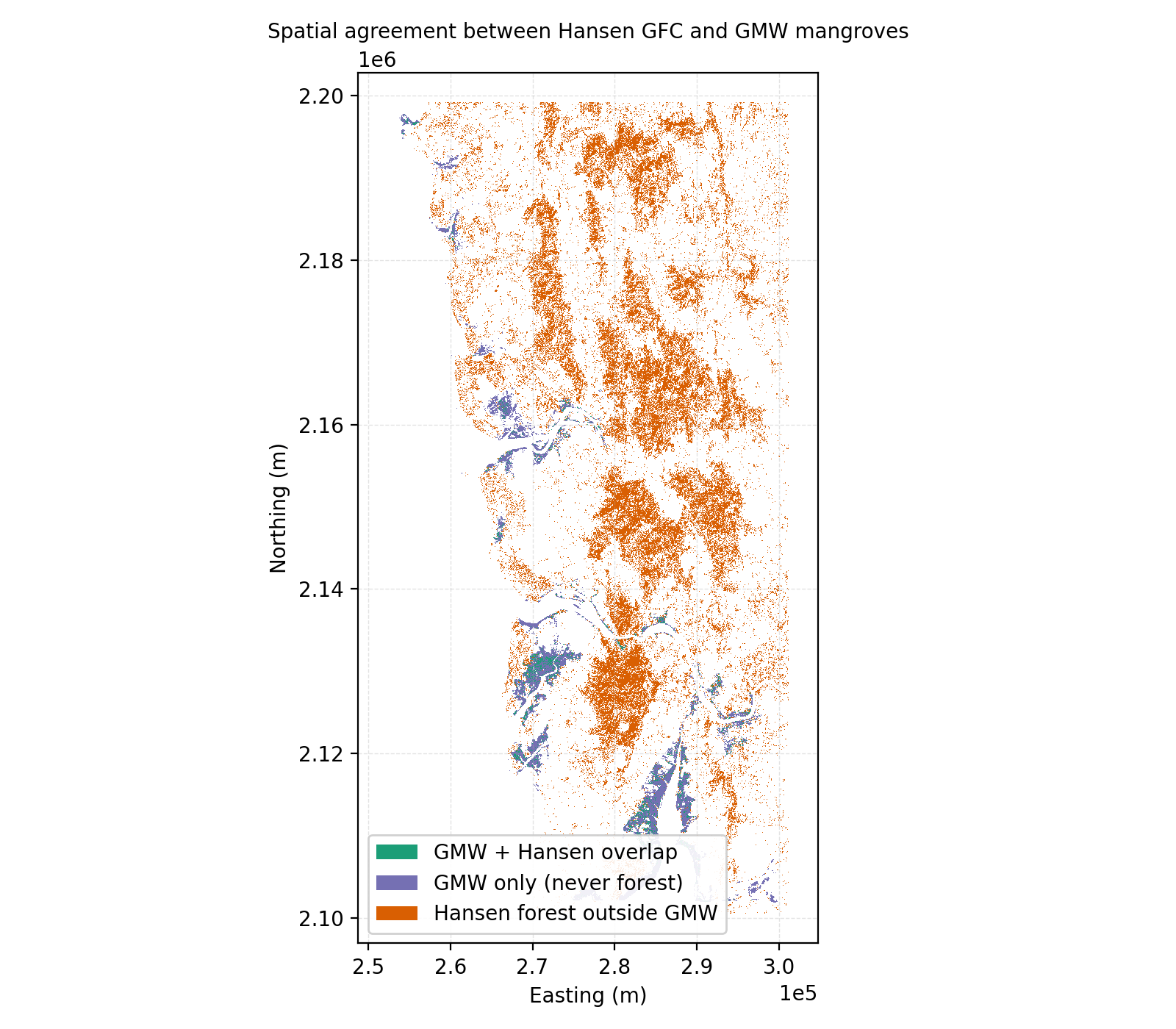
Class	Area (ha)	% of GMW total
GMW only (mangrove pixels not detected as forest by Hansen)	10,600.34	82.5%
GMW + Hansen overlap (mangrove pixels detected as forest by Hansen)	2,251.96	17.5%
Hansen only (forest pixels outside the GMW mask)	≈8.1 × 10	not directly comparable

The Hansen-only area covers the entire 10°×10° tile and largely reflects non-mangrove forest cover across the broader Konkan and Western Ghats region; it is reported here for completeness but is not directly comparable to the GMW mangrove extent.

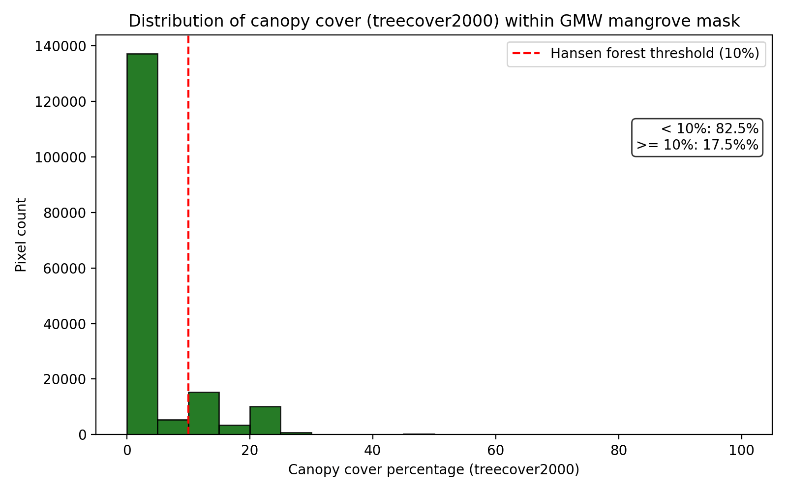
In terms of the classification of mangroves within the GMW mask, the results show approximately 2,251.96 ha (17.5%) of pixels are classified as persistent forest by Hansen — pixels that crossed the 10% canopy cover threshold in 2000 and showed no detected loss through 2024. Approximately 10,600.34 ha (82.5%) are classified as never forest, meaning Hansen’s treecover2000 layer never registered them as forest under the 10% canopy threshold and no gain was recorded. The median canopy cover within the GMW mask is 0% and the mean is 3.27%, with 82.5% of pixels falling below the 10% threshold (Figure 2), confirming that the disagreement is driven by the threshold itself rather than by sensor instability over time.

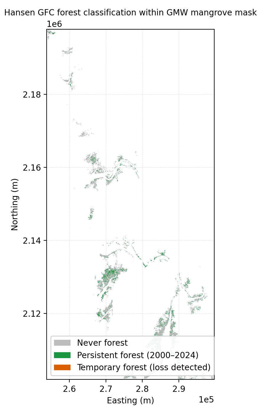
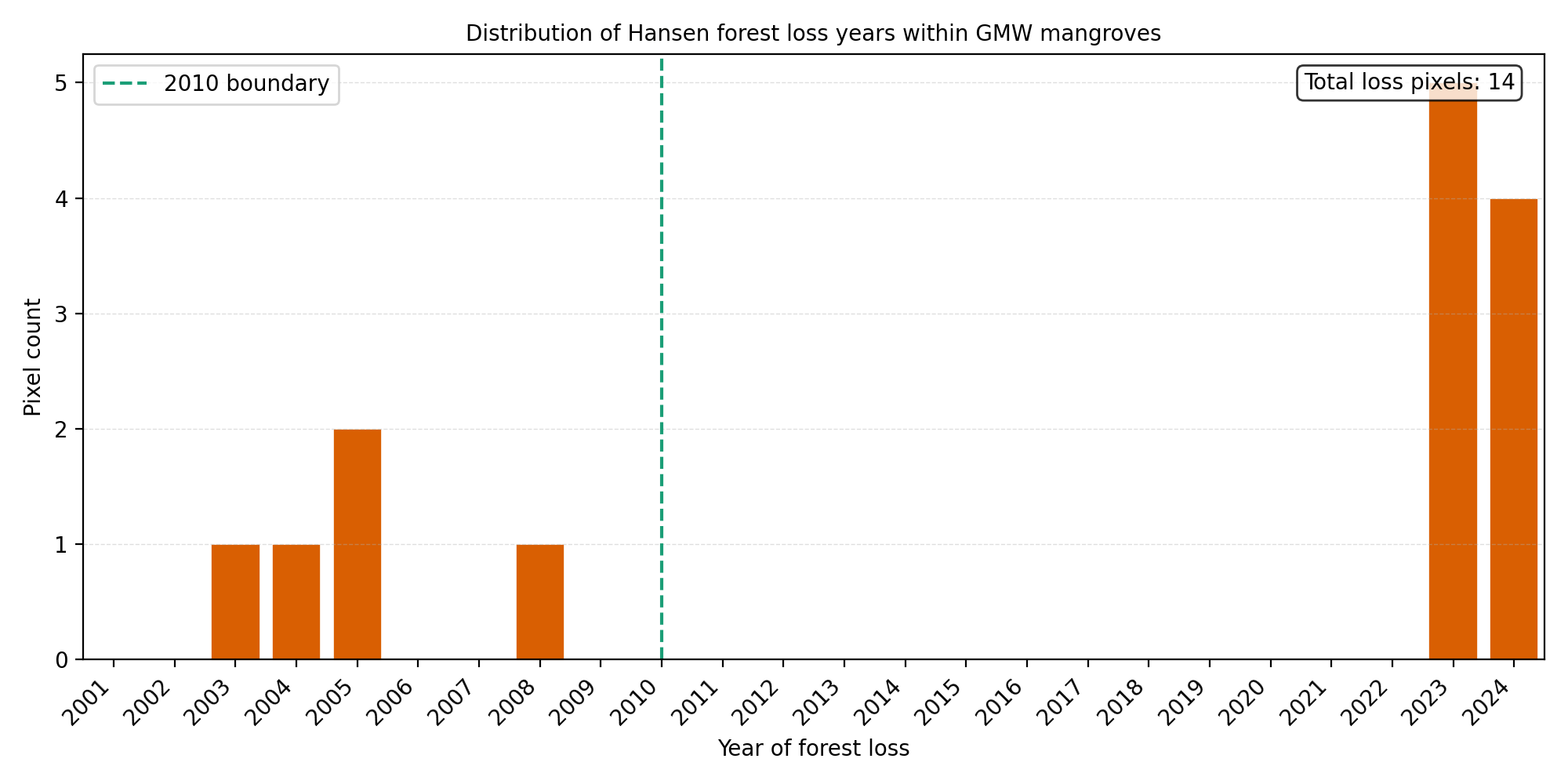
Temporary forest pixels are essentially absent in the dataset: only 14 pixels (≈0.07 ha) within the entire GMW mask have a detected loss event between 2001 and 2024. As a category, temporary forest contributes negligibly to the analysis (less than 0.001%) and is best read as scattered noise at 30 m resolution rather than as evidence of meaningful mangrove loss.

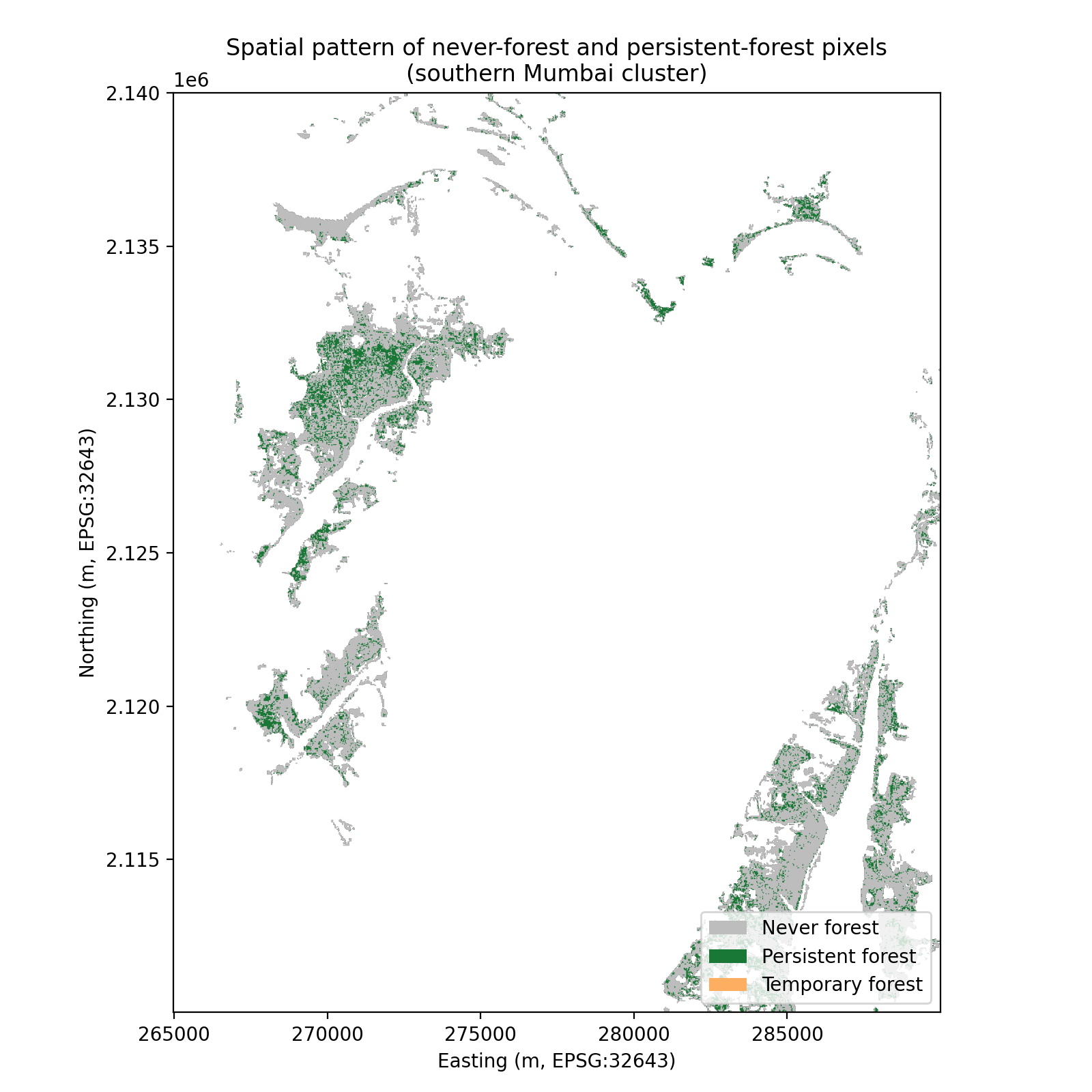
Together, these results suggest that Hansen detects a stable persistent core of mangrove canopy within the densest creek clusters, while systematically missing the majority of GMW-classified pixels. The class map (Figure 3) and a zoom into the southern Mumbai cluster (Figure 4) show that never-forest pixels are concentrated along creek edges, narrow tidal channels, and sparse outer-fringe areas where canopy density is below the 10% threshold, rather than in dense mangrove cores. This pattern is consistent with the optical-sensing limitations described earlier, not with widespread mangrove loss.

The temporal distribution of the few detected loss events is shown in Figure 5. Of the 14 loss pixels, 5 (36%) have a recorded loss year in 2003–2008 and 9 (64%) in 2023–2024; the median loss year is 2008. Given the small absolute count, this distribution is best interpreted as scattered noise rather than systematic forest loss within the GMW mask.

These results indicate that Hansen’s forest classification is internally consistent across the GMW mask—pixels above the canopy threshold remain classified through 2024—but the threshold itself excludes the majority of pixels GMW identifies as mangrove. The disagreement between the two products therefore reflects a difference in detection sensitivity rather than temporal instability of the forest signal.

Discussion

Although approximately 17.5% of mangrove pixels are classified as persistent forest in Hansen, the fact that 82.5% is not classified as forest suggests that Hansen’s forest definition does not consistently capture mangrove ecosystems under its 10% canopy threshold. This disagreement appears to reflect a difference in detection sensitivity rather than large-scale mangrove loss, as cumulative loss within the mangrove mask was minimal over the study period.

Disagreement between Hansen and GMW is expected because the datasets are designed for different purposes and are built from different sensors and classification assumptions. Hansen Global Forest Change is a general-purpose forest monitoring product derived primarily from Landsat optical imagery and canopy cover thresholds. In contrast, GMW is designed specifically for mangroves and integrates radar (ALOS PALSAR) with optical imagery and coastal habitat constraints to improve detection in intertidal environments.

Several factors can plausibly explain why Hansen misses the majority of GMW-classified pixels. Mangroves occur in intertidal zones where the observed surface reflectance changes substantially with tidal stage²³. Even if vegetation is unchanged, the mixture of water, mudflat, and canopy within a pixel can vary across images, causing unstable classification at 30 m resolution.

Additionally, mangrove canopy structure is often heterogeneous and can be sparse or low in height compared to many inland forests. Pixels with canopy cover near a fixed threshold (e.g., 10%) may move above or below the detection boundary due to seasonal effects, partial inundation, atmospheric conditions, or mixed-pixel effects²⁴.

Moreover, optical imagery is sensitive to cloud cover and haze, which can reduce usable observations and increase uncertainty in coastal regions. Radar-based inputs in GMW are less affected by cloud cover and can better discriminate against vegetated surfaces in wet environments, contributing to higher classification stability^25,26.

These factors jointly suggest that Hansen’s forest detection signal may reflect canopy threshold sensitivity as much as ecological structure when applied to mangroves.

A critical interpretation point is that “never forest” in this analysis does not necessarily represent the absence of mangroves. Instead, it indicates that Hansen does not detect canopy at that pixel under its 10% threshold. Therefore, the observed dominance of never-forest classifications should be interpreted as a limitation of applying a general forest product to coastal wetland vegetation, not as evidence that mangroves are absent from these areas.

This distinction is important because Hansen products are frequently used in environmental monitoring workflows and policy discussions. If mangroves are frequently mischaracterized as non-forest, conclusions about mangrove extent or change derived from Hansen alone may be biased.

Mangroves are increasingly treated as natural infrastructure due to their role in coastal protection and flood risk reduction. For cities such as Mumbai, mangrove mapping supports environmental impact assessment, coastal regulation compliance, and resilience planning. The results here imply that dataset choice can strongly influence interpretation of mangrove extent and change.

Specifically, Hansen-derived forest detection metrics may underrepresent mangrove extent in intertidal environments . However, since this study does not include field validation, the disagreement between the two products under this workflow does not establish that one is more accurate than the other. GMW-style mangrove-specific products, which incorporate radar and coastal constraints, may be better suited to baseline extent mapping and identifying mangrove zones for planning purposes. This study has several limitations. It focuses on a single geographic region (Mumbai) and a limited spatial tile. Results may not directly generalize to mangroves with different canopy structures, sediment regimes, tidal ranges, or climatic conditions. This analysis compares only two widely used datasets. Additional datasets (e.g., ESA WorldCover mangrove classes or regionally validated mangrove maps) could provide further context. The comparison framework also has a temporal mismatch: GMW v3 represents a single 2020 epoch baseline, while the Hansen analysis covers 2000–2024 through the treecover2000 baseline and the lossyear band. The two products are therefore being compared across different temporal references, and the persistence findings should be read with this design constraint in mind. Finally, this study does not include field validation. Instead, it focuses on internal consistency and comparative behavior between datasets. These results should therefore be read as a caution about dataset choice, rather than a comprehensive assesement of mangrove change in Mumbai.

Overall, the results suggest that Hansen Global Forest Change detects a stable persistent core of canopy within Mumbai’s mangroves but misses the majority of GMW-classified pixels under its 10% canopy threshold. The disagreement between Hansen and GMW is systematic and likely driven by sensor modality differences, intertidal mixed-pixel effects, and threshold-based classification limitations. Since this study does not include field validation, these findings show product disagreement under the workflow used here rather than relative accuracy of either product. They nonetheless suggest that mangrove monitoring should account for the design assumptions of any single-source forest dataset.

Acknowledgments

I would like to thank the project supervisors for guidance on project design, methodology, and paper editing. I also thank the developers and maintainers of the Global Mangrove Watch and Hansen Global Forest Change datasets for making their data publicly available. This work used open-source Python tools including Rasterio, NumPy, Pandas, Matplotlib, and related geospatial libraries for data processing and visualization.

References

1. D. C. Donato, J. B. Kauffman, D. Murdiyarso, S. Kurnianto, M. Stidham, M. Kanninen. Mangroves among the most carbon-rich forests in the tropics. Nature Geoscience. Vol. 4, pg. 293–297, 2011, https://doi.org/10.1038/ngeo1123. [↩]
2. UN Environment Programme. Mangrove forests. https://www.unep.org/topics/ocean-seas-and-coasts/blue-ecosystems/mangrove-forests, 2023. [↩]
3. A. McIvor, I. Möller, T. Spencer, M. Spalding. Reduction of wind and swell waves by mangroves. https://elaw.org/resource/reduction-of-wind-and-swell-waves-by-mangroves, 2023. [↩]
4. M. Everard, R. R. S. Jha, S. Russell. The benefits of fringing mangrove systems to Mumbai. Aquatic Conservation: Marine and Freshwater Ecosystems. Vol. 24, pg. 256–274, 2014, https://doi.org/10.1002/aqc.2433. [↩]
5. S. G. Singh, A. Vennila, R. Singh, V. S. Bharti, S. P. Shukla, C. S. Purushothaman. Standing carbon stock of Thane Creek mangrove ecosystem: An integrated approach using allometry and remote sensing techniques. Regional Studies in Marine Science. Vol. 67, pg. 103207, 2023, https://doi.org/10.1016/j.rsma.2023.103207. [↩]
6. Food and Agriculture Organization of the United Nations. The world’s mangroves 1980–2005. https://www.fao.org/4/a1427e/a1427e00.htm, 2007. [↩]
7. NASA Earth Observatory. Monitoring Mumbai’s mangroves. https://science.nasa.gov/earth/earth-observatory/monitoring-mumbais-mangroves-91333/, 2017. [↩] [↩]
8. Forest Survey of India. India state of forest report 2017 — mangrove cover chapter. Ministry of Environment, Forest and Climate Change, Government of India, Dehradun, 2018, https://fsi.nic.in/isfr2017/isfr-mangrove-cover-2017.pdf. [↩] [↩]
9. A. A. S., G. L., M. K. R., R. C., S. John, S. G., J. Thomas. Multi-decadal changes of mangrove forest and its response to the tidal dynamics of Thane Creek, Mumbai. Journal of Sea Research. Vol. 180, pg. 102162, 2022, https://doi.org/10.1016/j.seares.2021.102162. [↩]
10. A. Abhyankar, T. Sahoo, B. Seth, P. Mohapatra, S. Palai, P. Bhargava, S. Chaurasiya, S. Isasare. Mapping and change detection of mangroves around Mumbai using remote sensing and geographic information systems (GIS). Journal of Civil Engineering, Science and Technology. Vol. 12, 2021, https://doi.org/10.33736/jcest.3339.2021. [↩]
11. S. Sawant, P. Bonala, A. Joshi, M. Shindikar, A. Patil, S. Vyas, D. Deobagkar. Integration of machine learning and remote sensing for assessing the change detection of mangrove forests along the Mumbai coast. Journal of Earth System Science. Vol. 133, pg. 237, 2024, https://doi.org/10.1007/s12040-024-02378-0. [↩]
12. P. Nagarajan, L. Rajendran, N. D. Pillai, G. Lakshmanan. Comparison of machine learning algorithms for mangrove species identification in Malad creek, Mumbai using WorldView-2 and Google Earth images. Journal of Coastal Conservation. Vol. 26, pg. 44, 2022, https://doi.org/10.1007/s11852-022-00891-2. [↩]
13. ESA WorldCover. WorldCover. 2021, https://esa-worldcover.org/en. [↩]
14. Japan Aerospace Exploration Agency (JAXA). ALOS-2 / PALSAR-2. 2014, https://www.eorc.jaxa.jp/ALOS-2/en/about/palsar2.htm. [↩]
15. M. C. Hansen, P. V. Potapov, R. Moore, M. Hancher, S. A. Turubanova, A. Tyukavina, D. Thau, S. V. Stehman, S. J. Goetz, T. R. Loveland, A. Kommareddy, A. Egorov, L. Chini, C. O. Justice, J. R. G. Townshend. High-resolution global maps of 21st-century forest cover change. Science. Vol. 342, pg. 850–853, 2013, https://doi.org/10.1126/science.1244693. [↩] [↩]
16. P. Bunting, A. Rosenqvist, R. M. Lucas, L. M. Rebelo, L. Hilarides, N. Thomas, A. Hardy, T. Itoh, M. Shimada, C. M. Finlayson. The Global Mangrove Watch — A new 2010 global baseline of mangrove extent. Remote Sensing. Vol. 10, pg. 1669, 2018, https://doi.org/10.3390/rs10101669. [↩] [↩] [↩]
17. P. Bunting, A. Rosenqvist, L. Hilarides, R. M. Lucas, N. Thomas, T. Tadono, T. A. Worthington, M. Spalding, N. J. Murray, L.-M. Rebelo. Global mangrove extent change 1996–2020: Global Mangrove Watch Version 3.0. Remote Sensing. Vol. 14, pg. 3657, 2022, https://doi.org/10.3390/rs14153657. [↩] [↩]
18. P. Bunting, A. Rosenqvist, L. Hilarides, R. M. Lucas, N. Thomas. Global Mangrove Watch: Updated 2010 mangrove forest extent (v2.5). Remote Sensing. Vol. 14, pg. 1034, 2022, https://doi.org/10.3390/rs14041034. [↩]
19. C. R. Harris, K. J. Millman, S. J. van der Walt, R. Gommers, P. Virtanen, D. Cournapeau, E. Wieser, J. Taylor, S. Berg, N. J. Smith, R. Kern, M. Picus, S. Hoyer, M. H. van Kerkwijk, M. Brett, A. Haldane, J. Fernández del Río, M. Wiebe, P. Peterson, P. Gérard-Marchant, K. Sheppard, T. Reddy, W. Weckesser, H. Abbasi, C. Gohlke, T. E. Oliphant. Array programming with NumPy. Nature. Vol. 585, pg. 357–362, 2020, https://doi.org/10.1038/s41586-020-2649-2. [↩]
20. S. Gillies. Rasterio: Geospatial raster I/O for Python. https://rasterio.readthedocs.io, 2013. [↩]
21. PROJ contributors. PROJ coordinate transformation software library. https://proj.org, 2023. [↩]
22. J. D. Hunter. Matplotlib: A 2D graphics environment. Computing in Science & Engineering. Vol. 9, pg. 90–95, 2007, https://doi.org/10.1109/MCSE.2007.55. [↩]
23. T. A. Worthington, P. S. E. zu Ermgassen, D. A. Friess, K. W. Krauss, C. E. Lovelock, J. Thorley, R. Tingey, C. D. Woodroffe, P. Bunting, N. Cormier, D. Lagomasino, R. Lucas, N. J. Murray, W. J. Sutherland, M. Spalding. A global biophysical typology of mangroves and its relevance for ecosystem structure and deforestation. Scientific Reports. Vol. 10, pg. 14652, 2020, https://doi.org/10.1038/s41598-020-71194-5. [↩]
24. K. A. C. Gasparini, C. H. L. Silva Junior, Y. E. Shimabukuro, E. Arai, L. E. O. C. e Aragão, C. A. Silva, P. L. Marshall. Determining a threshold to delimit the Amazonian forests from the Tree Canopy Cover 2000 GFC data. Sensors. Vol. 19, pg. 5020, 2019, https://doi.org/10.3390/s19225020. [↩]
25. A. Ghorbanian, S. Ahmadi, M. Amani, A. Mohammadzadeh, S. Jamali. Mangrove ecosystem mapping using Sentinel-1 and Sentinel-2 satellite images and random forest algorithm in Google Earth Engine. Remote Sensing. Vol. 13, pg. 2565, 2021, https://doi.org/10.3390/rs13132565. [↩]
26. N. J. Murray, T. A. Worthington, P. Bunting, S. Duce, V. Hagger, C. E. Lovelock, R. Lucas, M. I. Saunders, M. Sheaves, M. Spalding, N. J. Waltham, M. B. Lyons. High-resolution mapping of losses and gains of Earth’s tidal wetlands. Science. Vol. 376, pg. 744–749, 2022, https://doi.org/10.1126/science.abm9583. [↩]