NHSJS Reports

Examining Median Hourly Wage Differences Between Housed and Homeless Workers Through Descriptive Analysis

August 13, 2026

Abstract

This observational and cross-sectional study aims to examine the correlation between housing status and hourly wages within the United States, using public microdata from the American Community Survey through IPUMS from 2018 to 2023, while controlling for education, race, sex, and age. Housing inequality is a rising issue in the United States that inhibits a person’s economic mobility and opportunities due to a variety of factors such as the COVID-19 pandemic and growing inflation costs. Access to stable housing is heavily linked to economic opportunity, but not much is known about how housing instability relates to labor market effects among working individuals. Using a survey-weighted regression model and descriptive statistics in computational analysis, we compared the hourly wages of individuals. Environments Python and R were used to clean, weight, and compute additional interaction testing and regression to produce results. The results of the research suggest that homeless workers earn approximately 26% less hourly wages than housed workers. This relates housing status to the economic growth of working individuals.

Keywords: Homelessness, Wages, Wage Inequality, Statistical Analysis, Housing, Data Analysis

Introduction

Our research hopes to identify any potential wage disparities between working individuals that align with past research. Previous work at the University of Chicago in 2021 has identified and categorized patterns among homeless individuals, including identifying a wage difference between unsheltered and sheltered individuals. The study understands that low wages, informal employment, and job turnover seem to be contributing to low income levels. The study has also used administrative data to recognize the health, geographic mobility, income, etc., of homeless people to create accurate poverty estimates and understand the economic well-being of homeless populations on a national level, revealing key findings regarding SNAP benefits and employment¹. While we hope that our research complements the prior findings done, our study focuses clearly on the assessment of wage disparities between homeless and housed working individuals to identify differences through the lens of labor economics by using data analysis and a regression model.

Recognizing homelessness as a problem is crucial to shaping public policy that helps reduce the rise of homelessness. In recent years, impacts of the COVID-19 pandemic and rising housing costs have resulted in people experiencing housing insecurity, with millions of people facing eviction and feeling cost-burdened. During the pandemic, approximately 580,466 Americans had been experiencing homelessness, with 27% of individuals being classified as chronically homeless by the U.S. Department of Housing and Urban Development². By 2023, the number of homeless individuals had increased by 12.5%, roughly 653,104 homeless Americans and 29.5% of more Americans experiencing chronic homelessness³. With already pre-existing barriers and rising populations that may lack public assistance and affordable healthcare, unstable housing further reduces the opportunities for economic mobility in the labor market that offer better living situations because of inequality and low wages. While many misconceptions regarding the difficulty of homelessness still exist today, low-income workers often fall into homelessness because stagnant or low wages are outpaced by rising housing costs. This creates a cycle rooted in systemic issues, leading to obstacles such as poor health, minimal healthcare, and limited employment opportunities.

Investigating whether a difference between the wages of homeless workers and housed workers exists could potentially improve policy design that combats homelessness. In this research, we aim to use data analysis to compare wages and identify any differences. We used the data gathered from the American Community Survey through IPUMS to filter years 2018-2023 on individuals ages 18-64 in the United States. However, the data excluded unsheltered homelessness due to American Community Survey data only containing individuals living in group quarters as homeless⁴^,⁵.

This study is based on a framework of labor economics, in which wages are determined by human capital, education, and skill, but also by several factors that influence decision-making. Human capital theory suggests that individuals gain employment through greater experience and productivity; however, it’s important to recognize that several types of discrimination could influence the decision of employers, some of them being affected by economic motivation and others through personal views. Employers commonly practice statistical discrimination, which focuses on hiring candidates who consist of the characteristics of a certain applicant pool, limiting mobility for other applicants who vary from those characteristics⁶. Examples of statistical discrimination include education, age, race, experience, etc. Such discrimination leads to labor market segmentation where hiring preference creates a primary sector and a secondary sector. Labor market segmentation is defined as a process where political and economic forces create a dual market separated by different characteristics, creating a primary sector that has stable wages and job ladders, while the secondary sector has unstable wages, few job ladders, and is mostly filled with minorities⁷. The segmentation into a dual market creates a mobility barrier that prevents employees from accessing employment in the other sector, leading to a difference in wage distributions for different workers⁸. Connecting back to housing status, it has been shown that the hiring standards that employers seek also include stable housing. According to a previous study focusing on homeless individuals’ obstacles and potential solutions to fix discrimination at Yale, research revealed that the most common barrier to stable employment for homeless individuals is the difficulty in gaining stable housing, where employers reject several candidates due to the lack of permanent housing⁹. Many employers associate a lack of permanent residence with a lack of adequate transportation, recognizing it as a large hindrance and preventing homeless individuals from pursuing further job opportunities due to discouragement. In this case, a permanent residence is typically a hiring standard and a positive signal that prevents employers from immediately rejecting a candidate, which creates two different markets with a primary sector consisting of housed individuals and a secondary sector with homeless individuals. While stable housing is the hiring standard that leads to the creation of dual labor markets, there are several other relevant obstacles that exist even after a previously homeless individual gains an address. It’s important to recognize obstacles such as substance use, mental health struggles, and sensitive information that still prevent individuals from gaining employment opportunities even after having a stable residence¹⁰. Although a residence removes the primary barrier for employment, such obstacles might still ensure a dual labor market.

Based on this framework, a regression model was run to identify a potential wage disparity among housed and homeless workers and, more importantly, to recognize if it’s statistically significant. It was also included with covariates such as race, sex, age, education, and survey year due to previous research demonstrating that these factors influence wage determination and labor market opportunities. Interaction analyses were additionally conducted to evaluate whether the association between homelessness and hourly wages differed across subgroups and over time, with statistically significant trends. In this study, we used Python packages for data cleansing and visualization in the form of graphs, where variables like race, education, and sex were transformed into dummy variables. Then, our regression model was run on the cleaned data to analyze if the comparison of wages done was significant or due to chance.

For this study, our primary variable was the group quarters variable, which identified an individual’s living situation according to the American Community Survey. From the IPUMS’s category labels, Group Quarter codes 1, 2, 3, and 5 represent households under the 1970 definition, households under the 1990 definition, institutions, and households under the 2000 definition, respectively, while code 4 represents other, noninstitutionalized or household group quarters such as homeless shelters, college housing, and motels. Group Quarters code 6 is not in our data and is considered a fragment, meaning that people who have previously not been included in the survey have been gathered in one category in 1850 – 1930s¹¹. Following the U.S. Department of Housing and Urban Development’s definition, a person is considered homeless if they lack a regular nighttime residence, such as living in a primary residence that is a space not meant for inhabitation or a space designed for temporary living¹². This allows us to categorize Group Quarter codes 1, 2, 3, and 5 as “housed” as they are identified as individuals with households by the American Community Survey, but also because some individuals live in a group living arrangement managed by larger facilities. Since these larger facilities provide people with a regular nighttime residence and are under the care of the institutions, we can consider them not homeless. According to the direct definition from the American Community Survey, these institutions include correctional facilities, juvenile facilities, nursing facilities, and other healthcare facilities, implying that individuals among these institutions have reliable care and are under the custody of another facility¹³.

However, a limitation arises when using this GQ code because of the non-institutional Group Quarter code 4, which encompasses a set of living arrangements such as military barracks, student housing, emergency shelters, religious housing, and more¹³. Since Group Quarter code 4 contains several non-institutional living arrangements other than homeless shelters and homeless living arrangements, the results of this study are made to be used as an estimate due to potential noise that comes with wages and data from the other groups. Another similar limitation is the American Community Survey’s inability to survey homeless individuals that don’t reside in shelters due to reasons of accessibility. The American Community Survey has been known to exclude domestic violence shelters, soup kitchens, and other non-sheltered locations where vulnerable populations reside, making the results of this study less general to the broader homeless population¹⁴. This could restrict the applicability of the findings as workers in these group quarters are not included in the wage comparisons.

Methodology

This observational and cross-sectional study uses data from a survey conducted by the U.S. Census Bureau from the American Community Survey attained through the Integrated Public Use Microdata Series (IPUMS). The American Community Survey is a nationwide survey that provides insight about the American population, including the United States and Puerto Rico. This survey gathers demographic factors, including education, income, gender, employment status, etc., through a multistage systematic design that samples a few U.S. counties in the course of a year and across 31 selected sample sites¹⁵. Approximately 3.5 million people are sampled each year, in which the survey gathers demographic data and applies weights in order to create an accurate representation of the data in regard to the greater population¹⁶. The weights are essential tools that adjust the presence of a group in accordance with the overall population and are necessary for readjusting oversampled or undersampled groups in the sample. The American Community Survey provides individual data in which, through RStudio and Python code, we analyze trends and a potential association between housing stability and wages from employers. To make the survey data more accessible and understandable, we cleaned the data through several steps and restricted the age to 18-64 years old. Since the study is focused on employed individuals in the labor market, the range is necessary to represent the standard working-age population in the United States, whose employment effects may differ.

Including variables such as race, sex, and education in our analysis and modeling is crucial to this study, as we cannot clearly state that housing stability has an effect on wages without taking into account confounding variables that alter outcomes. After acquiring the data, cleaning processes, weighting methods, a sensitivity analysis, interaction tests, and a regression model have been applied.

Cleaning the data

The first step after gathering our data was to clean the data in order to identify whether a difference exists using comparison through data visualization with accurate values. We cleaned the data to remove unsuitable individuals from the samples, such as unemployed people and people with missing values and extreme wages.

Since our study focuses on the wage difference among homeless and unsheltered working individuals, we cleaned the data for working individuals. According to the codebook extract, people with the variable “EMPSTAT” set to 1 show employment, while “EMPSTAT” set to 0 indicates unemployment in the survey. Therefore, we kept people who had the “EMPSTAT” variable (employment status) equal to 1 instead of 0. Next, we took the “AGE” variable in the data and made sure that the sample only contained individuals ages 18-64 for employed workers.

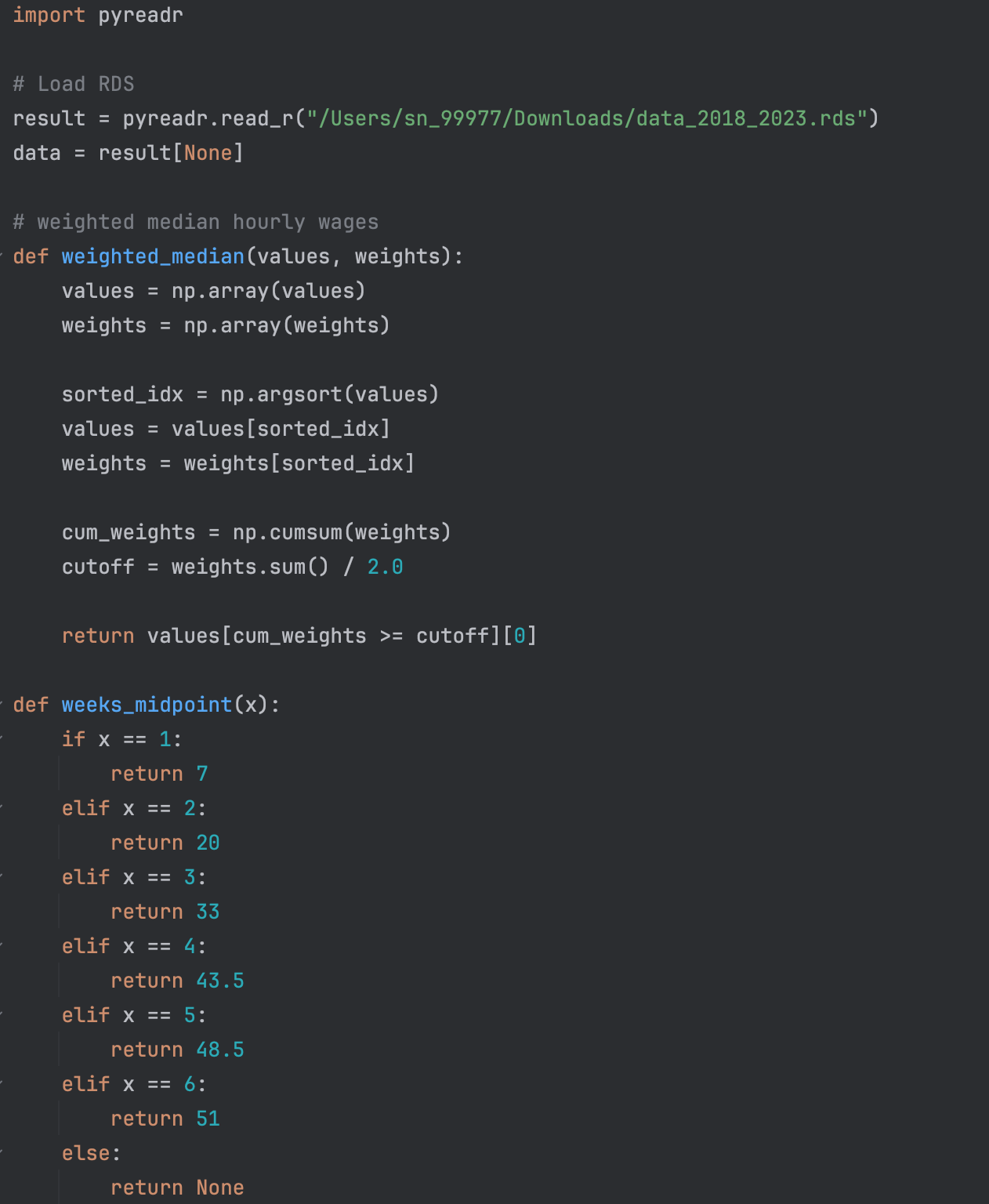
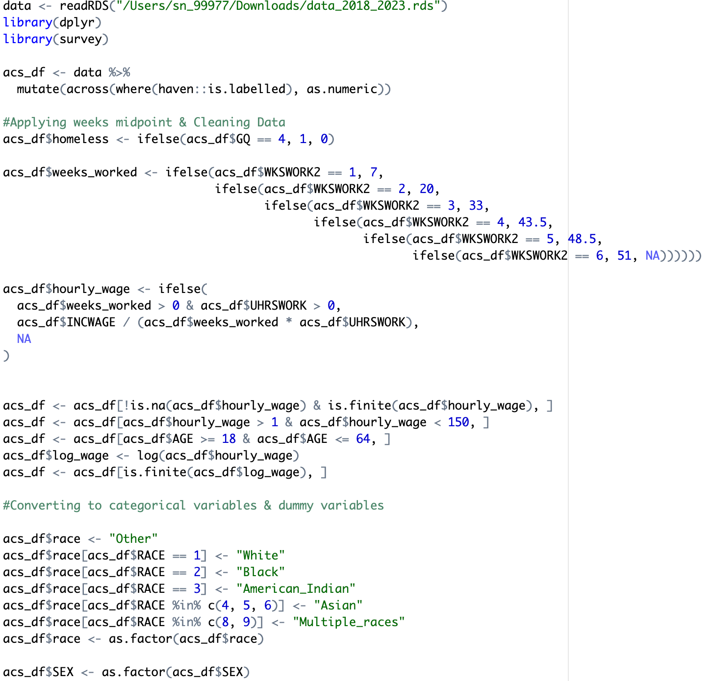
To get their hourly earnings, we translated the “WKSWORK2” variable using the category labels to create a midpoint for each numerical value to show the hours worked per person, transforming them from coded values into a series that contains the actual number of weeks worked called “weeks_worked”. Then we calculated the hourly wage with the “INCWAGE” and “UHRSWORK” variables, which are income and hours worked, respectively, per individual, by multiplying “weeks_worked” by “UHRSWORK”, and then dividing from “INCWAGE”. Threshold trimming was applied to the hourly wages in order to remove implausible values such as values less than $0 and values greater than$ 200. Any missing values in the original data were removed.

Considering that the “GQ” variable — which explains a person’s group quarters or living situation — shows sheltered homelessness, a new column was created to categorize people with different coded values. People with coded values of 4 were categorized under homelessness, denoted with the value 1, and people with “GQ” 1, 2, 3, and 5 were denoted with 0, showing stable housing.

New Variable	Variables Used	Recording
weeks_worked	WKSWORK2	Midpoints calculated with category labels
hourly_wage	INCWAGE, weeks_worked, UHRSWORK	INCAGE/ (weeks_worked * UHRSWORK)
adjusted_hourly_wages_2023	hourly_wage, YEAR, CPI	hourly_wage/CPI[YEAR]
homeless	GQ	If 4, GQ = 1; else GQ = 0
monthly_salary	UHRSWORK, weeks_worked, adjusted_hourly_wages_2023	(UHRSWORK * weeks_worked * adjusted_hourly_wages_2023)/12

Table 1 | A Recording Table showcasing all the computations for IPUMS variables.

Categorical variables such as race, education, sex, and age were also transformed into various factors in RStudio for upcoming survey-weighted regression analysis. Normalized weights were applied to hourly wages to maintain a simplified depiction of the weights onto the sample size without altering their importance on the data. The variables race and education were transformed into dummy variables, where each race and education level was split into different categories. Race was transformed into the variables “White,” “Black,” “American_Indian,” “Asian,” “Multiple_Races,” and “Other” with “White” as the reference; education was transformed into “No_schooling,” “Middle_school,” “High_school,” “College,” and “Missing,” using IPUMS category labels, with “High_school” as the reference. Similarly, the variable sex included male and female, in which male was made as a reference for female automatically. Age was split into “18-30,” “30-40,” “40-50,” “50-60,” and “60-64,” the reference being “60-64.”

Inflation Adjustments and Weighting

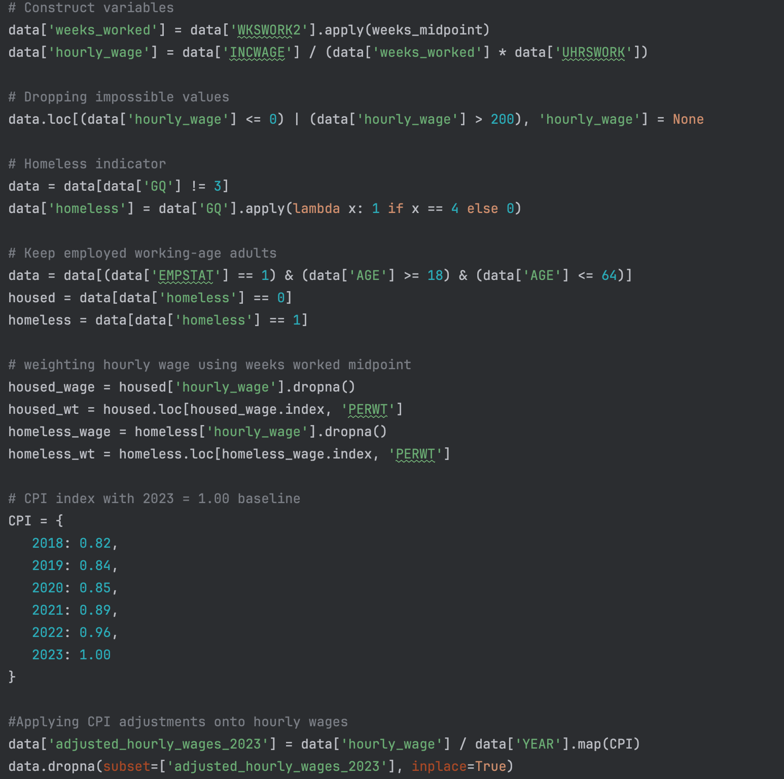
The next step in our process was to account for inflation in order to allow comparison between homeless and housed workers over the years. It would be incorrect to not include the influence of inflation on wages, especially after the impact of the COVID-19 pandemic during 2020 to 2021. From 2018, the change in inflation has been accelerating, ranging from 1.2% to 8.0%, which makes it ever more crucial to adjust the hourly wages in each year to become uniform with each other¹⁷. We normalized the data by taking the annual average CPIs per year from 2018 to 2022 and creating ratios in relation to 2023 as 1.00. Using 2023 dollars as a benchmark for the other years, we divided hourly wages with the wage ratios. Taking the annual average CPIs per year (2018 to 2023) from the Federal Bank of Minneapolis, we created approximate ratios, displayed in the table below.

YEAR	YEAR[CPI] : 2023[CPI]	Calculation
2018	0.82	251.1/304.7
2019	0.84	255.7/304.7
2020	0.85	258.8/304.7
2021	0.89	271/304.7
2022	0.96	292.7/304.7
2023	1	304.7/304.7

Table 2 | A CPI adjustment table using values from the Federal Bank of Minneapolis’s annual CPI report¹⁷.

The above values made wage calculations simpler by allowing the hourly wages in 2018 to 2022 to be divided by their factors, instead of using the complete CPI formula.

(1) $\begin{equation*}\text{YEAR 2 Price} = \text{YEAR 1 Price} \times \left(\frac{\text{YEAR 2 CPI}}{\text{YEAR 1 CPI}}\right)\end{equation*}$

The adjustments were inputted into the formula, and the changes were made to the hourly wages from 2018 to 2022, creating a uniform manner to compare hourly wages across years. The adjusted hourly wages were inputted into a series, or a one-dimensional column in our dataframe, labeled “adjusted_hourly_wages_2023.”

Along with inflation adjustments, the data was again standardized through the process of weighting the hourly wage per person. Weighting is a procedure that’s used to display the actual importance of each data point with relevance to the true population proportion in order to get accurate results from surveys. This procedure is extremely critical because it limits the influence of nonresponse bias, a bias that influences the data when survey participants do not respond to the survey at all or skip specific questions¹⁸. The effect of a nonresponse bias is grave, especially on probability-based surveys such as the American Community Survey, as they weaken inferences about a population from the sample survey data, which is why using sampling weights that the American Community Survey provides is crucial for producing accurate estimates of hourly wages between housed and homeless workers¹⁹^,¹⁸.

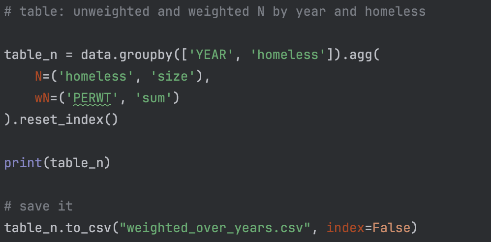
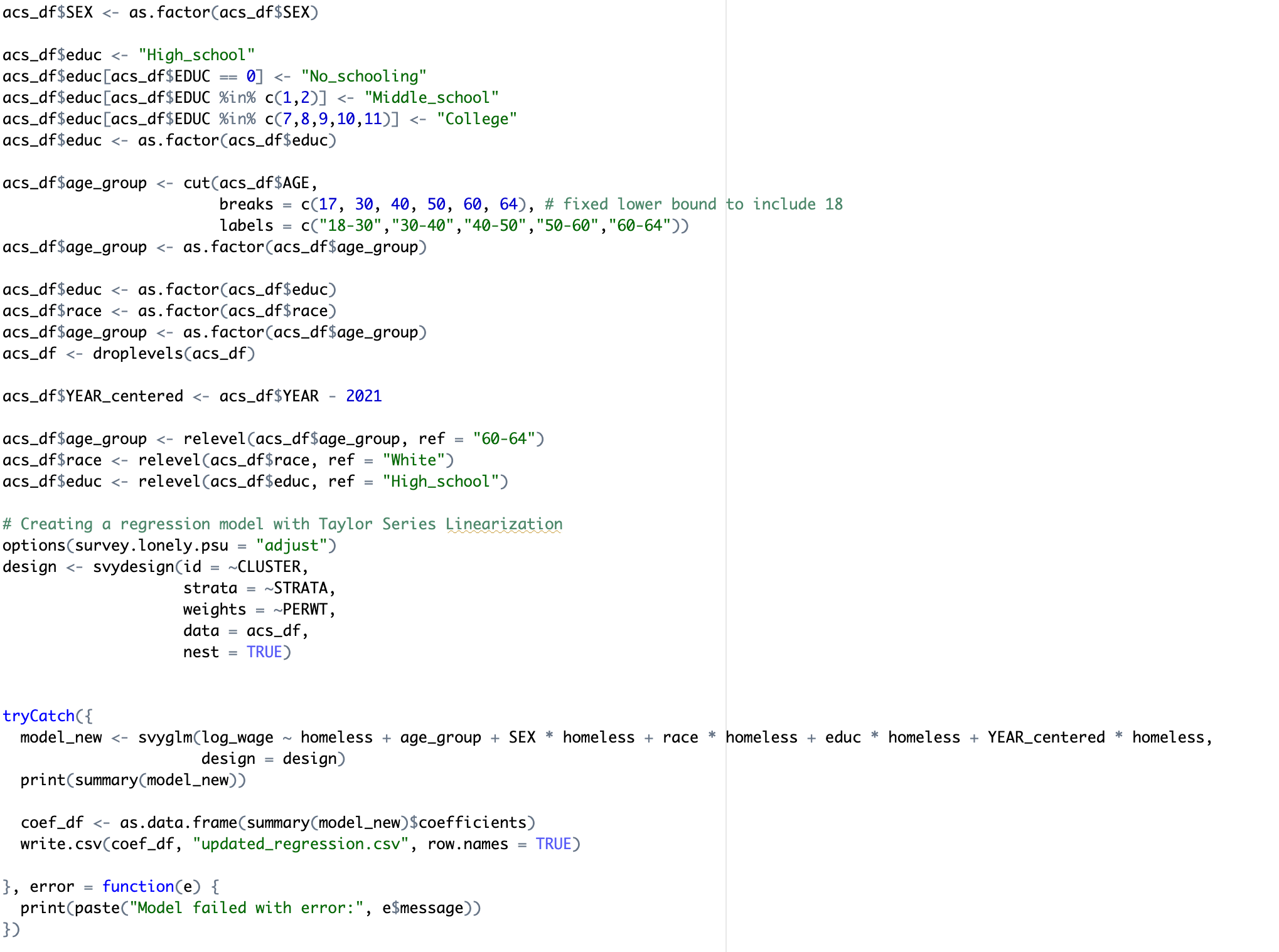
The American Community Survey data provides us with the variable “PERWT,” which was used to compute weighted median hourly wages accordingly to minimize sampling bias without multiplying hourly wages by PERWT weights. The upcoming statistical procedures such as the interaction tests and regression model are based on the weighted median hourly wages as a statistic, and their purpose is to take into account the American Community Survey design while testing for a statistical significance between subgroups and homeless hourly wages and overall between housed and homeless hourly wages. To capture the American Community Survey’s complex design, which includes strata and clusters, we implemented a Taylor Series Linearization on the data to compute weighted medians that don’t overlook these crucial factors, along with using PERWT weights. The PERWT weights produce medians that contribute to the distribution in proportion to their weights, and the Taylor Series Linearization estimates standard errors for hourly wages by including stratification and clustering in the American Community Survey’s survey. Through RStudio, the function svyquantile was used to calculate medians and standard errors through inverted confidence intervals. Failure to use such methods would ultimately produce biased estimates, especially when dealing with large skewed distributions. Hence, we produced weighted data that contains the adjusted influence of each data point without altering the actual variable (hourly wage).

Year	homeless	Unweighted n	Weighted n
2018	0	1275371	137395632.0
2018	1	26342	1512265.0
2019	0	1285479	138591473.0
2019	1	26335	1541861.0
2020	0	988159	133199029.0
2020	1	30500	1455981.0
2021	0	1229916	135631101.0
2021	1	26321	1456959.0
2022	0	1303060	140795544.0
2022	1	33046	1645303.0
2023	0	1318285	141731999.0
2023	1	32597	1659645.0

Table 3 | A comparison of weighted vs. unweighted sample sizes for each year.

After conducting the weighted procedures in order to display a representation of the actual population, we created a comparison of the unweighted sample size to the weighted sample size to show the effect weighting truly has.

Hourly Wage Sensitivity Analysis

In order to test the influence of the changes in the “WKSWORK2” variable instead of only using midpoints of its numerical values, we conducted a sensitivity analysis with lower bounds and upper bounds of each value. Using the numerical computations of the category labels shown in Table 3, we ran a sensitivity analysis using the lower bounds, midpoints, and upper bounds for all values of “WKSWORK2.” The values were recorded in the table below.

Year	Homeless Lower bound	Homeless Midpoint	Homeless Upper bound	Housed Lower bound	Housed Midpoint	Housed Upper bound
2018	$10.20 (0.613)	$10.10 (0.501)	$9.38 (0.913)	$24.39 (0.311)	$23.91 (0.305)	$22.70 (0.398)
2019	$12.5 (0.801)	$11.20 (0.677)	$9.16 (1.299)	$24.76 (0.467)	$23.34 (0.297)	$22.89 (0.292)
2020	12.55 (1.428)	$12.78 (0.943)	$11.31 (0.664)	$26.82 (0.458)	$25.63 (0.343)	$23.98 (0.490)
2021	$13.48 (1.375)	$12.48 (1.061)	$9.51 (0.986)	$25.69 (0.375)	$24.79 (0.285)	$24.31 (0.344)
2022	$11.59 (0.765)	$11.23 (0.943)	$10.02 (0.548)	$25 (0.384)	$24.51 (0.355)	$22.54 (0.281)
2023	$13.33 (0.744)	$11.45 (0.611)	$9.62 (0.576)	$25 (0.255)	$24.51 (0.250)	$24.04 (0.283)

Table 4 | Recordings of the median hourly wage for homeless and housed workers from the sensitivity analysis of variable “WKSWORK2”, with standard errors from the Taylor Series Linearization in parentheses.

From Table 4, we can analyze that the weighted median hourly wages for housed workers remain robust. The difference for the median hourly wage for housed workers is approximately a $2-3 difference, which suggests that the housed wages are not as sensitive to the weeks worked variable as homeless hourly wages are, which have a difference of about $3-4 from their lower bound, midpoint, and upper bound median hourly wages. While the homeless hourly wages are more sensitive to changes in the alternative values for the weeks worked variable, ultimately the greater overall trend of homeless workers having lower hourly wages than housed workers is shown. This shows that a wage gap is quite robust, but the magnitude of the wage gap remains sensitive due to the assumptions about the weeks worked.

While the results from the sensitivity analyses are subject to noise from other groups within the GQ code 4 that may affect the results of the median hourly wage, it’s also important to note the effects of the American Community Survey’s top-coding practices. Within many variables, the American Community Survey top codes variables to create a cap on extremely high values in order to mitigate the influence of outliers or skewness — one of them being the variable “INCWAGE.” However, the top-coding that the Census Bureau manages within the American Community Survey for age, tax, utility, and income data changes the value by only 0.1% off its original value, which reflects little to no effect on the income values collected through the survey²⁰. Now, the American Community Survey top-codes values for income that are at the 99.5th percentile per state, which compresses higher- income individuals, possibly understating the true wage gap that exists between housed and homeless workers²¹.

The income data collected by the American Community Survey is also vulnerable to self-reporting errors that heavily influence the measurement of hourly wage. For variables such as “WKSWORK2,” or the number of weeks worked per individual, the self-reporting error could affect the magnitude of the wage gap since alternative weeks worked affect the hourly wages, while the overall trend still remains robust.

Data Visualization

Year	Housing Status	Weighted Median Hourly Wage	Standard errors
2018	Housed	$23.91	0.304945994842571
2018	Homeless	$10.99	0.50170032210106
2019	Housed	$23.34	0.297685610256528
2019	Homeless	$11.20	0.677210955313317
2020	Housed	$25.63	0.34318678448102
2020	Homeless	$12.78	0.942547138324843
2021	Housed	$24.79	0.28525214656739
2021	Homeless	$12.48	1.06161614815879
2022	Housed	$24.51	0.355192710641067
2022	Homeless	$11.23	0.942672831246385
2023	Housed	$24.51	0.250056608326649
2023	Homeless	$11.45	0.611178311838145

Table 5 | A summary table consisting of weighted median hourly wages for years 2018-2023 for housed and homeless workers.

Table 5 demonstrates how the median hourly wage fluctuates between housed and homeless workers. The range of the median homeless worker hourly wage remains between $10 to $12, while the median housed worker hourly wage remains between $23 to $25.

Housing Status	Median Monthly Salary	Standard Errors
Housed	$3968.25	25.925
Homeless	$708.33	50.040

Table 6 | A Weighted Median Monthly Salary table by housing status in the years 2018 to 2023.

After calculating a weighted median monthly salary for both groups, a difference of approximately $3,260 was calculated between the housed monthly salary and the homeless monthly salary. While a large difference in wages is observed here, it is not appropriate to assume it’s statistically significant without testing for it.

Survey-Weighted Regression Model

For this study, a survey-weighted regression model for identifying potential wage differences is the most appropriate model because the relationship between confounding variables and wage for housed and homeless people is not homoscedastic²². Therefore, a homoscedastic regression model without weights would overlook group differences that a survey-weighted regression would take into account, while simultaneously using sampling weights and the strata and clusters from the American Community Survey data. Before starting the regression model, the significance level was set to α= 0.05, and the hypotheses are as follows:

(2) $\begin{equation*}H_0: \beta_1 \cdot \text{homeless} = 0\end{equation*}$

(3) $\begin{equation*}H_a: \beta_1 \cdot \text{homeless} \neq 0\end{equation*}$

Through RStudio, a survey-weighted regression model that includes several interaction tests and accounts for the variables housing status, age, sex, race, and education was run. Along with PERWT weights, the function svyglm() was applied to include strata and clusters through Taylor Series Linearization. Because homelessness interactions were included in the regression model and housed individuals served as the reference housing category, the main effect coefficients for these covariates were interpreted relative to housed individuals as well as their individual references.

The variables race and education were transformed into dummy variables, where each race and education level was split into different categories. Race was transformed into the variables “White,” “Black,” “American_Indian,” “Asian,” “Multiple_Races,” and “Other,” according to the provided IPUMS category labels, with the reference being the race “White” as it is the most prevalent in the data. Education was also transformed into “No_schooling,” “Middle_school,” “High_school,” “College,” and “Missing,” using IPUMS category labels, with the reference “High_school” to allow for comparison to a middle baseline. Similarly, the variable sex included male and female, in which male was made as a reference for female automatically. The variable year was kept as a continuous variable rather than a categorical variable to test the average yearly rate of change in hourly wages, and it was centered around 2021 to avoid R beginning the regression model at year 0 A.D. It’s important to clarify to R that year 0 means 2021 instead of 0 A.D., which is a misunderstanding that can produce extremely incorrect coefficients. YEAR was centered around 2021 such that 2018–2023 were coded as -3, -2, -1, 0, 1, and 2, respectively. Year centering is also simply a process that uses the entire scope of the data to produce accurate coefficients in reference to the centered year, reducing multicollinearity and avoiding mistakes that R would automatically make with the variable YEAR.

However, for age, we demonstrated how wages don’t decrease smoothly with an increase in age, but instead, they decline when an individual approaches their retirement stage due to a drop in hours worked and transition from full-time to part-time work. This method disproves the traditional economic theory of wages behaving in an inverted U-shape, where individuals experience a smooth drop in wages with a rise in age, as it is believed that wage and income peak and drop over the age of 55²³. Several studies have shown that they tend to drop when an individual nears a retirement or a partial retirement stage, showing that not all wages decline with a certain age²⁴.

We applied a “step method,” which transforms age into a categorical variable with multiple intervals to show how wage changes with varying ages. Age was split into “18-30,” “30-40,” “40-50,” “50-60,” and “60-64,” with age “60-64” as the reference to allow for easier comparison between wages for younger people, who don’t approach a near-retirement stage. Finally, to handle large sets of skewed data, log wage was applied to reduce the heteroskedasticity and to provide percent-based interpretations using American Community Survey data and weights. Using the function svyglm() in RStudio automatically creates references for each categorical variable, which, in this case, created the references ages 60-64 for age_group, the race “White” for race, and “High_school” for education. The reference level was adjusted to fit the desired level rather than just the first one.

Along with regression to take into account confounding variables, several interaction tests between variables were included to analyze any differences and trends over years. Three interaction tests have been included with the variable homeless to show association among homeless and race, education, and sex individually. A homeless and year interaction test was also included in the regression to highlight any year to year variance along with homeless hourly wages to identify any association between hourly wages across different years. The formula below represents the survey weighted regression relationship.

(4) $\begin{equation*}\footnotesize\begin{split}\log(\text{wage}) \sim{} & \beta_0 + \beta_1 \cdot \text{homeless} + \beta_2 \cdot \text{age\_group} + \beta_3 \cdot (\text{sex} \cdot \text{homeless}) \\& + \beta_4 \cdot (\text{race} \cdot \text{homeless}) + \beta_5 \cdot (\text{education} \cdot \text{homeless}) \\& + \beta_6 \cdot \text{YEAR} + \beta_7 \cdot (\text{YEAR} \cdot \text{homeless})\end{split}\end{equation*}$

Results

Figure 1 | A computer output table of the survey-weighted regression model.

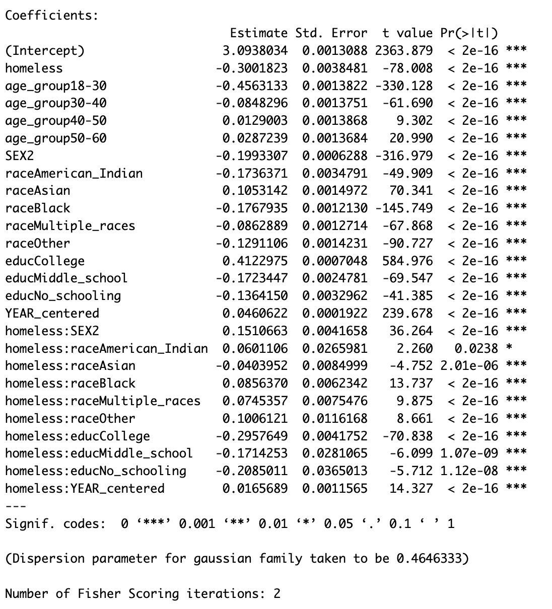
Percent Change = (e^β – 1) x 100

The results of the survey-weighted regression model are shown above, and using the formula to interpret the coefficients, it can be seen that approximately homeless individuals in the reference categories earn 26% lower wages than housed individuals do after holding all other factors constant. Gender differences also show that housed females (SEX2) earn roughly 18% lower wages than housed men do when holding all factors constant. Education coefficients for housed individuals demonstrate that college graduates earn 50% higher wages, middle school graduates earn 16% lower wages, and no schooling individuals earn 12% lower wages than high school graduates, when holding all other factors constant. Compared to the reference category of white housed individuals, Black housed individuals earn roughly 16% lower wages, American Indian housed individuals earn 16% lower wages, housed individuals of multiple races earn 8% lower wages, housed individuals of other races earn 12% lower wages, and Asian housed individuals earn 11% higher wages, when holding all factors constant. The variable ages show that for housed individuals, 18-30 year olds earn 36% lower wages than individuals ages 60-64, while individuals ages 30-40 earn 7% lower wages, individuals 40-50 earn 1% higher wages, and 50-60 year olds earn approximately 3% higher wages than people 60-64, when holding all other factors constant. Finally, since year was added as a continuous variable, we can infer that there is a 4.6% average annual increase in hourly wages for all housed individuals when all other factors are constant.

The interaction between homelessness and sex demonstrated that females experiencing homelessness earn approximately 14% lower hourly wages than housed females, compared to approximately 26% lower hourly wages among males in the reference category, indicating a weaker negative association between homelessness and hourly wage among females. Similarly, among the interaction tests for education and homeless, the model displays that college-educated homeless individuals earn approximately 45% lower hourly wages, homeless individuals with middle school education earn approximately 38% lower hourly wages, and homeless individuals with no schooling earn approximately 40% lower hourly wages than homeless individuals with high school education, highlighting the high degree of variation among homeless individuals and hourly wages across the different education levels. The interaction test between race and homeless demonstrates that Black homeless individuals earn approximately 19% lower hourly wages, American Indian homeless individuals earn approximately 21% lower hourly wages, homeless individuals of multiple races earn approximately 20% lower hourly wages, individuals of other races earn approximately 18% lower hourly wages, and Asian homeless individuals earn approximately 28% lower hourly wages, when compared to homeless White individuals. Looking at the YEAR and homeless interaction, the average annual increase in hourly wages is approximately 6.2% for homeless individuals which is higher than the average annual rate of change in hourly wages of 4.6% for housed individuals.

Survey-weighted Interaction testing displayed statistically significant analyses with p-values < α= 0.05, demonstrating that homeless hourly wages vary between different subgroups and over years. Testing showed variation among different races, educational groups, and sexes, while displaying a change in hourly wages over 2018-2023. This regression model displays p-values < α= 0.05, suggesting that the covariates age group, sex, race, and education are statistically significant, and they play a role in influencing the variation in log hourly wages. Since the p-value < 2e-16 for the predictor homeless is below α= 0.05, we can reject H₀. There is statistical evidence that homelessness is associated with lower hourly wages. The coefficient of -0.300 indicates that the predictor homelessness is negatively associated with hourly wages after controlling for covariates.

Discussion

The finding of a 26% wage disparity from the study aligns with existing studies that highlight the income disparity between homeless and housed employees.

Since our data is collected from a survey run by the American Community Survey, the data that workers report is subject to a self-response bias: a natural tendency to report false or inaccurate information. The self-response bias includes social desirability bias, extreme response bias, and acquiescence. Social desirability bias leads people to input answers they believe will present themselves in a favorable light, aligning with social standards and avoiding judgment from the interviewers; extreme response bias is the tendency to select extreme options within a rating scale in a survey; acquiescence is the tendency to pick the choice “agree” to questions²⁵. Although all three biases play a role in a survey, the most prevalent is the social desirability bias in the American Community Surveys. Across various topics in the American Community Survey and the variables collected for the study, the most prone to the social desirability bias include criminal behavior, education, and economic information, where participants may misreport or deny certain behaviors²⁶. In this case, several factors are subject to such biases, but the biases are not limited to only these variables. These types of biases can lead to measurement errors and data distortion, which limit the ability to generalize the findings to the population due to inaccurate assessments.

The “GQ” variable also limits generalizability because the analysis is based on sheltered homeless individuals and may not represent all homeless or housed populations. Since we exclude unsheltered homelessness, the estimate may not be a generalizable statistic, as more vulnerable populations have not been included in the process. As a result, the observed difference in median wages may not extend to broader populations beyond the study sample. This may potentially cause our results to underestimate the true wage gap that exists because of the absence of more economically vulnerable individuals in the data.

Additionally, American Community Survey top-coding practices may not have an extreme influence on the data, but compressing higher-income individuals may underestimate the true wage disparity of 26% fewer hourly wages for homeless individuals. This shows to be a possible limitation to be considered in analysis when applying the statistic of 26% fewer hourly wages.

The findings of this study should not be used to prove that low wages cause homelessness, but rather that wage differences contain a link to housing status, which should be considered in future policies. The study only depicts an association between homeless workers and hourly wages but does not hope to show causation between the two.

Conclusion

In this study, we analyzed the survey data collected from the American Community Survey to understand if homeless workers get paid less than housed workers. We cleaned the data to remove unsuitable individuals and incorrect values and adjusted the data accordingly, finding that homeless workers do get paid less than their housed colleagues. The median housed worker hourly wage is approximately between $25 and $27, while the median homeless worker hourly wage is approximately $10 to $12. Several interaction tests between the variable homeless and demographic subgroups showed that hourly wages for homeless people differ across races, education levels, and sex. The survey-weighted regression model also revealed a statistically significant percent difference of 26% in hourly wages between homeless and housed individuals, with homeless workers earning 26% less hourly wage than housed workers.

Referring back to the Labor Economics framework, we can connect our findings of a 26% wage disparity between housed and homeless workers as a result of labor market segmentation. A primary sector and secondary sector form from a division made by outside forces and standards, restricting upward mobility and limiting economic growth for homeless individuals, especially when a 26% wage disparity exists. Due to the primary sector consisting of high wages and stable jobs, the wage disparity proposes significant economic barriers for economic opportunity and mobility within the market. The visible disparity could potentially be a limitation to the growth in employment opportunities and job search as the division limits the access to the primary sector. The results link wages back as a barrier to economic growth that many homeless individuals experience, restricting them from gaining future opportunities as it keeps them within their own social status.

Appendix

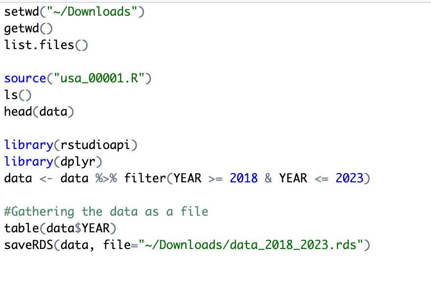
Appendix 1: RStudio code to convert the American Community Survey data into an RDS file.

Appendix 2: Python code for cleaning and weighting the RDS data.

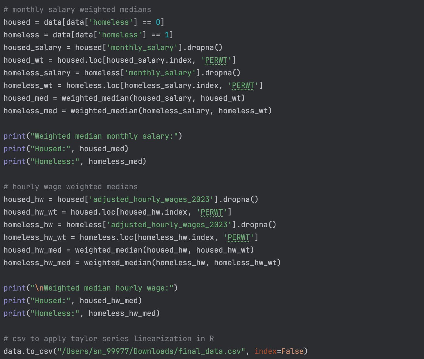
Appendix 3: RStudio code to apply Taylor Series Linearization with Python Data.

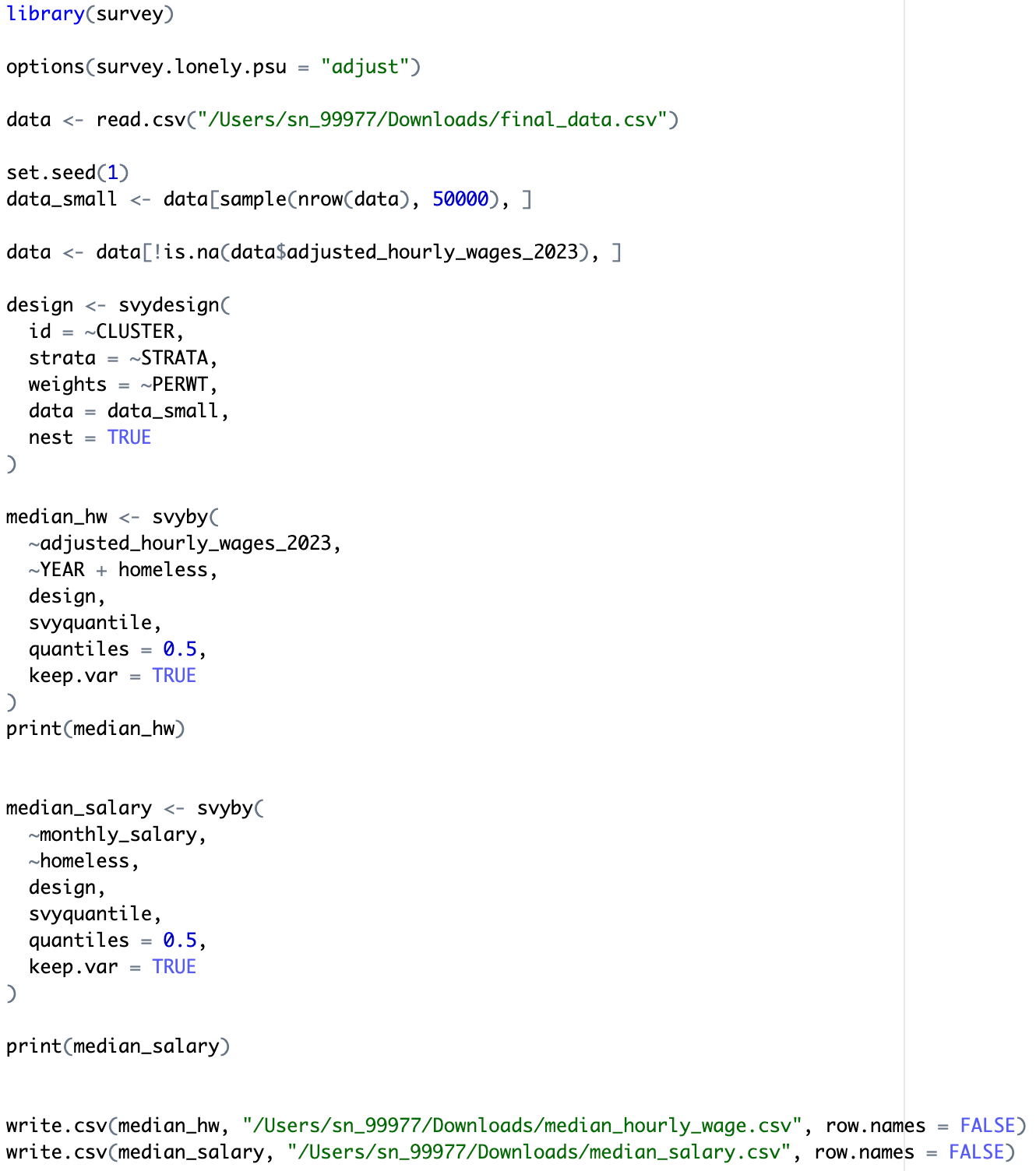
Appendix 4: Python code for a summary table for weighted median hourly wage by year.

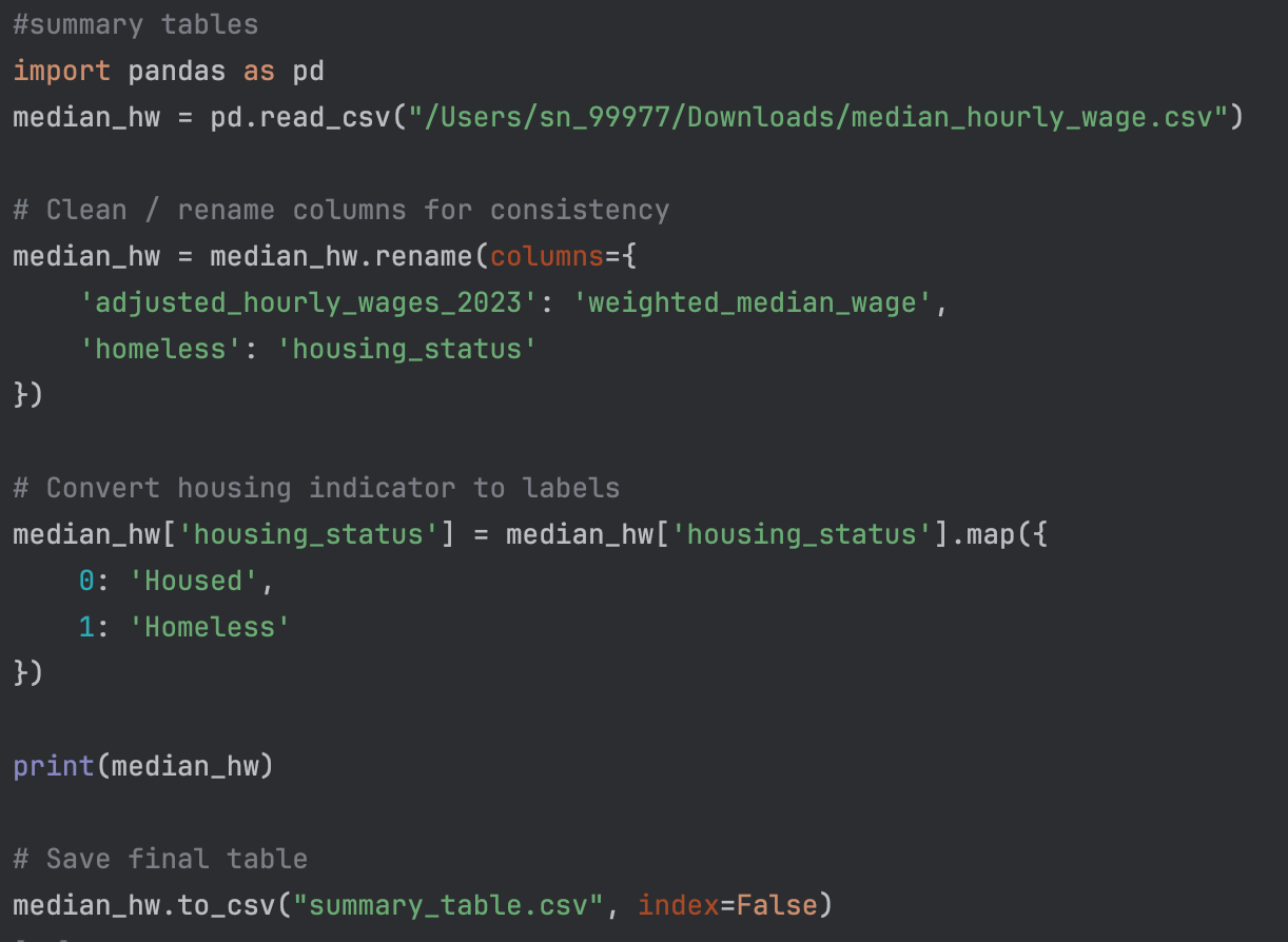
Appendix 5: Python code for a table of unweighted and weighted sample size by year.

Appendix 6: R Studio code to computing a survey-weighted regression model.

References

B. D. Meyer, A. Wyse, A. Grunwaldt, C. Medalia, D. Wu. Learning about Homelessness Using Linked Survey and Administrative Data. NBER Working Paper 28861, 2021, https://doi.org/10.3386/w28861. [↩]
M. Henry, T. de Sousa, C. Roddey, S. Gayen, T. J. Bednar. The 2020 Annual Homeless Assessment Report (AHAR) to Congress. The U.S. Department of Housing and Urban Development, 2020, https://www.huduser.gov/portal/sites/default/files/pdf/2020-ahar-part-1.pdf. [↩]
T. de Sousa, A. Andrichik, E. Prestera, K. Rush, C. Tano, M. Wheeler. The 2023 Annual Homelessness Assessment Report (AHAR) to Congress. The U.S. Department of Housing and Urban Development, 2023, https://www.huduser.gov/portal/sites/default/files/pdf/2023-AHAR-part-1.pdf. [↩]
Codebook for an IPUMS USA Data Extract. IPUMS USA. https://live.usa.datadownload.ipums.org/web/extracts/usa/2736066/usa_00001.xml?jwt=eyJhbGciOiJSUzI1NiJ9.eyJpc3MiOiJ1bWEiLCJleHAiOjE3NzkzMjk1NDgsIm5iZiI6MTc3OTMyODY0OCwic3ViIjoiMTM4OGFjNDAtYzA1Ni0wMTNlLWZiMWMtMDI0MjBhMWMwMzA0IiwiY29sbGVjdGlvbnMiOlsidXNhIl19.YxPu-uB1Kn9IbvZho9Oz_Wa1vPtkXX_BtlV2sx4yPaKidb0ATBWbR9NXNkkWd98FN2kCbg1y0LAAckPRWRVI6Gpw8DImr23rxn5LcxxNOLdBhvIgu01zerHwhoWpb81ZjVQeLz6oZB0hG5663-mCvBukNzmA7jNdO-VCDDVY_FVo0xqAt1fdxHF-0jTeJ88_k4g6unfl6blnmZ57y5Lwq-vwO4cbng-lEOUTZOPMyyoBTxaYiWoUOYr2kg-RE19z1eFjReoo2WC8mplI4G010L4Cap2vu3MRdlFY9Hn6ww6ZHu2BzU8WBq0tgepw4vPuevtJEfYn8kItlhfg9qO3XQ#fileDscr. [↩]
S. Ruggles, S. Flood, M. Sobek, D. Backman, G. Cooper, J. A. R. Drew, S. Richards, R. Rodgers, J. Schroeder, K. C. W. Williams. IPUMS USA: Version 16.0 [dataset]. Minneapolis, MN: IPUMS, 2025, https://doi.org/10.18128/D010.V16.0 . [↩]
H.N. Butler. Economic Analysis of Labor Markets: A Framework for Analyzing Employment Law Issues. Kansas Journal of Law & Public Policy. Vol. 8, pg. 1–21, 1998, https://ssrn.com/abstract=6759578. [↩]
M. Reich, D. M. Gordon, R. C Edwards. Dual Labor Markets: A Theory of Labor Market Segmentation. American Economic Review. Vol. 63, pg359-365, 1973, https://digitalcommons.unl.edu/cgi/viewcontent.cgi?article=1002&context=econfacpub. [↩]
W. T. Dickens, K. Lang. Labor Market Segmentation Theory: Reconsidering the Evidence. NBER Working Paper 4087, 1992, https://doi.org/10.3386/w4087. [↩]
S. Golabek-Goldman. Ban the Address: Combating Employment Discrimination Against the Homeless. The Yale Law Journal. Vol. 126, pg. 1789-1868, 2017, https://yalelawjournal.org/note/ban-the-address-combating-employment-discrimination-against-the-homeless. [↩]
D. Poremski, J. Woodhall-Melnik, A. J. Lemieux, V. Stergiopoulos. Persisting Barriers to Employment for Recently Housed Adults with Mental Illness Who Were Homeless. Journal of Urban Health. Vol. 93, pg. 96-108, 2017, https://doi.org/10.1007/s11524-015-0012-y. [↩]
IPUMS USA: Descr: GQ. IPUMS USA, 2024, usa.ipums.org/usa-action/variables/GQ#comparability_section. [↩]
Category 1: Literally Homeless. HUD Exchange, 2025, www.hudexchange.info/homelessness-assistance/coc-esg-virtual-binders/coc-esg-homeless-eligibility/four-categories/category-1/. [↩]
2022 American Community Survey/Puerto Rico Community Survey Group Quarters Definitions. United States Census Bureau, 2022, https://www2.census.gov/programs-surveys/acs/tech_docs/group_definitions/2022GQ_Definitions.pdf. [↩] [↩]
P. R. Voss, K. Marton. Small Populations, Large Effects: Improving the Measurement of the Group Quarters Population in the American Community Survey. National Academies, 2012, https://doi.org/10.17226/13387. [↩]
Sample Design and Estimation in the American Community Survey (ACS) and the Puerto Rico Community Survey (PRCS). IPUMS USA, 2025, usa.ipums.org/usa/voliii/ACSsamp.shtml. [↩]
S. G. Vidal, E. Jensen, J. Eggleston, E. Castro. Understanding the 2024 American Community Survey 1-Year Estimates. United States Census Bureau, 2025, www.census.gov/newsroom/blogs/random-samplings/2025/09/acs-1-year-estimates.html. [↩]
Consumer Price Index, 1913- | Federal Reserve Bank of Minneapolis. Federal Reserve Bank of Minneapolis, 2023, www.minneapolisfed.org/about-us/monetary-policy/inflation-calculator/consumer-price-index-1913-. [↩] [↩]
A. Koch, M. Bloom. Nonresponse bias. GESIS – Leibniz Institute for the Social Sciences, 2016, https://doi.org/10.15465/gesis-sg_en_004. [↩] [↩]
National Research Council. Nonresponse in Social Science Surveys: A Research Agenda. The National Academies, 2013, https://doi.org/10.17226/18293 [↩]
IPUMS USA | Top and Bottom Codes. IPUMS USA, 2016, usa.ipums.org/usa/volii/top_bottom_codes.shtml. [↩]
IPUMS USA: Descr: INCWAGE. IPUMS USA, 2024, usa.ipums.org/usa-action/variables/INCWAGE#codes_section. [↩]
W. H. DuMouchel, G. J. Duncan. Using Sample Survey Weights in Multiple Regression Analyses of Stratified Samples. Journal of the American Statistical Association. Vol 78, pg. 535-543, 2012, https://doi.org/10.2307/2288115. [↩]
R. Rich, J. Tracy, E. Fu. U.S. Real Wage Growth: Fast Out of the Starting Blocks. Federal Reserve Bank of New York, 2016, https://libertystreeteconomics.newyorkfed.org/2016/09/us-real-wage-growth-fast-out-of-the-starting-blocks/. [↩]
P. Rupert, G. Zanella. Revisiting wage, earnings, and hours profiles. Journal of Monetary Economics. Vol 72, pg. 114-130, 2015, https://doi.org/10.1016/j.jmoneco.2015.02.001. [↩]
K. Bognder, U. Landrock. Response Biases in Standardised Surveys. GESIS – Leibniz Institute for the Social Sciences, 2016, https://doi.org/10.15465/gesis-sg_en_016. [↩]
L. Burstzyn, I. K. Haaland, N. Röver, C. Roth. The Social Desirability Atlas. NBER Working Paper 33920, 2025, https://doi.org/10.3386/w33920. [↩]