NHSJS Reports

The Effect of Natural Error and Eavesdropping on the Performance of the BB84 Quantum Key Distribution Protocol

August 14, 2026

Abstract

Due to the advent of quantum computing, traditional encryption methods will be rendered vulnerable. To combat this risk, quantum key distribution protocols were developed. The Bennett-Brassard-84 (BB84) protocol is a quantum key distribution protocol designed to securely communicate one-time keys between two parties. One-time keys are a series of binary digits used to encrypt a message between two parties. In the BB84 protocol, a potential eavesdropper intercepting the communication or the natural error of the transmission system can both affect its performance. Although the relation between the quantum bit error rate and performance is known, finding a relation between error sources and error rate is vital. To better understand the relationship between error and performance and provide a framework for simulating QKD protocols, eavesdropper attack strength and natural system error were varied in a MATLAB simulation utilizing the BB84 protocol to analyze their effect on various performance metrics: Sifted Key Fraction (SKF), Quantum Bit Error Rate (QBER), and Secure Key Rate (SKR). By using simulations of individual BB84 protocol applications, the results show that the quantitative relation between the QBER and the error sources is bilinear and is given by $QBER=(1-\frac{s}{2})p+\frac{s}{4}$ , where s and p are the eavesdropper attack strength and bit-flip probability respectively. The simulations also demonstrate finite-key effects near the maximum tolerable QBER boundary for the SKR.

Keywords: Quantum key distribution, BB84, quantum cryptography.

Introduction

Secure communication is vital for maintaining the integrity and authenticity of sensitive information. Cryptography, the science of disguising messages to increase their security, has been implemented in computer systems and communications to achieve this¹. Algorithms such as the Rivest-Shamir-Adleman (RSA) algorithm have relied on the time complexity of factoring large numbers to prevent decryption². With the invention of quantum computers capable of exponentially more computing power than classical ones, standard encryption algorithms relying on time complexity as a barrier to decryption were made vulnerable. The invention of Quantum Key Distribution (QKD) protocols was driven by a need for new methods that couldn’t be broken by quantum computing. QKD protocols work through the inviolability of the laws of physics, laws which cannot be broken by quantum computers. Unlike modern algorithms such as RSA which rely on time complexity to prevent decryption, the principles of QKD protocols provide higher security against quantum computers. Such QKD protocols are the Bennett-Brassard 1984 Protocol (BB84 Protocol) and Ekert 1991 Protocol³. The first QKD protocol was the BB84 protocol, proposed by Charles Bennett and Gilles Brassard in 1984, a popular protocol that has been used in applications such as the SwissQuantum QKD Network⁴.

Key Exchange

Before discussing QKD, it is vital to first understand the mechanisms of data and protocol key transfer. A general one-time key encryption/decryption protocol works by both the sender and receiver first having a copy of the private one-time key that they have securely communicated with each other. In a message, words can be split into their individual letters. The letters may then be represented in binary. In this manner, the whole message can be changed to binary. Then, the encrypted message is formed through addition of the message with the key through the XOR operation. After adding the key to the message, the sender gives this new sequence to the recipient through an open channel. The message can be sent in an open channel because anyone who intercepts the message will be unable to decipher it, as without the one-time key, the message is a random cluster of 1’s and 0’s. After receiving the message, the receiver applies the XOR operation with the key and the encoded message they received to obtain the original message⁵. The problem lies in securely sending the key that both parties use. This is where QKD protocols come in, as they can securely generate and communicate random one-time keys. In sending these keys, if the error rate is too high, there is a probability that an eavesdropper is present, and the key can simply be thrown away.

BB84 Protocol

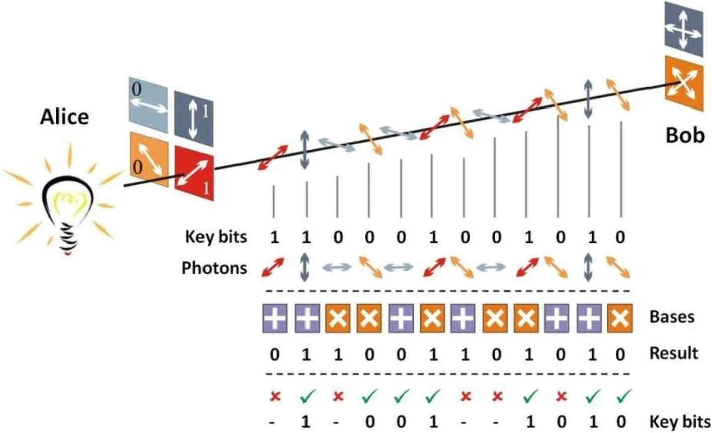
The BB84 protocol works between two communicators, Alice (sender) and Bob (receiver). If Alice wants to send $n$ bits, then both Alice and Bob randomly generate a set of $n$ bases, either in the “+” (rectilinear) or “x” (diagonal) basis. Next, Alice generates $n$ random bits, either 0 or 1. In order to represent these bits, she uses photons, elementary particles of light. The specific property of these photons she uses is their polarization angle, the orientation of their electric fields oscillating. In the rectilinear basis, a polarization angle of 0 represents a 0, and an angle of $\frac{\pi}{2}$ represents a 1. In the diagonal basis, an angle of $\frac{\pi}{4}$ represents a 0, and an angle of $\frac{3\pi}{4}$ represents a 1⁷. Next, based on the bit and the basis Alice has randomly chosen, she sends Bob a photon with the chosen polarization. Bob, in his randomly chosen basis then measures the photon sent by Alice. If both Alice and Bob are using the same basis, then Bob will correctly measure the bit value of the photon Alice sent. However, if they are using different bases, then Bob will measure either bit in his chosen basis with equal probability. This is due to the superposition principle in quantum physics. The superposition principle is the principle that a quantum state can be represented as a linear combination of other quantum states. For the photon, a polarization of $\frac{\pi}{2}$ in the rectilinear basis, when measured in the diagonal basis, undertakes a superposition of the polarizations $\frac{\pi}{4}$ and $\frac{3\pi}{4}$ . 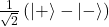The new state of the photon is $\frac{1}{\sqrt{2}}\left(|+\rangle - |-\rangle\right)$ .

Each state is represented with ket notation, where the probability for a certain state to be the result of a measurement is equal to its coefficient squared. In this case, the $\frac{1}{\sqrt{2}}$ coefficient arises from the fact that the probabilities of the superposition need to add to 1⁸. From adding the squares of the coefficients, the total probability is indeed $(1/\sqrt{2})^2+(1/\sqrt{2})^2=1/2+1/2=1$ . After Bob makes his measurement in the opposite basis, his measured bit has a 50% chance of being the same bit Alice sent. After all the bits are sent and received, Alice and Bob check with each other to see what bases they used. This can be done on an open channel, as it doesn’t reveal the bits themselves. After sharing, they discard all the bits in which they didn’t share a basis to ensure they are working with the same bits, a process called sifting. Then, they confirm the security of their key by checking some bits with each other, which they won’t be able to use in their key. After confirming the security of their bits, they use those bits to form a binary key which can be used to encrypt messages⁷.

If an eavesdropper is listening while the keys are being distributed, the key shouldn’t be used. The BB84 protocol has been proven to be information-theoretically secure against general attacks in the asymptotic limit of infinitely long keys, regardless of the computing power of the attacker⁹,¹⁰,¹¹,¹²,¹³, and is usable as long as the total Quantum Bit Error Rate (QBER) remains below approximately 11%, as demonstrated by Shor and Preskill (2000)¹¹. There are many types of attacks that an eavesdropper can utilize, such as intercept-resend, beam-splitting, photon-number splitting, trojan horse, unambiguous state discrimination, etc.¹³,¹⁴,¹⁵. This study deals specifically with the intercept-resend model of eavesdropping.

Theoretical Model

In this model, when an eavesdropper is intercepting the photons, they must take a measurement of the photon in a randomly chosen basis, either rectilinear or diagonal. Then, the eavesdropper sends out the bit they measured in their chosen basis to the original receiver, to appear as though no interference was there¹⁶. For the eavesdropper, ideally, they would clone the photon and measure the cloned photon to not interfere with the original, but according to the no-cloning theorem, this isn’t possible. The no-cloning theorem states that it isn’t possible to create an exact copy of an arbitrary quantum state¹⁷, so the eavesdropper must settle for measuring the original and retransmitting to the receiver. When the sender and receiver are using a certain basis, and the eavesdropper is using a different basis, errors in bit values can occur from the polarization of the photon not being aligned in all of the bases. The interference of the eavesdropper then causes errors in bit values which the sender and receiver can measure. Apart from errors induced by an eavesdropper, there are sources of error that result from the equipment used to facilitate the protocol.

In this paper, we adopt a simplified model in which ‘natural’ error is approximated to a bit-flip probability, $p$ . It should be noted although Shor and Preskill (2000) used separate bit-flip and phase-flip errors to bound error correction and privacy amplifications losses separately, we assume a symmetric depolarizing channel where $e_b≈e_p=p$ ¹¹. It should also be noted that although we consider an ideal BB84 protocol, real QKD systems are affected by many flaws, such as a basis-dependent source, nonrandom phase, and encoding flaws¹⁸. They can also be caused by transmission equipment imperfections such as polarization switching caused by a vertical-cavity surface-emitting laser (VCSEL)¹⁹, transmission losses from optical fiber or free space²⁰, or dark counts²¹. In addition, we assume ideal photon sources and perfect detectors.

Additionally, there are finite-key effects that are not assumed in much of the security analysis literature. In real implementations, there are a finite number of bits exchanged, meaning the asymptotic assumption is overestimating the true SKR²². In this paper, the QBER is simulated through a finite-key model but with the intention of approximating the asymptotic regime.

Recent studies have increasingly discussed the real-world imperfections and effects on the performance that quantum key distribution systems can bring. In simulation-based studies, specifically, Pereira et al. (2023) demonstrated the security of the BB84 protocol for source imperfections and attacks²³. For Monte Carlo approaches to QKD simulation, there has also been a general QKD security study by Su (2023) for calculating key rates and evaluating information-theoretic security²⁴. Dhakal et al. (2025) have simulated the BB84, E91, and EBB84 protocols when changing key-lengths, finding that there are security tradeoffs between them²⁵. In analyzing the effects of key-length, Bunandar et al. (2020) analyzed the finite-key effect with numerical methods, finding a dependency in the non-asymptotic region²⁶. As we are grounded in a finite number of keys through simulation, we are working within the finite-key region. However, because the finite-key assumption is used in finding the QBER directly rather than the SKR (which is instead calculated from the QBER), the asymptotic limit approximation can stand. Although, there are a few finite-key effects which will be explored. There have been multiple programs that simulate BB84, such as through Qiskit, Python, as well as proprietary tools for engineering applications such as by Gkouliaras et al. (2024), Saeed et al. (2022), and Adu-Kyere et al. (2022)²⁷,²⁸,²⁹. While many studies tackle security and frameworks for simulation, we wish to demonstrate the principle of simulating QKD while working under natural error combined with eavesdropping, and in turn derive equations for this simplified model of an intercept-resend eavesdropper.

Research Objectives

As QKD protocols become more used, it will be useful to know the limits of the BB84 protocol. This can be done by finding the dependence of the protocol’s performance on its error, both natural and malicious. We hypothesize that the QBER will increase linearly with $p$ for a fixed value of $s$ , while the slope and intercept are determined by $s$ . The error sources are approximated as a combination of eavesdropping and bit-flipping. MATLAB was utilized to simulate the BB84 protocol between two parties with an eavesdropper in the middle. By providing pseudocode and validating quantum cryptography principles through simulation, we would like to provide a framework for future simulation-based studies of quantum key distribution.

Methodology

Parameters

First, we define the variables which impact the performance of the BB84 protocol. The eavesdropper attack strength, $s$ , represents the probability with which the eavesdropper intercepts a particular photon. It ranges from 0 to 1 where, for example, a value of 0.7 for $s$ indicates a 70% chance that the eavesdropper intercepts a particular transmission. The bit-flip probability, $p$ , ranges from 0 to 0.15 and represents the probability that a certain bit flips polarization during transmission. For example, a value of 0.05 represents a 5% chance that a particular bit flips. Together, $p$ and $s$ represent the interference that the protocol can face. The range of $s$ was chosen to demonstrate all frequencies of attack that are possible. The range of $p$ was chosen to represent the point of no natural error up to the maximum error (without any eavesdropping) before the SKR becomes 0. Since the maximum QBER tolerable is 11%, or 0.11, the maximum $p$ value is set at 0.15 to provide a buffer.

Metrics

Let us introduce the three metrics we will be analyzing to determine performance. Sifting is the process where the sender and receiver share what bases they use and then discard the bits for which they did not use the same basis. The Sifted Key Fraction (SKF) is the fraction of bits that remain after the sifting process. SKF can go from 0 to 1, with a 0 meaning that none of the bits remain after sifting, and a 1 meaning that every bit remains after sifting. An SKF of 0.5 means 50% of the bits remain after sifting.

The Quantum Bit Error Rate (QBER) is defined as the number of incoherent bits (bits where there is a mismatch, e.g., Alice sent a 1, but Bob received a 0) divided by the total number of sifted bits. The QBER is an important metric, as it represents the amount of error the sender and receiver are facing, where the lower the QBER the better the performance of the protocol. For example, if the sender and receiver use 100 bits of the same basis to check the security of their key, and there are 15 bits which don’t match between the two, then there is $15/100 = 15\%$ QBER. A 0% QBER means perfect transmission without error in the data, while 100% QBER means that for every bit the sender sends, the receiver will have the opposite bit.

From first principles, after Alice sends a photon, there is a probability $p$ that the bit-value flips. Additionally, there is a probability $s$ that it is intercepted. Because only the photons in which Alice and Bob measure in the same basis remain after sifting, those are the photons which will be counted. The first possible case is that the bit-value flips, but Eve does not intercept. The second case is that the bit-value does not flip, Eve intercepts with the wrong basis, and then Bob measures the incorrect bit-value. The third case is that the bit flips, Eve intercepts with the right basis, and then transmits the incorrect bit to Bob. The fourth case is that the bit-flips, Eve intercepts with the wrong basis, and Bob measures the incorrect bit. Adding the probability of each case, the expected QBER is

p(1-s) + (1-p)(s)\left(\frac{1}{2}\right)\left(\frac{1}{2}\right) + (p)(s)\left(\frac{1}{2}\right) + (p)(s)\left(\frac{1}{2}\right)\left(\frac{1}{2}\right)

= p – ps + \frac{s}{4} – \frac{ps}{4} + \frac{ps}{2} + \frac{ps}{4}

= p + \frac{s}{4} – \frac{ps}{2}

Thus, the expected QBER is $\text{QBER} = p + \frac{s}{4} - \frac{ps}{2} = \left(1 - \frac{s}{2}\right) p + \frac{s}{4}.$

The Secure Key Rate (SKR) demonstrates the efficiency of the protocol. Here, we define the SKR as the fraction of sifted bits that can be used in the key after error correction and privacy amplification are performed, rather than the standard rate of information transfer. The SKR is calculated based on the QBER, being found as

\text{SKR} = \text{Max}\big(0,\, 1 – f \cdot H(\text{QBER}) – H(\text{QBER})\big),

where f is the efficiency of the error correction algorithm and H(QBER) is the Shannon entropy function for a binary variable³⁰, calculated as

H(\text{QBER}) = -\text{QBER} \log_2(\text{QBER}) – (1-\text{QBER}) \log_2(1-\text{QBER})

Note that ‘Max’ indicates taking the highest value between the two inputs. An SKR of 1 would mean every single bit sifted would be able to be used in the key, while an SKR of 0 would mean none were usable. For an SKR of 0.20, 20% of sifted bits would be usable as part of the key³¹. In this paper, $f = 1$ is used. This corresponds to the Shannon limit of error correction as an idealized maximum³⁰. The effects of a changing $f$ will also be analyzed. For a typical error correction algorithm such as Cascade, the efficiency can range between 1 and 1.5³².

Simulation

In this paper, the BB84 protocol between a sender, a receiver, and an eavesdropper was simulated using MATLAB software. This study used simulations of 1000 bits, averaging 1000 trials for each data point, independently varying $s$ from 0 to 1 with 100 steps, and $p$ from 0 to 0.15 with 100 steps. A simulation of 1000 bits with 1000 trials per $(s,p)$ pair allows for a balance of accuracy and computational time. It will yield around 500 sifted bits, which is enough to reliably calculate the QBER. Additionally, for the number of trials, a similar logic was followed for optimizing the accuracy versus the computational time required. There are indeed finite-key limitations, but the number of bits and trials are attempting to minimize these limitations. QBER is measured directly from the finite simulation, but SKR is then calculated from that QBER using the asymptotic formula. The step sizes of 0.01 and 0.0015 were chosen to maximize the resolution of the results while also keeping reasonable computation limits.

In examining the QBER, specifically, $s$ was held constant for $s = 0, 0.25, 0.50, 0.75$ , and $1$ while $p$ was varied across the specified range. This was also with 1000 trials per $(s,p)$ pair, however, 10,000 bits were used per trial. This was chosen with the computational requirements in mind.

In the MATLAB software, a photon was sent from Alice to Bob which had the randomly chosen base and bit associated with the photon object. At the time of sending the photon, a randomly generated decimal between 0 and 1 was compared with $p$ to determine if the bit would flip. If the decimal was less than $p$ , the bit would flip. Otherwise, it would remain unchanged. During the transmission, the probability $s$ was compared with a randomly generated decimal from 0 to 1, which determined whether or not it was intercepted based on if it was less than or greater than $s$ , respectively. Then the interception was performed by Eve using the method described in the introduction. Once more encoding the relevant base and bit, the photon was then sent to and measured by Bob. During all measurements, if the base in which the photon was sent differed from the base in which it was measured, a randomly generated decimal between 0 and 1 determined which bit would be measured. If it was less than 0.5, it would be 0, and if it was greater than or equal to 0.5, it would be 1. After all of the 1000 photons underwent the same procedure, the bits measured by Alice and Bob were sifted for those in which they measured in the same basis. From the sifted bits, the QBER was calculated. After running each of the 1000 trials, they were averaged and assigned to that $(s,p)$ data point. Then, this process was repeated for each $(s,p)$ combination.

The following is the pseudocode for the BB84 Protocol for each individual trial:

aliceBase = array of length n, each element has equal chance to be 0 or 1
bobBase = array of length n, each element has equal chance to be 0 or 1
eveBase = array of length n, each element has equal chance to be 0 or 1
aliceBits = array of length n, each element has equal chance to be 0 or 1
bobBits = array of length n, all elements 0
eveBits = array of length n, all elements 0

flipProb = array of length n, Boolean, element is true if randomly generated decimal between 0 and 1 is less than p, otherwise is false
photons = aliceBits
photons = 1 – photons if flipProb is true for the specific element

interceptProb = array of length n, Boolean, element is true if randomly generated decimal between 0 and 1 is less than s, otherwise is false
eveSameBase = array of length n, Boolean (interceptProb and aliceBase == eveBase)
eveDiffBase = array of length n, Boolean (interceptProb and aliceBase != eveBase)
eveBits = photons if eveSameBase at element
eveBits = random 0 or 1 if eveDiffBase at element

bobEveRight = array of length n, Boolean (interceptProb and eveBase == bobBase)
bobEveWrong = array of length n, Boolean (interceptProb and eveBase != bobBase)
bobBits = eveBits for elements at which bobEveRight is true
bobBits = random 0 or 1 for elements at which bobEveWrong is true

bobAliceRight = array of length n, Boolean (!interceptProb and aliceBase == bobBase)
bobAliceWrong = array of length n, Boolean (!interceptProb and aliceBase != bobBase)
bobBits = photons for elements at which bobAliceRight is true
bobBits = random 0 or 1 for elements at which bobAliceWrong is true

sift = array of length n, Boolean of aliceBase == bobBase
aliceKey = array in which aliceBits is added if sift is true at element in aliceBits
bobKey = array in which bobBits is added if sift is true at element in bobBits
keyLength = length of aliceKey
SKF = keyLength/n

numDif = number of elements of aliceKey in which aliceKey != bobKey
QBER = numDif/keyLength
If QBER = 0
	Then SKR = 1
Else if QBER > 0.5
	SKR = 0
Else
	SKR = Max(0, 1 – f⋅H(QBER) – H(QBER))

Results

To ensure that the model is functioning properly, the case of $s = 0$ , $p = 0$ , was analyzed first. The expected QBER is 0, and the expected SKR is 1. When simulated, the mean QBER for 1000 trials was 0.0. Additionally, the mean SKR was 1.0. For $s = 1$ , $p = 0$ , the expected QBER is 0.25 and the expected SKR is 0. The simulated QBER mean was 0.252, and the simulated SKR mean was 0.00035. These indicate that the model is functioning correctly through these base cases.

SKF

The first metric analyzed was SKF. Because $s$ and $p$ affect the bits received, but not the bases that Alice and Bob initially chose at random, the expected value of SKF is around 0.5. If the sender chooses a particular basis, then the receiver has a 50% chance of choosing the same basis, resulting in them keeping 50% of the bits after sifting.

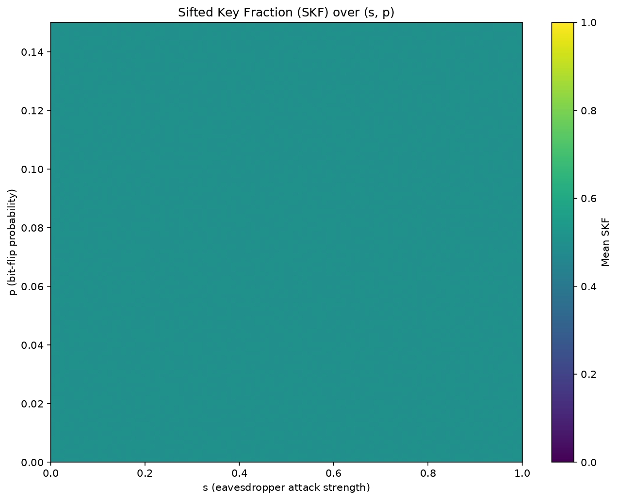
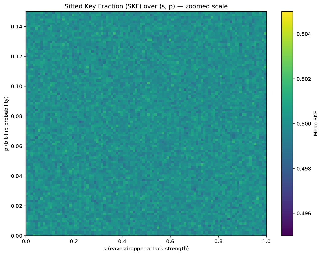
Figure 2 | SKF vs (s, p) averaged for each (s, p) pair

Across the 10 million trials, the minimum SKF was 0.413, and the maximum was 0.583. Averaging each (s,p) pair yields a minimum SKF of 0.49802 and a maximum of 0.50182. Across the 10 million trials, the standard deviation for SKF was 0.015810. The standard deviation for the averaged pairs, where each averaged pair was treated as a data point, was 0.000501. One-sample t-tests comparing the SKF to 0.5 were performed at each (s,p) pair with a significance level set at 5%. Out of 10,000 pairs, 518 rejected the null hypothesis, corresponding to a rejection rate of 5.18%. This rate of 5.18% closely matches the expected 5% false positive rate through chance from setting the significance level to 5%. The mean of the Cohen’s d value across the 10,000 pairs was 0.0253. The maximum Cohen’s d value for any pair was 0.1233. The benchmark for a small effect size using Cohen’s d is 0.20. Since both the mean and maximum values are well below this threshold, the difference between theory and simulation is negligible. Additionally, visually inspecting Figure 3 demonstrates a random scattering around the 0.500 average. This further supports that the SKF is independent of s and p.

QBER

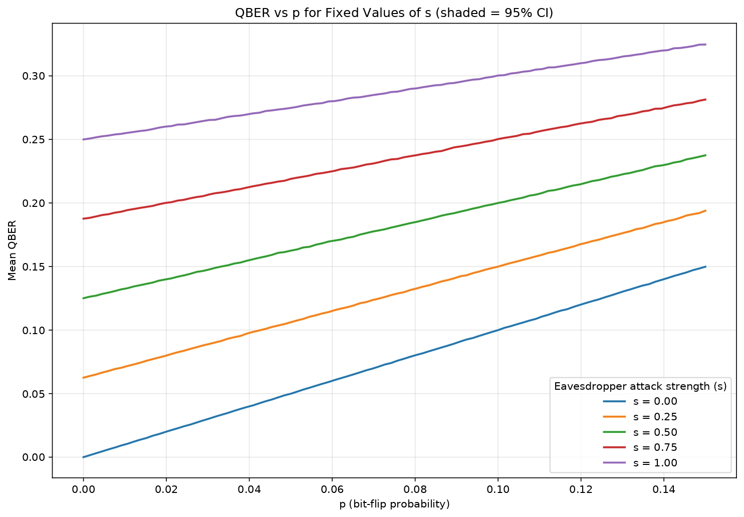
We now must look for a relationship between s, p, and QBER. First, s is held constant at 5 different values and the dependence of QBER on p is analyzed. For the five fixed values of s, we look at when s = 0, s = 0.25, s = 0.50, s = 0.75, and s = 1.

s Value	Fitted Slope + 95% CI	Theoretical Slope ( $1-\frac{s}{2}$ )	Fitted Intercept + 95% CI	Theoretical Intercept ( $\frac{s}{4}$ )	Slope % Difference	r²
0.00	1.0000, [0.9995, 1.0005]	1.0000	0.000, [-0.0000, 0.0001]	0.0000	0.0001%	0.999994
0.25	0.8747, [0.8740, 0.8754]	0.8750	0.0625, [0.0625, 0.0626]	0.0625	0.0327%	0.999985
0.50	0.7497, [0.7489, 0.7505]	0.7500	0.1250, [0.1249, 0.1251]	0.1250	0.0344%	0.999972
0.75	0.6251, [0.6242, 0.6260]	0.6250	0.1875 [0.1874, 0.1876]	0.1875	0.0102%	0.999949
1.00	0.5006, [0.4997, 0.5016]	0.5000	0.2500 [0.2499, 0.2501]	0.2500	0.1237%	0.999913

Table 1 | Fitted QBER vs Theoretical QBER.

The high r² values demonstrated by Table 1 indicate that all fitted lines are linear in p when s is constant. Additionally, the fitted slopes match closely to their predicted values, with the maximum discrepancy being only 0.1237%. Combining with the intercepts closely matching their theoretical predictions, this suggests that the model of QBER being linear in p when s is held constant has a high degree of accuracy. Additionally, it suggests that the equation for modeling QBER was accurate.

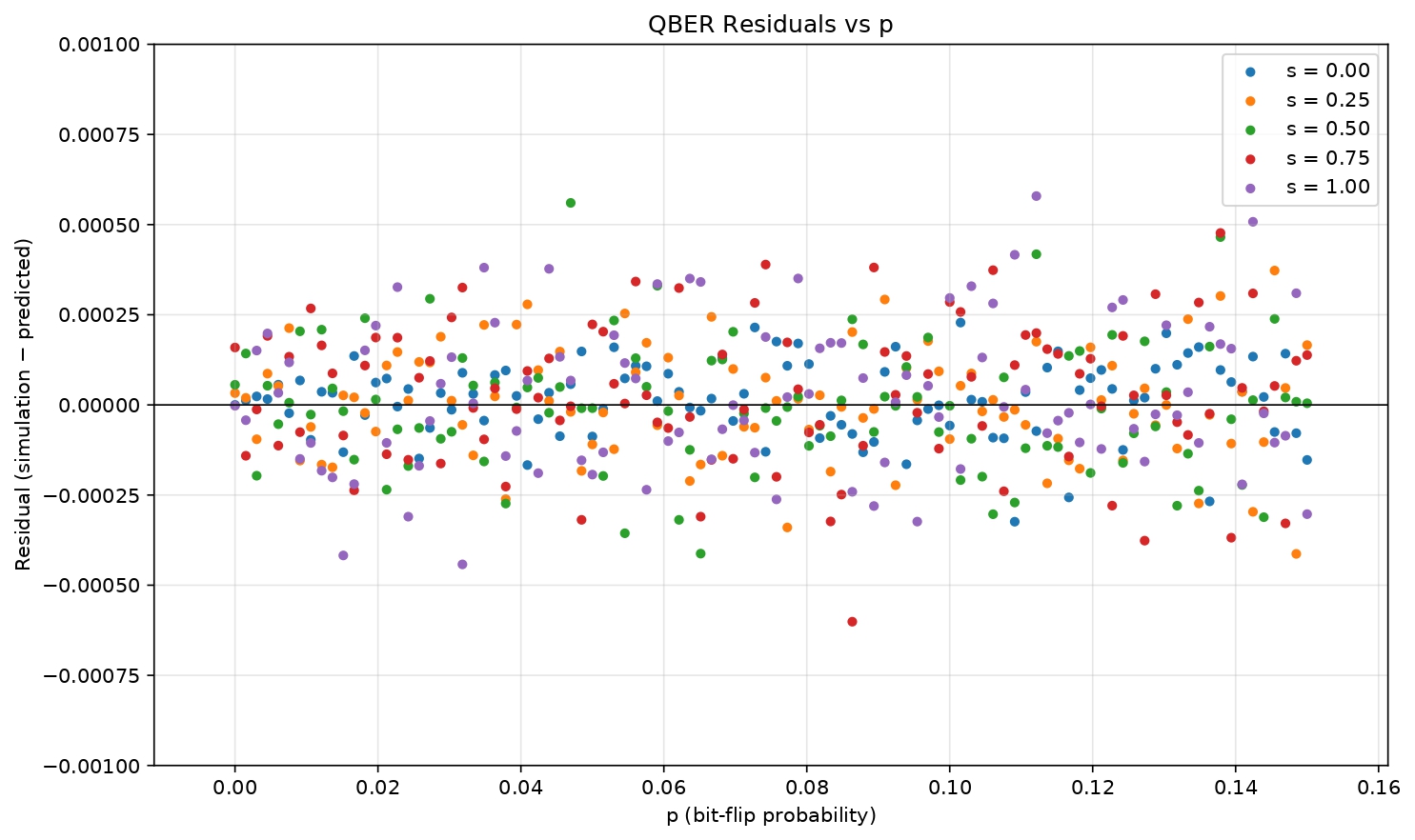
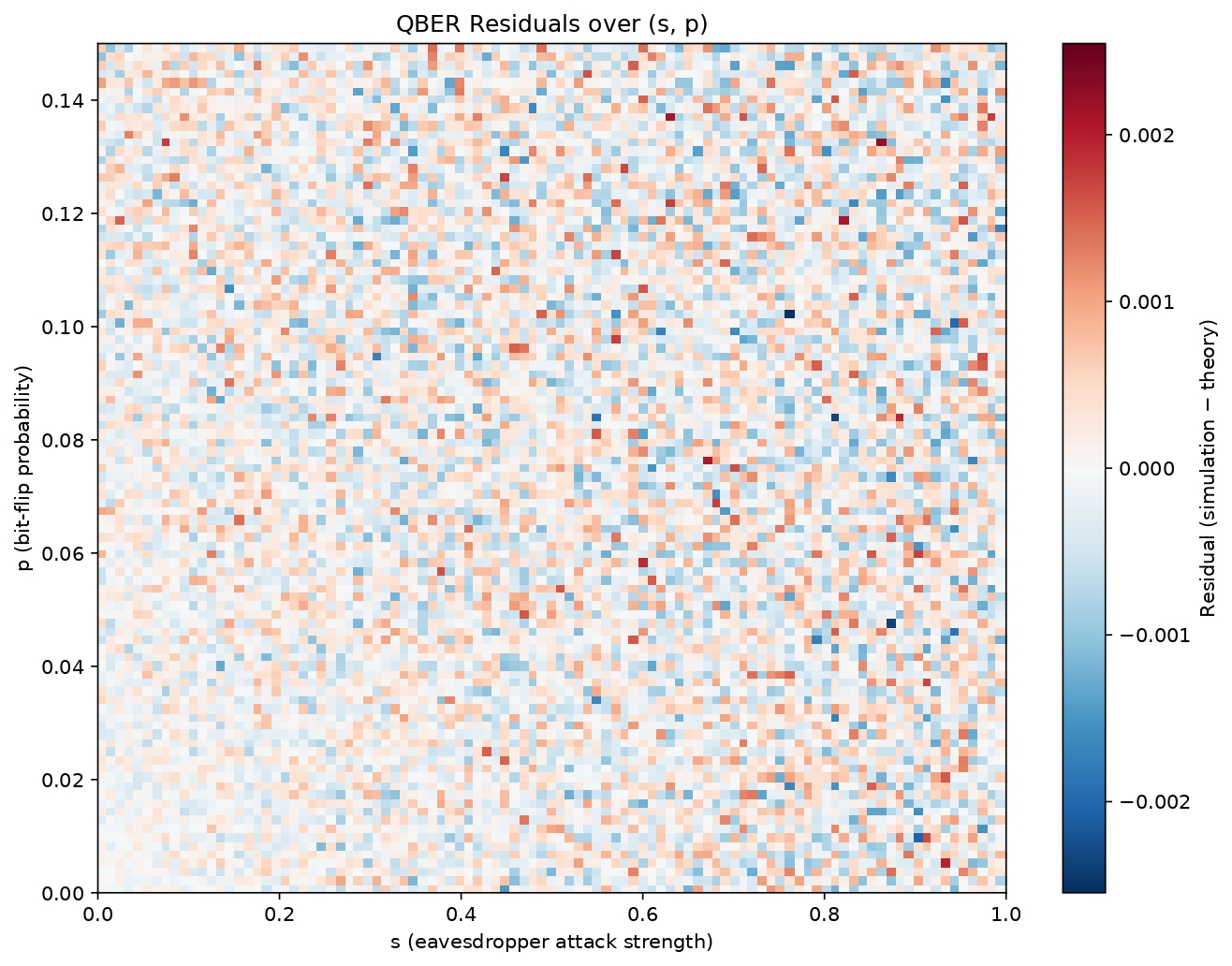
Figure 5 | QBER Residuals vs p for Fixed Values of s

The plot in Figure 5 of the residuals of the simulated results minus the predicted results showed a random scatter, with no visual curve or pattern. The mean residual was 0.000014, with a standard deviation of 0.000171. The random scattering indicates that the linear model accurately describes the QBER and is not overestimating or underestimating significantly. It supports that the small residuals result from finite noise rather than an incorrect model. However, there are also limits of having a finite number of bits.

s Value	1k Bit Slope	10k Bit Slope	Theoretical	1k Bit $r^2$	10k Bit r²
0.00	1.0000	1.0000	1.0000	0.999925	0.999994
0.25	0.8753	0.8747	0.8750	0.999866	0.999985
0.50	0.7509	0.7497	0.7500	0.999784	0.999972
0.75	0.6243	0.6251	0.6250	0.999523	0.999949
1.00	0.5003	0.5006	0.5000	0.999164	0.999913

Table 2 | 10,000 Bits vs 1,000 Bits QBER Simulation.

Through the general 10 million trial simulation, the difference between 1,000 bits and 10,000 bits can be compared. This will help demonstrate the finite-key effects in simulations. Among these values of s (except for s = 1.00), Table 2 demonstrates that cases with 10,000 bits are equal to or closer to the theoretical slope value and have a higher coefficient of determination than their 1,000 bits counterpart. This demonstrates the increasing linearity that comes with higher sample counts and higher key lengths, as well as the increasing accuracy of the model.

Next, we look to all combinations of (s,p) and how they impact the QBER.

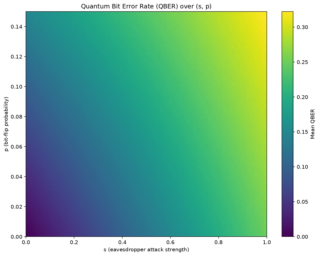
The heatmap of the QBER in Figure 6 demonstrates an increasing QBER as both error probabilities increase. The area of lowest QBER is near $(0, 0)$ , where both probabilities are lowest, and highest QBER near $(1, 0.15)$ , where both probabilities are near their maximum in the tested range. Running a residual test across all 10,000 points, the mean residual was 0.000001. The standard deviation was 0.000533, and the maximum absolute residual was 0.002546. The residuals are not significantly different from 0, as $t = 0.1763$ and $p = 0.860$ , indicating an unbiased model. Visually inspecting the residual heatmap for the QBER in Figure 7, the residuals appear randomly distributed. When the simulated QBER was fit to the predicted QBER, the $R^2$ value was 0.999943. When fit with least-squares regression to a bilinear model, the intercept was -0.000017, the $s$ coefficient was 0.2500, the $p$ coefficient was 1.0004, and the $sp$ coefficient was -0.5009. These closely match their predicted values of 0, 0.25, 1, and -0.5 respectively. This indicates that the predicted model is highly accurate and not overestimating or underestimating in particular areas. The matching of fitted coefficients also supports the accuracy of the predicted QBER.

SKR

Now that we have derived/validated QBER in terms of $s$ and $p$ and have confirmed the expected SKF value of 0.5, we can begin to analyze the SKR. We have the formula for SKR in terms of QBER, and now we can substitute QBER in terms of $s$ and $p$ .

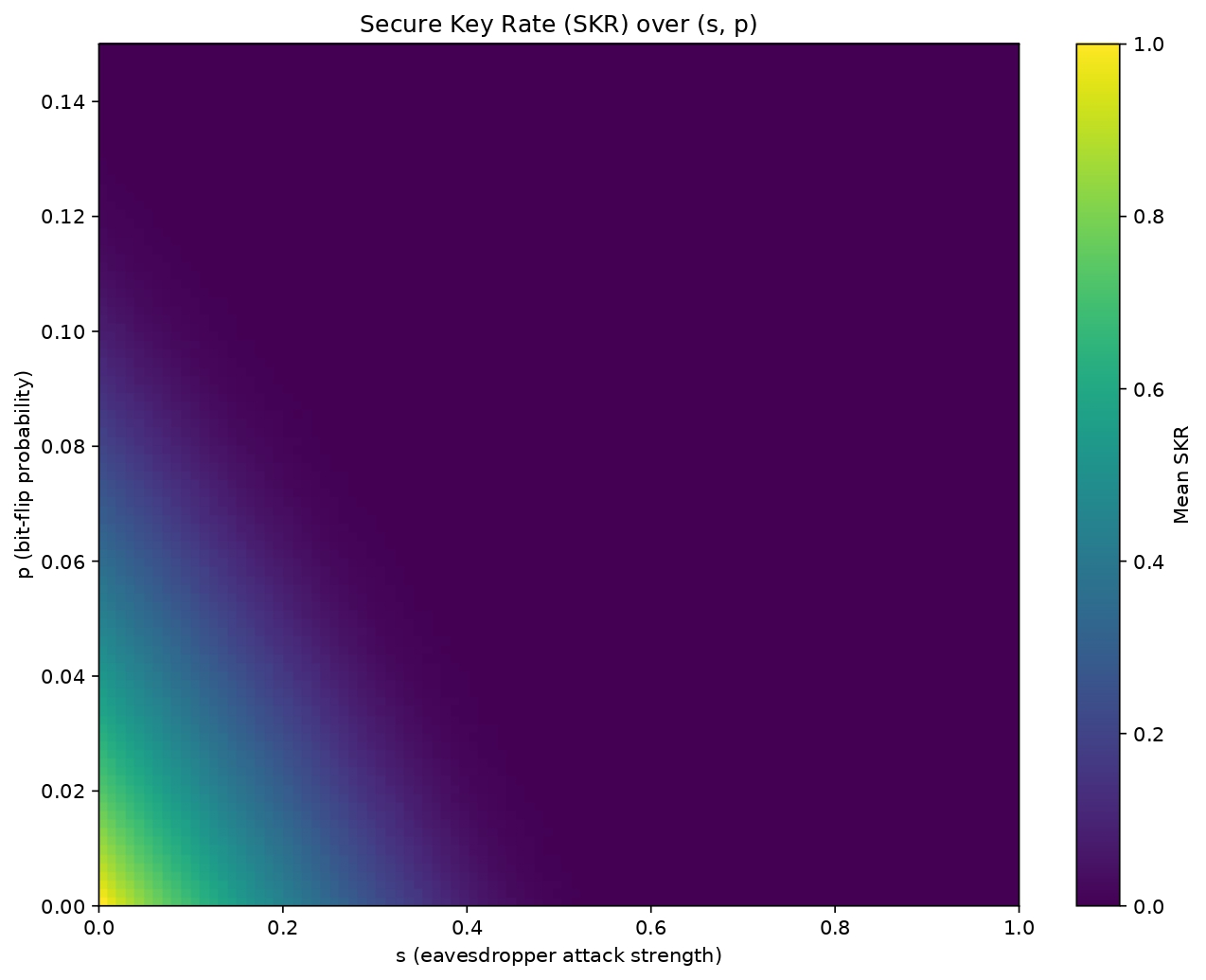
The SKR vs s and p in Figure 8 demonstrates a clear drop-off in value, being 0 for the majority of combinations of s and p. Ideally, there would be no error in communications. But if there were sufficient interference, it would cause an intolerable amount of error, ultimately causing the protocol to not yield a usable key. We want to determine the boundary for that cutoff. If the equation for SKR is set to 0, then we find 0=(1-(1+1)*H(QBER)). Solving for H(QBER) and subsequently finding the value of QBER that satisfies the equation yields QBER = 0.1100 or around 11%.

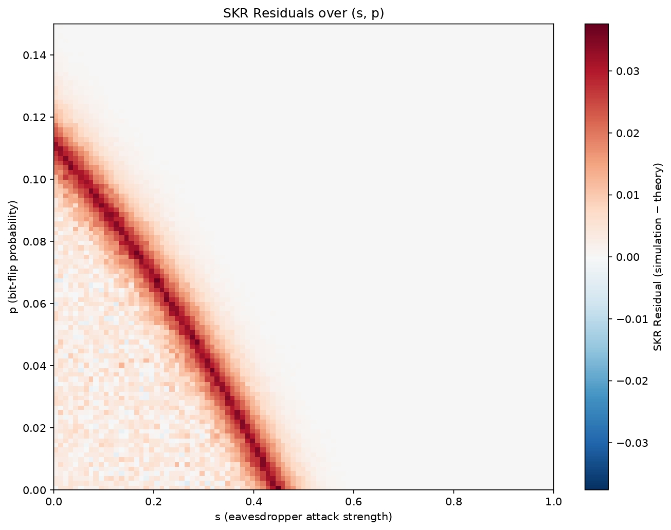
When analyzing the residuals, there are 137 negative residuals, 6118 residuals being exactly 0, and 3745 positive residuals. When plotted in Figure 9, a distinct red band can be identified on the boundary where the SKR becomes 0 and where QBER would be 11%. This is another example of the finite-key effects. Around the boundary, the simulation overestimates the SKR. At this point, rather than being averaged by negative and positive results, since the SKR function is strictly nonnegative, the trials below the QBER threshold yield a positive result, while the trials above yield 0 instead of a negative counterpart. This results in an overestimation. In an infinite key length limit, this effect would become negligible as the simulated results would approach the theoretical predictions. The negatives that occur here are valid. They occur from the finite number of trials and bits that may yield underestimated SKR values. But the frequency with which this happens is lower due to the minimum of a 0 value for SKR.

Sensitivity to f

This residual analysis was for f = 1. In implementations of BB84 and error correction algorithms, however, f is not equal to the ideal limit of 1. It can vary, and the effects of f will also be analyzed. When equating the maximum QBER with the derived formula for QBER, the boundary conditions can be found for which (s,p) exist on the maximal value of QBER.

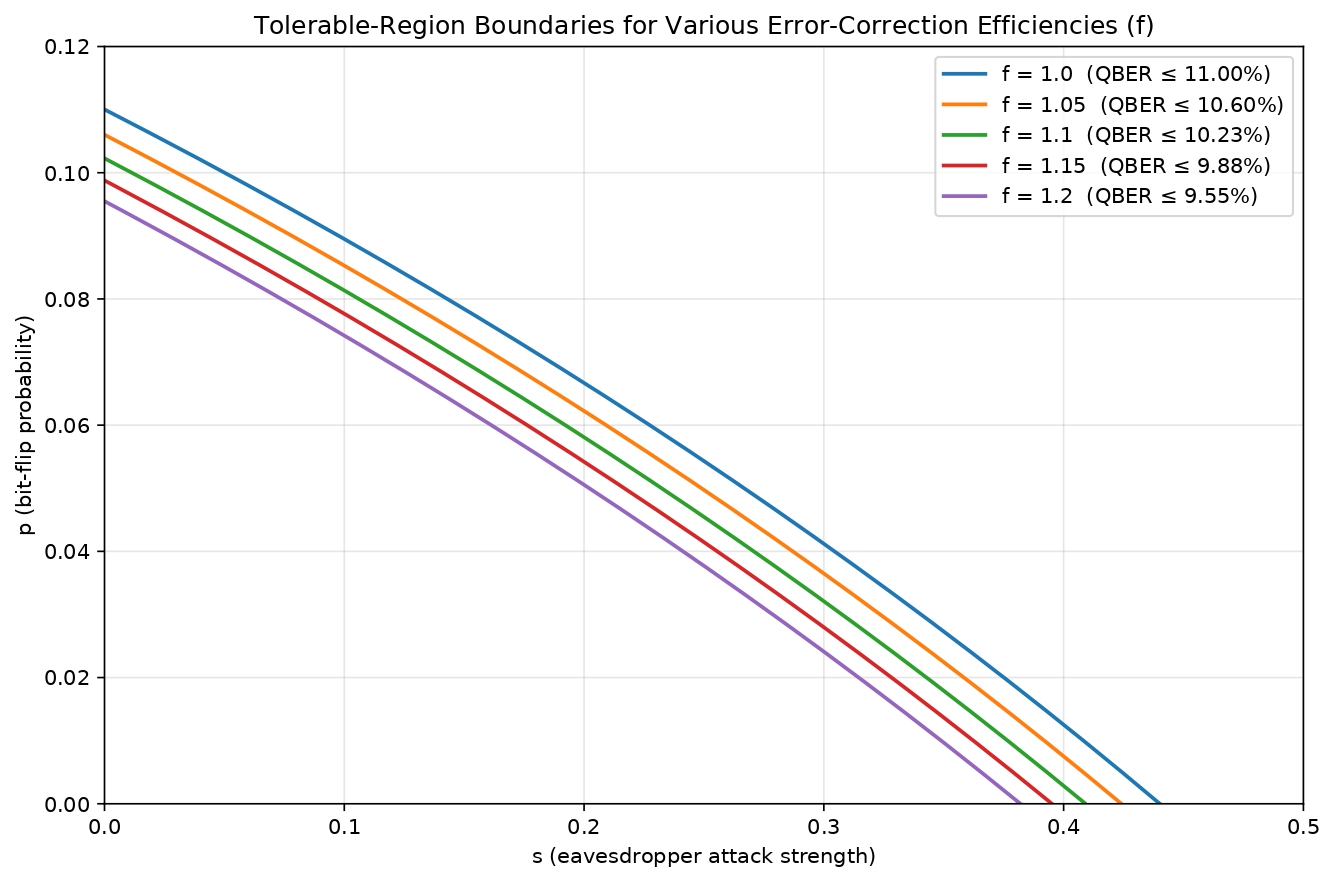
Figure 10 | Tolerable QBER Boundaries for Varying f

As $f$ increases, the maximum tolerable QBER continually decreases, representing a decreasing efficiency. Plotting the boundary conditions in Figure 10, they continually move inwards as $f$ increases, reflecting the decreasing maximum QBER. Thus, as the efficiency decreases, the maximum error from eavesdropping and natural noise that can be tolerated also decreases. This demonstrates the utility of error correction code that can efficiently run, as the higher efficiency can result in higher tolerances.

Discussion

Key Findings

As demonstrated by the simulations, the SKF does not significantly deviate from its theoretical value of 0.5. From analyzing the graph of QBER vs $p$ for select values of $s$ , the linearity of this relation was demonstrated. After comparing the theoretical slopes and intercepts to their simulated counterparts, the predicted model also shows high accuracy [Table 1]. The residuals demonstrated an unbiased model that randomly varied in terms of over or underestimating. When comparing how a different number of bits affects the data, the higher bit simulation tended to have a higher coefficient of determination and closer accuracy in terms of slope to the model. Looking across all 10,000 averaged data points, there is an increase in QBER as both $s$ and $p$ increase. There is an $R^2$ value of 0.999943 when fitting the simulated QBER to the theoretical model. Additionally, comparing the bilinear fitted coefficients and intercepts to the model’s prediction ( $QBER=(1-\frac{s}{2})p+\frac{s}{4}$ ) demonstrates extremely close alignment. Looking at the residuals, they are visually scattered and are statistically not significantly biased.

In the case of the SKR, the majority of points demonstrate a value of 0 and a decreasing SKR as both error sources increase. Analyzing the residuals of the SKR vs the predicted model, there are many more overestimations than underestimations, and a great number of perfect 0 residuals. A distinct red band appears where the QBER is 11%, demonstrating the effects of finite key length near the SKR cutoff.

When analyzing the boundary for multiple values of $f$ , the maximum QBER tolerable decreases while $f$ increases. As a result, the possible combinations of $s$ and $p$ also decrease, demonstrated by Figure 10.

The hypothesis of the linear relation between QBER and $p$ when $s$ is held constant was demonstrated, and the predicted bilinear model fit the simulation well. Additionally, the finite key effects upon simulation results were explored in the SKF and SKR, further demonstrating the limitations of simulation and finite bits.

Connections

This study analytically derives and empirically validates an explicit relation between eavesdropping, noise, and error rate in the form of $s$ , $p$ , and QBER. By establishing this relationship, the gap in simulation-based work of deriving a relation between error and performance can also be filled, using simulation to validate the analytically derived model. The simulations determined a QBER cutoff of around 11%, just as Shor and Preskill (2000) predicted, validating simulation against theory¹¹. In addition, the simulation validated the ability to predict the tolerable regions of $(s, p)$ for changing error correction efficiencies.

Regarding physical plausibility, real QKD implementations exhibit varying QBER values, but they are generally well below the range examined here. For instance, Guan et al. (2026) reported an average QBER of approximately 1.12% for a BB84 system deployed over a fiber network, well below both the 11% tolerable threshold and the maximum bit-flip probability of 0.15 examined in this simulation³³. Assuming no eavesdropper interference ( $s = 0$ ), where QBER equals $p$ , this 1.12% corresponds to a bit-flip probability of only $p = 0.012$ . Because this study focuses on mapping the full QBER relationship, the bit-flip probability was deliberately extended to 0.15, beyond the security-relevant threshold, even though lower values are typical of real-world systems. Simulating these higher values remains valuable for developing the complete relationship between QBER and the error parameters $s$ and $p$ .

Other QKD protocols such as E91 and SARG04 have different security mechanisms¹³. E91 uses violation of Bell’s inequality to ensure security, and SARG04 uses a different classical post-processing to protect against the photon-number-splitting attack. While BB84 has a maximum QBER of 11%¹¹, E91 actually compares the measured CHSH quantity $S$ against its ideal value of $-2\sqrt{2}$ rather than a QBER³⁴. Compared to the 11% of BB84, SARG04 has a one-way maximum bit error rate of 14.9%³⁵. All three protocols demonstrate different tolerances due to their differing assumptions and models.

This study also demonstrates a reproducible simulation methodology for further studying and analyzing QKD performance.

Looking at a simulation-based study done by Dhakal et al. (2025), similar key-length tradeoffs can be observed²⁵. Although other works have compared the effects of a finite number of bits within a single algorithm or across algorithms, there has been a lack of work testing first-principle models fit versus bit number. Su (2023) built a Monte-Carlo simulation procedure which estimated upper bounds on the secure key rates²⁴. In contrast, this study derived an explicit equation for the SKR in terms of the error inputs for the BB84 protocol, but also through a Monte-Carlo style simulation.

Limitations

Being simulation-based, there are assumptions in place that limit the scope of this study. First, the protocol implemented assumes an intercept-resend model of eavesdropping. There are other attack types and exploits that can be used by eavesdroppers, but this study focuses specifically on the intercept-resend attack. Additionally, equipment defects, transmission errors, and other forms of error are simplified under an umbrella term of natural error, specifically bit-flip probability. There are also a limited number of bits in this study, and this can result in finite-key effects like those observed in the SKR. Because the simulation uses a finite key length, the QBER is measured in the finite-key regime but substituted into the asymptotic (infinite-key) SKR formula. As shown by the SKR residuals near the boundary, this introduces a small overestimation of the secure key rate, an effect that would vanish in the true asymptotic limit.

Recommendations

Future simulation-based QKD studies could incorporate and model additional error types such as those discussed in the introduction to better approximate real-world conditions of BB84 as well as other QKD protocols like E91 or SARG04.

Closing Thoughts

As quantum computing continues to advance and place classical encryption protocols at risk, it is imperative to develop suitable replacements. As the realm of quantum cryptography continues to expand and find its way into communications, we must learn the best ways to use it and maintain its security.

References

A. M. Qadir, N. Varol. A review paper on cryptography. in 2019 7th International Symposium on Digital Forensics and Security (ISDFS) pg. 1–6, 2019, https://doi.org/10.1109/ISDFS.2019.8757514. [↩]
R. L. Rivest, A. Shamir, L. Adleman. A method for obtaining digital signatures and public-key cryptosystems. Communications of the ACM. Vol. 21, pg. 120–126, 1978, https://doi.org/10.1145/359340.359342. [↩]
G. Brassard. Brief history of quantum cryptography: a personal perspective. in IEEE Information Theory Workshop on Theory and Practice in Information-Theoretic Security, 2005. pg. 19–23, 2005, https://doi.org/10.1109/ITWTPI.2005.1543949. [↩]
D. Stucki, M. Legré, F. Buntschu, B. Clausen, N. Felber, N. Gisin, L. Henzen, P. Junod, G. Litzistorf, P. Monbaron, L. Monat, J.-B. Page, D. Perroud, G. Ribordy, A. Rochas, S. Robyr, J. Tavares, R. Thew, P. Trinkler, S. Ventura, R. Voirol, N. Walenta, H. Zbinden. Long-term performance of the swissquantum quantum key distribution network in a field environment. New Journal of Physics. Vol. 13, pg. 123001, 2011, https://doi.org/10.1088/1367-2630/13/12/123001. [↩]
T. Lugrin. One-time pad. in Trends in Data Protection and Encryption Technologies (eds V. Mulder, A. Mermoud, V. Lenders & B. Tellenbach) pg. 3–6, Springer Nature Switzerland, Cham, 2023, https://doi.org/10.1007/978-3-031-33386-6_1. [↩]
A. Carrasco-Casado, V. Fernández, N. Denisenko. Free-space quantum key distribution. in Optical Wireless Communications: An Emerging Technology (eds M. Uysal, C. Capsoni, Z. Ghassemlooy, A. Boucouvalas & E. Udvary) pg. 589–607, Springer International Publishing, Cham, 2016, https://doi.org/10.1007/978-3-319-30201-0_27. [↩]
C. H. Bennett, G. Brassard. Quantum cryptography: public key distribution and coin tossing. Theoretical Computer Science. Vol. 560, pg. 7–11, 2014, https://doi.org/10.1016/j.tcs.2014.05.025. [↩] [↩]
I. G. Koprinkov. Quantum superposition principle reformulation and collapse of wave function explanation. Romanian Journal of Physics. Vol. 70, pg. 104–104, 2025, https://doi.org/10.59277/RomJPhys.2025.70.104. [↩]
H.-K. Lo, H. F. Chau. Unconditional security of quantum key distribution over arbitrarily long distances. Science. Vol. 283, pg. 2050–2056, 1999, https://doi.org/10.1126/science.283.5410.2050. [↩]
D. Mayers. Unconditional security in quantum cryptography. Journal of the ACM (JACM). Vol. 48, pg. 351–406, 2001, https://doi.org/10.1145/382780.382781. [↩]
P. W. Shor, J. Preskill. Simple proof of security of the bb84 quantum key distribution protocol. Physical Review Letters. Vol. 85, pg. 441–444, 2000, https://doi.org/10.1103/PhysRevLett.85.441. [↩] [↩] [↩] [↩] [↩]
R. Renner, N. Gisin, B. Kraus. Information-theoretic security proof for quantum-key-distribution protocols. Physical Review A. Vol. 72, pg. 012332, 2005, https://doi.org/10.1103/PhysRevA.72.012332. [↩]
V. Scarani, H. Bechmann-Pasquinucci, N. J. Cerf, M. Dušek, N. Lütkenhaus, M. Peev. The security of practical quantum key distribution. Reviews of Modern Physics. Vol. 81, pg. 1301–1350, 2009, https://doi.org/10.1103/RevModPhys.81.1301. [↩] [↩] [↩]
M. Pereira, M. Curty, K. Tamaki. Quantum key distribution with flawed and leaky sources. Npj Quantum Information. Vol. 5, pg. 62, 2019, https://doi.org/10.1038/s41534-019-0180-9. [↩]
M. Dušek, M. Jahma, N. Lütkenhaus. Unambiguous state discrimination in quantum cryptography with weak coherent states. Physical Review A. Vol. 62, pg. 022306, 2000, https://doi.org/10.1103/PhysRevA.62.022306. [↩]
M. Curty, N. Lütkenhaus. Intercept-resend attacks in the bennett-brassard 1984 quantum-key-distribution protocol with weak coherent pulses. Physical Review A. Vol. 71, pg. 062301, 2005, https://doi.org/10.1103/PhysRevA.71.062301. [↩]
S. Weigert. No-cloning theorem. in Compendium of Quantum Physics (eds D. Greenberger, K. Hentschel & F. Weinert) pg. 404–405, Springer, Berlin, Heidelberg, 2009, https://doi.org/10.1007/978-3-540-70626-7_124. [↩]
F. Xu, X. Ma, Q. Zhang, H.-K. Lo, J.-W. Pan. Secure quantum key distribution with realistic devices. Reviews of Modern Physics. Vol. 92, pg. 025002, 2020, https://doi.org/10.1103/RevModPhys.92.025002. [↩]
Á. Schranz, E. Udvary. Quantum bit error rate analysis of the polarization based bb84 protocol in the presence of channel errors: in Proceedings of the 7th International Conference on Photonics, Optics and Laser Technology pg. 181–189, SCITEPRESS – Science and Technology Publications, Prague, Czech Republic, 2019, https://doi.org/10.5220/0007384101810189. [↩]
R. Fang, V. V. Nikulin. Causes of bit error and error correction for quantum key distribution protocols. in Quantum Nanophotonic Materials, Devices, and Systems 2019 Vol. 11091 pg. 79, SPIE, 2019, https://doi.org/10.1117/12.2527763. [↩]
N. Gisin, G. Ribordy, W. Tittel, H. Zbinden. Quantum cryptography. Reviews of Modern Physics. Vol. 74, pg. 145–195, 2002, https://doi.org/10.1103/RevModPhys.74.145. [↩]
M. Tomamichel, C. C. W. Lim, N. Gisin, R. Renner. Tight finite-key analysis for quantum cryptography. Nature Communications. Vol. 3, pg. 634, 2012, https://doi.org/10.1038/ncomms1631. [↩]
M. Pereira, G. Currás-Lorenzo, Á. Navarrete, A. Mizutani, G. Kato, M. Curty, K. Tamaki. Modified bb84 quantum key distribution protocol robust to source imperfections. Physical Review Research. Vol. 5, pg. 023065, 2023, https://doi.org/10.1103/PhysRevResearch.5.023065. [↩]
H.-Y. Su. Monte carlo approach to the evaluation of the security of device-independent quantum key distribution. New Journal of Physics. Vol. 25, pg. 123036, 2023, https://doi.org/10.1088/1367-2630/ad141a. [↩] [↩]
P. Dhakal, B. R. Dawadi, N. B. Adhikari. Performance analysis of different quantum key distribution protocols for optimised security and efficiency. IET Quantum Communication. Vol. 6, pg. e70015, 2025, https://doi.org/10.1049/qtc2.70015. [↩] [↩]
D. Bunandar, L. C. G. Govia, H. Krovi, D. Englund. Numerical finite-key analysis of quantum key distribution. Npj Quantum Information. Vol. 6, pg. 104, 2020, https://doi.org/10.1038/s41534-020-00322-w. [↩]
K. Gkouliaras, V. Theos, P. G. Evans, S. Chatzidakis. NuQKD: a modular quantum key distribution simulation framework for engineering applications. Advanced Physics Research. Vol. 3, pg. 2400016, 2024, https://doi.org/10.1002/apxr.202400016. [↩]
M. H. Saeed, H. Sattar, M. H. Durad, Z. Haider. Implementation of qkd bb84 protocol in qiskit. in 2022 19th International Bhurban Conference on Applied Sciences and Technology (IBCAST) pg. 689–695, 2022, https://doi.org/10.1109/IBCAST54850.2022.9990073. [↩]
A. Adu-Kyere, E. Nigussie, J. Isoaho. Quantum key distribution: modeling and simulation through bb84 protocol using python3. Sensors. Vol. 22, pg. 6284, 2022, https://doi.org/10.3390/s22166284. [↩]
G. Bebrov. On the (relation between) efficiency and secret key rate of qkd. Scientific Reports. Vol. 14, pg. 3638, 2024, https://doi.org/10.1038/s41598-024-54246-y. [↩] [↩]
C. E. Shannon. A mathematical theory of communication. The Bell System Technical Journal. Vol. 27, pg. 379–423, 1948, https://doi.org/10.1002/j.1538-7305.1948.tb01338.x. [↩]
D. Tupkary, N. Lütkenhaus. Using cascade in quantum key distribution. Physical Review Applied. Vol. 20, pg. 064040, 2023, https://doi.org/10.1103/PhysRevApplied.20.064040. [↩]
R. Guan, J. Yu, Z. Li, H. Xie, Y. Wei, S. Li, J. Wen, X. Liang, Y. Li, K. Wei. Field-trial quantum key distribution with qubit-based frame synchronization. Optics Express. Vol. 34, pg. 16677–16686, 2026, https://doi.org/10.1364/OE.593410. [↩]
A. K. Ekert. Quantum cryptography based on bell’s theorem. Physical Review Letters. Vol. 67, pg. 661–663, 1991, https://doi.org/10.1103/PhysRevLett.67.661. [↩]
C.-H. F. Fung, K. Tamaki, H.-K. Lo. Performance of two quantum-key-distribution protocols. Physical Review A. Vol. 73, pg. 012337, 2006, https://doi.org/10.1103/PhysRevA.73.012337. [↩]