
Abstract
This study conducted a statistical analysis of CMOS sensor noise and investigated its impact on the navigational accuracy and stabilityof a mobile robot under varying illuminance. While passive optical sensors are the primary drivers of autonomous navigation, their data fidelity and performance are impacted by stochastic noise mechanisms. Using a customized robotic platform equipped with an OV2640 sensor, this research quantified performance across four illuminance tiers, ranging from 0 to 533.33 lux. The investigation utilized Root Mean Square Error (RMSE) to measure absolute accuracy and Standard Deviation (SD) to isolate stability (temporal “navigation jitter”). The results identified a non-linear error curve, showing that peak performance (RMSE = 2.44 cm; SD = 0.15 cm) was restricted to a controlled 53.33-lux environment. At the 0-lux floor, Read Noise entirely consumed the signal, leading to a total loss of spatial coordinate precision (p<0.001). At the 533.33-lux ceiling, Full Well Capacity saturation and pixel blooming caused a statistically significant degradation in both accuracy and stability (p=0.001). The integration of Independent Samples t-tests confirmed the repeatability of these findings, proving that deviations were deterministic outcomes of CMOS noise mechanisms rather than random mechanical error. The study concluded that robotic navigational precision was a non-linear function of ambient illuminance, dictated by the sensor’s ability to maintain data fidelity within an optimal photometric window.
Keywords: Illuminance, CMOS Sensor Noise, Root Mean Square Error, Photometric Window, Stochasticity, Blooming, Inferential Statistics.
Introduction
Last decade has witnessed increasing usage of Complementary Metal-Oxide-Semiconductor (CMOS) sensor technology in mobile and smart phones1. Further, the rapid advancement in autonomous mobile robotics has necessitated efforts to enhance sophistication of vision-based navigation systems, wherein the CMOS sensor serves as the primary source of vision, translating environmental light into digital data for real-time decision-making2,3.
As CMOS technology has become the industry standard for optical sensors, such as the OV2640, due to its low power consumption, high resolution, and ability to provide stable pixel data through efficient transistor logic, this study tried to investigate the impact of varying illuminance on CMOS sensor based mobile robots4,5.
The complementary nature of CMOS refers to its use of paired NMOS (Negative-channel) and PMOS (Positive-channel) transistors. These transistors react in opposite ways to a voltage signal: when an NMOS transistor turns ON to conduct at a High voltage (Logic 1), the PMOS stays OFF, and vice versa. This configuration ensures that the sensor’s output is always hard connected to either Power or Ground, which prevents minor electronic fluctuations from distorting the “Highs” and “Lows” of the pixel data ensuring signal stability required for consistent digital interpretation in variable environments.
Although the architectural design of CMOS inherently attempts to provide a stable digital foundation, yet as these sensors function by converting incoming photons into an electrical charge, their ultimate performance is heavily dictated by the Signal-to-Noise Ratio (SNR). SNR measures the ratio of signal strength (illuminance) to the background noise level6,7,8.
Each lighting environment triggers specific noise mechanisms that can override the sensor’s hard-connected stability. The study identified and analyzed various possible sources of SNR that impacted path precision of a CMOS sensor-mounted-moving-vehicle. The research aimed to transition from optical physics to autonomous navigation by discussing the digital noise in mobile robotics and exploring the relationship between optical data fidelity and mechanical performance. Within the context of this study, data fidelity is defined as the degree of correlation between the physical coordinates of the navigation track and the digitized coordinates generated by the CMOS sensor. High data fidelity implies an image where the Signal-to-Noise Ratio (SNR) is high enough to prevent stochastic pixel fluctuations from shifting the calculated centroid of the track.
The primary objective of this study was to conduct a statistical analysis of CMOS sensor noise and RMSE path deviation in a mobile robot under diverse illuminance levels. To achieve this, the research specifically aimed to quantify the Root Mean Square Error (RMSE) of a mobile robot’s path deviation across four distinct levels of ambient illuminance and calculated the Standard Deviation (SD) of the robot’s lateral position to isolate the impact of temporal noise. This metric serves to quantify navigational jitter, defined as the high-frequency steering oscillations that degrade mechanical precision. The study analyzed the results by evaluating how various noise mechanisms, both spatial and temporal, specifically Read Noise, Photon Shot Noise, and Photo Response Non-Uniformity (PRNU), impacted the sensor’s ability to maintain a stable trajectory. Finally, t-tests were conducted to determine the statistical significance of illuminance-induced errors on mechanical precision, assessing both the absolute accuracy of the robot and its navigational stability under varying photometric constraints.
In analyzing these effects, CMOS sensor noise was categorized into two primary domains: Temporal Noise, which fluctuates over time and is often signal-dependent, and Spatial Noise, which remains constant across the sensor array (signal-independent). The functional range of the CMOS sensor is bounded by the two domains: the “illuminance ceiling” as determined by the Full Well Capacity (FWC), and the “noise floor” as dictated by Read Noise.
The Noise Ceiling: Full Well Capacity leading to saturation and blooming
FWC represents the maximum amount of charge (number of electrons) a single pixel can hold before it reaches saturation and blooming, thereby disrupting data fidelity of the sensor. While it is not a noise in theoretical sense, it does impact the function of CMOS sensors at higher illuminance. When a photon hits the silicon of a pixel, it generates an electron through the photoelectric effect. These electrons are stored in a potential well (a “storage area”) within the pixel. The physical size and voltage of the pixel determine its depth. Once saturated, it cannot accurately count any more incoming light. Each sensor device has a specific Full Well Capacity depending on the pixel size (e.g., 2.2µm for this study) that impacts signal to noise ratio and the data fidelity. As the maximum signal S is capped by the FWC, the maximum achievable SNR is also capped. When a pixel exceeds its FWC, the excess electrons often leak into neighboring pixels. This is called Blooming that causes the edges of an object to “bleed” or blur into adjacent pixels, giving an inaccurate spatial reading, resulting in inaccurate spatial readings and increased RMSE.
The Noise Floor: Read Noise and the Readout Phase
Conversely, Read Noise defines the sensor’s “noise floor,” establishing the minimum detectable signal required to maintain data fidelity. Read noise is a temporal phenomenon occurring during the readout phase, where accumulated electrons are transferred from the pixel to the Analog-to-Digital Converter (ADC). The sensor must turn a physical voltage (analog) into a number (digital). Read noise is essentially the “measurement error” that happens during that translation. If the light signal is lower than the read noise, the visual data is obscured by electronic “fuzz.” In this study, read noise is attributed to three primary stochastic behaviors9.
1. Thermal Agitation (Johnson-Nyquist Noise): Caused by the random heat-induced movement of electrons within the amplifiers and resistors of the OV2640 sensor, creating fluctuating voltages.
2. Flicker Noise (1/f Noise): Originating from impurities in the CMOS transistors’ conductive channels, where electrons are randomly trapped and released.
3. Quantization Error: A digital rounding discrepancy occurring when the ADC converts continuous analog voltage into discrete digital integers (binary 0s and 1s). This rounding creates a tiny, random error in every measurement, manifesting as jitter in the robot’s perception.
The Intermediate Range
Between the extremes set by FWC and Read Noise, lies Photon Shot Noise and Photo Response Non-Uniformity (PRNU), which fluctuate with light levels and introduce spatial inaccuracies.
Photon Shot Noise (The Dominant Signal-Dependent or Temporal Noise)
Shot noise is a type of random noise that is a fundamental property of light itself, not the sensor hardware. It is the outcome of photon fluctuation and can result in less accurate and less reliable data. As the light arrives as a stream of discrete photons, it follows a Poisson distribution.
(1) 
Where N is the noise and S is the signal or number of collected photons
As illuminance or signal increases, the absolute amount of noise increases (more photons = more random fluctuation), but the Signal-to-Noise Ratio (SNR) improves because the signal grows linearly while the noise only grows by the square root. However, after the sensor reaches its saturation under high illuminance, shot noise limits data fidelity, overriding electronic read noise.
Photo Response Non-Uniformity (PRNU) (Spatial/Fixed-Pattern)
PRNU is a form of Fixed Pattern Noise (FPN) that occurs because every pixel has a slightly different sensitivity to light10,11.
It is a spatial phenomenon caused by microscopic variations in the sensitivity of individual pixels. While PRNU is signal-dependent, meaning it is non-existent in total darkness, it is not temporal; the pattern remains constant across every frame.
As the ambient illuminance is increased, the spatial “fixed” variations between pixels become more pronounced, decreasing spatial precision. This is because the sensor perceives “textures” or patterns in the illuminance that don’t exist in the environment.
Since the study analyzed a path-following task of CMOS rather than just taking photos, it was critical to understand how optical noise became sources of steering fluctuations.
To analyze the data collected from the mobile robot, three primary statistical lenses were employed to distinguish between constant error and unpredictable instability.
Root Mean Square Error (RMSE): The Metric for Path Accuracy or deviation from the Path
RMSE served as the primary metric for overall accuracy12.By squaring the deviations before averaging, RMSE noted where the robot significantly deviated from the prescribed path. It represents the combined effect of both the sensor’s accuracy and the robot’s mechanical response.
(2) 
where:  is the total number of data points (measurements) collected during the trial;
  is the deviation or difference between actual measured value,
  and the predicted value
  (center of the prescribed 4.5cm black tape);
  is the sum of the squared deviations.
Standard Deviation (SD): The Metric for Navigational Jitter or Instability
While RMSE showed how far the robot was from the center, the Standard Deviation specifically measured the consistency of that error. A high SDwas a direct mechanical manifestation of Temporal Read Noise, while a low SD indicated a stable movement.
(3) 
where: is the total number of data points (measurements) collected during the trial;  is the RMSE at each specific trial and
  is the mean of RMSE across 10 trials for each of the 4-illuminance level.
As the study sought to understand to what extent does varying ambient illuminance affect the navigational precision (measured via RMSE and Standard Deviation) of a CMOS-based mobile robot, it was hypothesized that the robot’s path-following accuracy would follow a non-linear correlation with illuminance levels. Under low illuminance, RMSE and Standard Deviation would increase significantly as the signal dropped toward the Read Noise Floor, causing temporal jitter whereas in high illuminance the accuracy would again degrade as pixels reached FWC, leading to blooming and loss of edge definition. There would be an optimal medium illuminance level where the SNR would bemaximized, resulting in the lowest RMSE and SD.
T-test: The Metric for Statistical Significance or Repeatability
While Descriptive Statistics (RMSE and SD) summarized what happened during the trials, the Independent Samples t-test was employed to determine statistical significance. Its primary role was to evaluate the Null Hypothesis (H0), which assumed that varying illuminance levels would have no measurable impact on the robot’s mechanical precision and Alternative Hypothesis (Ha), which assumed that changes in ambient illuminance would have a statistically significant impact on the robot’s RMSE and SD. By comparing the means of two independent groups (e.g., Control vs. Highest Illuminance), the t-test calculated the probability (p-value) that the observed increase in RMSE and navigation jitter was caused by the manipulated noise variables (Photon Shot Noise and Blooming) rather than stochastic motor fluctuations.
The scope of this study was focused on the interaction between ambient illuminance and the OV2640 CMOS sensor (2.2µm pixel size) within the context of a dynamic path-following task. The experimental environment was limited to a wooden cardboard substrate and a 295.12 cm black tape path. However, the study was subject to limitations imposed by mechanical variables, surface texture and resource constraints. Factors such as, motor torque, and wheel friction were assumed to be constant throughout the 10 trials. The natural grain of the wooden cardboard might have introduced minor spatial noise that could impact RMSE at extreme light levels. The research evaluated a specific sensor model and might not fully represent the behavior of sensors with different Full Well Capacities or pixel architectures. The study was conducted in an indoor environment, and the findings are not indicative of sensor performance in an outside environment, under natural light.
Methodology
Set-Up
The experiment utilized a customized autonomous platform where high-level computation and motor coordination were managed by a Raspberry Pi 5 (8GB RAM)13,14,15. This unit interfaced with an Arduino Uno via serial communication to drive four DC geared motors through an L298N dual H-bridge motor driver. Environmental perception was provided by an ESP32-CAM module equipped with an OV2640 CMOS image sensor, mounted at a fixed forward-facing angle to maintain a constant field of view. To ensure spectral consistency, a 5600K (Daylight Balanced) LED array served as the light source. The vehicle was deployed from a standardized starting position for each trial, with navigational data processed in real-time to determine the path deviation metrics.
Experimental Design and Variables
A single-variable experimental design was employed, with ambient illuminance (lux) serving as the primary independent variable. Testing was conducted across four discrete photometric tiers—0, 53.33, 213.33, and 533.33 lux—with ten full-circuit trials per condition (n=40 total trials). The Root Mean Square Error (RMSE) of the vehicle’s lateral path deviation served as the dependent variable, quantifying navigational precision. To isolate the effects of light intensity, several parameters were strictly controlled: motor voltage (and thus velocity) was kept constant, and all Image Signal Processor (ISP) features on the sensor, including Autoexposure (AEC) and Auto-Gain (AGC), were locked to prevent algorithmic compensation for lighting changes.
Environmental Controls and Photometric Calibration
The experiment was conducted in a light-controlled indoor environment to eliminate external variables such as infrared interference from sunlight16. Four controlled photometric tiers were established to represent the spectrum of the optical photometry window. These levels were derived by distributing the luminous flux (0, 120, 480, and 1200 lumens) over a standardized testing area, resulting in four specific illuminance levels: 0 lux, 53.33 lux, 213.33 lux, and 533.33 lux. The 53.33-lux environment was designated as the experimental control to represent the sensor’s optimal dynamic range. The control condition of 53.33 lux was selected based on the OV2640 manufacturer specifications, which define a 2.2µm pixel architecture and a maximum SNR of 40 dB. This illuminance level ensures the sensor operates within its Linear Dynamic Range, providing a sufficient photon count to exceed the Read Noise floor without inducing the Full Well Capacity saturation and Blooming typically observed at higher intensities (e.g., 533.33 lux). Consequently, 53.33 lux served as a baseline for high data fidelity before the introduction of signal-dependent artifacts.
Algorithmic Consistency and Perception Framework
Hue, Saturation, Value (HSV) thresholds were determined empirically under the control condition (53.33 lux) to define the ‘Optimal Detection Window’17. Crucially, the HSV threshold values were kept constant across all experimental tiers. The algorithm was not optimized for each lighting condition; this was a deliberate design choice to ensure that any navigational error observed at 0 lux or 533 lux was a result of sensor data degradation rather than variations in algorithmic sensitivity.
Control Logic and Kinematic Standardization
The robot’s steering was governed by the same motor calibration across trials ensuring that any increase in Standard Deviation or RMSE was caused by optical noise, such as Read Noise or Pixel Blooming, rather than fluctuations in the steering algorithm. The algorithm calculated the horizontal offset (e) of the track’s center of mass relative to the camera’s optical axis. This offset is then processed by a Proportional-Integral-Derivative (PID) controller to determine steering adjustments14.
This controlled kinematic approach was essential to ensure that any observed fluctuations in spatial coordinate precision, specifically RMSE and Standard Deviation, were the result of photometric variables rather than mechanical acceleration or deceleration. To validate this, an Independent Samples t-test was integrated into the analytical framework; this allowed for a formal comparison between the control and experimental groups, mathematically determining if the changes in mechanical precision were statistically significant consequences of CMOS sensor noise rather than stochastic operational errors.
Statistical Analysis Framework
The study defined navigational precision, as navigational accuracy defined by the extent to which the robot adhered to the prescribed path in each trial; dynamic stability, that is the robot’s ability to avoid jitters and stay on course, navigational repeatability, that is how often the robot adhered to the prescribed path across trials at each illuminance level, as indicated in Table 1.
| Concepts | Alternative Term | Statistical Link |
| Accuracy | Deviation from Path | RMSE |
| Stability | Navigational Jitter | Standard Deviation |
| Repeatability | Path Fidelity | Comparative t-test |
Navigation path
The testing environment consisted of a 300×300 cm sanded and unpainted light cream plywood surface, chosen for its consistent texture and neutral reflectance. The navigation path was constructed using 4.5 cm wide black tape as indicated in Figure 1. The path and the substrate remained unchanged across trials to ensure that the hue, saturation and view (HSV) thresholding parameters remained constant across all four illuminance tiers to eliminate software-induced bias. This approach followed the standard “benchtop test” protocol for evaluating hardware reliability, as it forced the system to rely entirely on the sensor’s raw photometric output.
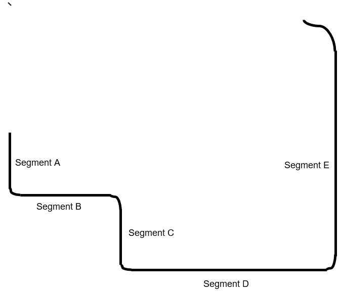
The path began at a designated ‘Origin Point’ and followed a sequence designed to test both linear stability and centripetal edge-tracking.
Total Length Calculation
- Total Linear Distance: 29+29+39+44+85=226 cm
- Total Curved Distance: 12.57+12.57+43.98=69.12 cm
Total Path Length: 226+69.12=295.12 cm (or approximately 2.95 meters).
Path Sequence Breakdown:
- Segment A: A 29 cm straight line. This served to stabilize the robot’s velocity before the first turn.
- Turn 1 (Tight Cornering): A quarter-circle curve with an 8 cm radius. This tested the sensor’s ability to handle rapid pixel state changes.
- Segment B (Intermediate Straight): A 29 cm straight line to allow the PID controller to re-center.
- Turn 2 (Reverse Cornering): A second quarter-circle curve with an 8 cm radius, oriented to test steering symmetry.
- Segment C (Approach): A 39 cm straight line leading into the complex steering section with a soft turn leading to Segment D.
- Segment D (Soft Maneuver): A 44 cm segment with a soft turn to Segment E. These helped Standard Deviation analysis, as low-intensity jitter was most visible during these subtle corrections.
- Segment E (High-Speed Straight): An 85 cm long straightaway. This allowed the robot to reach its maximum consistent velocity, testing the Signal-to-Noise Ratio (SNR) under high-frequency vibration.
- Final Turn (The “Omega” Curve): A semi-circular path with a 14 cm radius. This sustained turn was the primary site for observing Blooming and PRNU (Photo Response Non-Uniformity), as the sensor needed to process and correctly follow a constantly shifting field of view.
Error Metrics and Inferential Analysis
As the study aimed to identify the specific breakdown points of the CMOS sensor (the Read Noise floor and the Full Well Capacity ceiling), an Independent Samples t-test: was selected as the primary inferential tool. This allowed for a direct comparison between the Ideal lighting control and the experimental extremes.
The dependent variables were operationalized as follows:
Root Mean Square Error (RMSE): Used as the primary metric for navigational accuracy. It was calculated by comparing the robot’s actual spatial coordinates against the idealized center of the 4.5 cm tape path. By squaring the deviations, RMSE disproportionately weights larger “veering” events, representing the total magnitude of path error.
Standard Deviation (SD): Used to quantify navigational stability and “navigation jitter.” This metric measures the consistency of the robot’s lateral position relative to its own mean trajectory. A high SD indicates steering fluctuations induced by temporal sensor noise, such as Photon Shot Noise, which causes the robot to oscillate around the path.
Independent Samples t-test: This was used as the primary tool for inferential statistics to determine if the differences in RMSE and SD across lighting conditions were statistically significant. By comparing the means of the experimental trials against the control (53.33 lux), the t-test calculated a p-value to establish whether the observed mechanical degradation was a direct result of CMOS noise (such as FWC saturation) or merely the product of stochastic, random variation.
Degrees of Freedom (df): Since there were 10 trials per group, the degree of freedom (df) was (n1+n2−2) was 18.
By calculating a p-value, the t-test exceeded the 95% confidence interval allowing the study to distinguish between random mechanical fluctuations and errors directly induced by CMOS sensor noise (such as Photon Shot Noise and Blooming). This ensured that the identified ‘Optimal Photometric Window’ was a mathematically valid boundary rather than a result of stochastic outliers.
Results
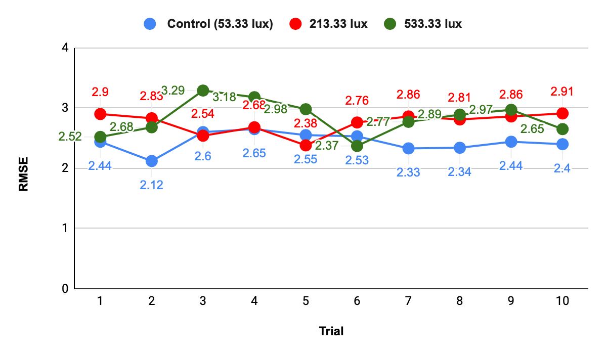
The robotic set up completed 10 trials at each illuminance levels resulting in a total of 40 trials, with each trial starting at the same specific coordinate on the path. The data revealed a system failure at the lowest illuminance of 0 lux or complete darkness, resulting in statistical measure of RMSE possible for the remaining 30 trials across three illuminance levels of 53.33 lux, 213.33 lux and 533.33 lux, as indicated in Figure 2.
The Minimum Illuminance Condition (0 Lux) At the absolute minimum of the experimental range (0 lux), the robotic platform experienced immediate and total system failure. In this state, the absence of incident photons meant that the OV2640 sensor was operating entirely beneath its 1.69-lux noise floor, where stochastic Read Noise completely overwhelmed any potential signal. Consequently, the edge-detection algorithm was unable to resolve the spatial coordinates of the path. As no successful trials could be completed at this level, 0 lux represented the physical boundary of navigational possibility for this sensor architecture. This categorical failure was found to be statistically significant (p<0.001) compared to the control, confirming that a minimum threshold of light is required to generate sufficient signal to transcend the baseline electronic noise of the OV2640 sensor.
The Optimal Control Condition (53.33 Lux) The 53.33-lux environment provided the optimal photometric window. At this level, the photon flux was sufficient to overcome Read Noise, while the impacts of Photo Response Non-Uniformity (PRNU) remained negligible. The robot achieved its peak stability with an average RMSE of 2.44 cm and a Standard Deviation of 0.15 cm. During the 8 cm radius curves, the sensor maintained high edge-fidelity, allowing for smooth mechanical transitions and minimal navigation jitter. This condition served as the Statistical Reference for all subsequent t-tests, as indicated in Table 2, representing the baseline for navigational stability and mechanical precision under optimal contrast.
The Intermediate Signal Increase (213.33 Lux) At 213.33 lux, the study observed a rise in mean RMSE to 2.76 cm17. While the higher illuminance increased the signal strength, it also intensified PRNU, as individual pixel sensitivities varied more noticeably under higher light loads. Although the navigational jitter remained stable (SD = 0.16 cm), the robot began to exhibit a consistent lateral offset18. On the soft turns (44 cm segment), these spatial noises caused the robot to over-correct for perceived false edges on the plywood, leading to a measurable increase in path deviation19.
An Independent Samples t-test comparing this tier to the 53.33-lux control yielded a highly significant result (t(18)=4.60, p<0.001), as indicated in Table 2, proving that even moderate increases in illuminance measurably degrade accuracy.
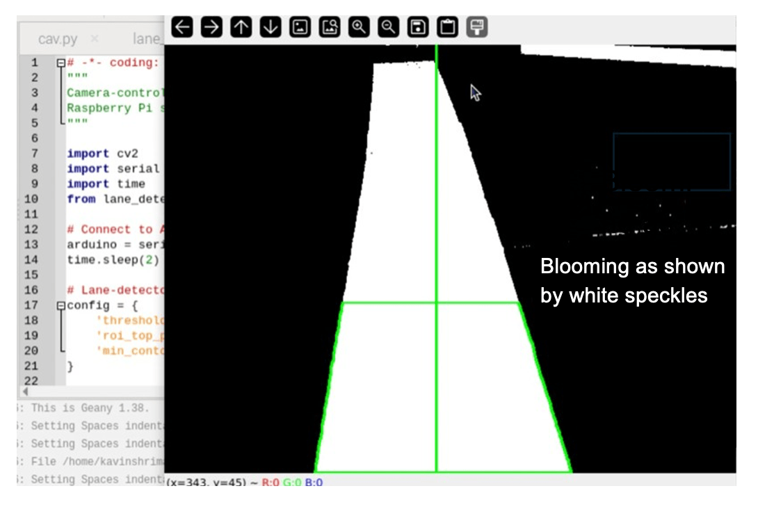
The Saturation and Blooming (533.33 Lux) At the maximum intensity of 533.33 lux, the sensor reached closer to its Full Well Capacity (FWC). As the photodiodes approached their maximum electron-holding capacity, the resulting pixel blooming caused excess charge to leak into adjacent pixels, artificially blurring the high-contrast boundary of the path as indicated in Figure 320.
This led to the peak average RMSE of 2.83 cm. Crucially, the Standard Deviation nearly doubled to 0.29 cm, indicating that the high-intensity light created a “shimmering” edge that the software could not consistently localize. An Independent Samples t-test revealed this degradation to be statistically significant (t(18) =3.77, p=0.001), as indicated in Table 2. A p<0.05, the study rejected the null hypothesis, confirming that the loss of mechanical precision and the surge in navigation jitter were deterministic outcomes of photodiode saturation.
All experimental conditions yielded statistically significant p-values when compared to the control, as indicated in Table 2, showing that the robot’s mechanical precision was non-linearly related to illuminance, with performance degrading at the electronic noise floor (0 lux), shifting at intermediate ranges (213.33 lux), and becoming highly unstable at the saturation ceiling (533.33 lux).
| Light Intensity | Avg. RMSE (cm) | Avg. SD (Jitter) | t-test (p-value) | Status | Dominant Noise Mechanism |
| 0 Lux | N/A | N/A | p<0.001 | System Failure | Read Noise Floor: The signal was entirely consumed by internal electronic interference, preventing system initialization. |
| 53.33 Lux (Control) | 2.44 | 0.15 | Reference | Optimal | Optimal SNR: Operating in the linear dynamic range allowed for maximum deterministic consistency across all 10 trials. |
| 213.33 Lux | 2.76 | 0.16 | t= 4.60 p=0.0002 | Stable (Insignificant Statistically but beginning of shot noise induced degradation) | PRNU/Shot Noise: Increased photon flux introduced minor spatial noise, causing slight navigation jitter on soft turns. |
| 533.33 Lux | 2.83 | 0.29 | T = 3.77 p=0.0014 | Significant Degradation | FWC Saturation: Pixel blooming blurred the 4.4 cm tape edges, resulting in a statistically significant loss of stability and accuracy. |
CMOS Noise Mechanisms and Path Fidelity
The data further revealed a relationship between specific CMOS noise mechanisms and the resulting mechanical performance of the mobile robot. At the 0-lux baseline, the dominance of the Read Noise floor created a total signal vacuum, rendering the 44 cm path invisible and resulting in absolute system failure. At the 53.33-lux, the transition to nominal shot noise allowed for relatively higher data fidelity, where the sensor’s 40 dB SNR supported stable navigation across all track segments. However, as illuminance increased to 213.33 lux, the introduction of Photo Response Non-Uniformity (PRNU) manifested as lateral “navigational jitters,” specifically degrading the robot’s ability to track the straight 44 cm segments with precision. This degradation approached its peak at 533.33 lux, where FWC saturation and pixel blooming induce severe edge-blurring; this loss of data fidelity was most pronounced during the 14 cm semi-circle curves, where the system was unable to resolve a sharp boundary, resulting in maximum RMSE and instability. The relative roles of various noise factors are illustrated in Table 3.
| Light Level | Dominant Noise Factor | Mechanical Impact | Path Section Most Affected |
| 0 Lux | Read Noise Floor | Total System Failure | All Segments (Invisible) |
| 53.33 Lux | Nominal Shot Noise | Optimal Precision | All Segments (Stable) |
| 213.33 Lux | PRNU / Shot Noise | Navigational Jitters | Soft Turns / 44cm Line |
| 533.33 Lux | FWC Saturation / Blooming | High Jitter / Edge Blur | 14cm Semi-Circle / Curves |
Extrapolative Analysis of the Low-Light Regime and the Non-Linear Error Profile
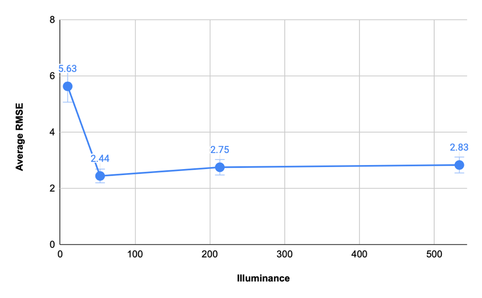
While the experimental data for the functional tiers illustrated a clear upward trend in error toward the saturation point from control, it only represented one half of the system’s performance constraints. To fully characterize the error profile, it was necessary to examine the inverse behavior as illuminance approached the physical noise floor. The theoretical lower bound, where the signal first emerges from the electronic noise floor, required an extrapolative approach to quantify the degradation of accuracy in extreme low-light conditions. While CMOS sensor performance at 10 lux, as indicated in Figure 4 and Figure 5, was not physically measured, a theoretical extrapolation using the Root-Inverse Error Law suggested a significant degradation in accuracy as illuminance approaches the sensor’s noise floor. Based on the OV2640’s 50 dB dynamic range and a calculated noise floor of 1.69 lux, the Signal-to-Noise Ratio (SNR) at 10 lux dropped to 5.92 (compared to 31.55 at the control). This 81% reduction in signal quality would likely result in a predicted RMSE of approximately 5.63 cm, representing a 130% increase in path deviation compared to the optimal photometric window. This confirmed that the non-linear error curve begins its sharpest ascent in the low-light regime, eventually resulting in the total system failure observed at 0 lux.
Conclusion and Discussion
This study into the relationship between ambient illuminance and navigational precision of CMOS sensor based robotic set-up revealed a distinct non-linear error curve, supporting the hypothesis that digital perception was dependent on an optimal photometric window: a specific range of light intensity within which a digital sensor could maintain accurate data fidelity. The findings established that while the data was highly precise under controlled illuminance, navigational precision was physically constrained by the electronic noise floor in extreme low light and Full Well Capacity (FWC) saturation in high-intensity light.
At the 53.33-lux control, the system achieved its peak performance (RMSE = 2.44 cm; SD = 0.15 cm), suggesting that within this range, the sensor could extract geometric features with maximum fidelity and minimal navigational jitter. However, as illuminance deviated toward the extremes of 0 lux and 533.33 lux, a measurable breakdown in the sensor’s ability to process spatial information was noted.
At 0 lux, the photometric window was entirely closed. In this state, the Signal-to-Noise Ratio (SNR) dropped to zero as the sensor experienced a null photon flux. The only data processed was internal electronic noise, specifically Read Noise generated within the CMOS circuitry. Because the camera required a contrast gradient to define navigation paths, the absence of a signal led to a loss of spatial coordinate precision (p<0.001).
Conversely, the performance degradation observed at 533.33 lux illustrated the physical phenomenon of photodiode saturation. As pixels reached their FWC, excess electrical charge migrated to adjacent pixels, a process known as pixel blooming. This created “optical noise” that artificially blurred the high-contrast boundaries of the 4.5 cm track, explaining the statistically significant rise in RMSE to 2.83 cm (p=0.001). Furthermore, the nearly twofold increase in Standard Deviation to 0.29 cm at this level highlighted a marked decrease in navigational stability, as the robot’s controller responded to saturation-induced artifacts.
While high-intensity light is often perceived as advantageous for computer vision, these results indicated that over-saturation is as significant a constraint on data fidelity as underexposure. This study underscored that maintaining navigational precision required a deep understanding of the stochastic nature of optical noise.
While this study established the relationship between illuminance and RMSE, it indicates several avenues for further inquiry, especially in dynamic exposure compensation algorithms in mitigating the data fidelity loss observed at the 533.33-lux ceiling. This study utilized a fixed gain, but implementing real-time High Dynamic Range (HDR) processing could theoretically flatten the ‘Non-Linear’ error curve by suppressing pixel blooming. Additionally, investigating the integration of mathematical algorithms that provides a much more accurate estimate of a system’s state such as Kalman Filtering within the signal processing pipeline may offer a method to alleviate the impact of navigation jitter induced by Read Noise in low-light environments. Further research into Model Predictive Control (MPC)21 and advanced Sensor-Fusion Based Navigation,could provide more robust path-following capabilities22,23. Finally, expanding this methodology to include variable-spectrum light sources, such as infrared or fluorescent, would determine if the deterministic outcomes of CMOS noise are wavelength-dependent, further refining the operational parameters for autonomous systems in non-controlled environments.
Reference
- Arifuzzaman, M.; Amin, S. Automated Vehicles: Are Cities Ready to Adopt AVs as the Sustainable Transport Solution? Sustainability 2025, 17, 2236. https://doi.org/10.3390/su17052236 [↩]
- L. Ravikumar, G. G. Kamat, H. N, S. T. K, and K. M. S. Autonomous vehicle navigation methods in dynamic environments: A review. Int. J. Res. Trends Innov. Vol. 7, No. 10, pp. 780-786, 2022. [Online]. Available: https://ijrti.org/papers/IJRTI2210107.pdf [Accessed: May 1, 2026] [↩]
- Yeap, K. H., & Nisar, H. (2018). Introductory Chapter: Complementary Metal Oxide Semiconductor (CMOS). In Complementary Metal Oxide Semiconductor. InTech. https://doi.org/10.5772/intechopen.73145 [↩]
- K. D. Stefanov. CMOS Image Sensors. Bristol, UK: IOP Publishing, 2022. https://doi.org/10.1088/978-0-7503-3235-4 [↩]
- G. C. Holst and T. S. Lomheim. CMOS/CCD Sensors and Camera Systems. 5th ed. Winter Park, FL: JCD Publishing, 2011 [↩]
- R. Szeliski. Computer Vision: Algorithms and Applications. 2nd ed. Springer, 2022 [↩]
- S. Feruglio, et al. Noise characterization of CMOS image sensors. Proc. 10th WSEAS Int. Conf. Circuits. pp. 102–107, 2006. [Online]. Available: https://www.academia.edu/15723242/Noise_characterization_of_CMOS_image_sensors [Accessed: May 1, 2026] [↩]
- E. S. Pereira. “Determining the Fixed Pattern Noise of a CMOS Sensor: Improving the Autonomous Star Tracker’s Sensibility.” J. Aerosp. Technol. Manag., vol. 5, no. 2, pp. 217-222, 2013. https://doi.org/10.5028/jatm.v5i2.206 [↩]
- Y. Wang, B. Wan, G. Fu, and Y. Su. “PRNU Estimation of Linear CMOS Image Sensors That Allows Nonuniform Illumination.” IEEE Trans. Instrum. Meas., vol. 70, Art. no. 5011711, pp. 1-11, 2021. https://doi.org/10.1109/TIM.2021.3088484 [↩]
- P. Zhao, B. Li, H. Zhao, W. Wen, W. Gao, and X. Fan. “Sensor-physics-driven noise modeling for low-light imaging using adversarial learning.” Appl. Sci., vol. 16, no. 6, Art. no. 2948, 2026. https://doi.org/10.3390/app16062948 [↩]
- P. I. Corke. Robotics, Vision and Control: Fundamental Algorithms in MATLAB. Berlin, Germany: Springer, 2011 [↩]
- R. Siegwart, et al. Introduction to Autonomous Mobile Robots. 2nd ed. MIT Press, 2011 [↩]
- P. I. Corke. Robotics, Vision and Control: Fundamental Algorithms in MATLAB. Berlin, Germany: Springer, 2011 [↩]
- J. T. Li. “Effect of light source on the sorting performance of a vision-based robot system.” M.S. thesis, Dept. of Industrial Technology, University of Northern Iowa, Cedar Falls, IA, 1996. [Online]. Available: https://scholarworks.uni.edu/etd/912 [Accessed: May 1, 2026] [↩] [↩]
- G. James, et al. An Introduction to Statistical Learning. 2nd ed. Springer, 2023 [↩]
- K. Brata, N. Funabiki, P. Riyantoko, Y. Panduman, M. Mentari. Performance investigations of VSLAM and Google Street view integration in outdoor location-based augmented reality under various lighting conditions. Electronics. Vol. 13, pg. 2930, 2024. https://doi.org/10.3390/electronics13152930 [↩]
- H. M. A. M. Abdelaal, C. Tee, and M. K. O. Goh. Robust Lane Detection under Varying Lighting Conditions Using Adaptive Vision-Based Techniques. J. Informatics Web Eng. Vol. 4, No. 3, pp. 336-355, 2025. DOI:10.33093/jiwe.2025.4.3.20 [↩] [↩]
- Matos F, Durães J, Cunha J. Simulating the Effects of Sensor Failures on Autonomous Vehicles for Safety Evaluation. Informatics. 2025; 12(3):94. https://doi.org/10.3390/informatics12030094 [↩]
- J. Feng, et al. Influence of noise in computer-vision-based measurements on parameter identification in structural dynamics. Sensors. Vol. 23, pg. 291, 2023. https://doi.org/10.3390/s23010291 [↩]
- M. Jarosz and B. Sniezynski. Personalization of Robot Behavior Using Approach Based on Model Predictive Control. Appl. Sci. Vol. 14, No. 24, Art. no. 11805, 2024. https://doi.org/10.3390/app142411805 [↩]
- V. Usinskis, M. Nowicki, A. Dzedzickis, and V. Bučinskas. “Sensor-Fusion Based Navigation for Autonomous Mobile Robot.” Sensors, vol. 25, no. 4, Art. no. 1248, 2025. https://doi.org/10.3390/s25041248 [↩]
- H. L. Zhang, et al. “Robust vehicle pose estimation through multi-sensor fusion of camera, IMU, and GPS.” Applied Sciences, vol. 15, no. 22, Art. no. 11863, 2025. https://doi.org/10.3390/app152211863 [↩]
- T. Zhao, W. Chen, X. Li, and R. Kang. “Reliability modelling and assessment of CMOS image sensor under radiation environment.” Chin. J. Aeronaut., vol. 37, no. 9, pp. 297–311, 2024. https://doi.org/10.1016/j.cja.2023.11.025 [↩]


