GIS-Based Graph Modeling of Pedestrian Route Safety in Pleasanton, California

Abstract

Perceptions of pedestrian safety and walkability are critically influenced by the walking environment. However, most navigation tools only optimize for distance and travel time, overlooking environmental factors can impact pedestrians’ perceived safety and comfort when walking on a route. To address this discrepancy, this study identifies safer walking routes in the Pleasanton downtown and adjacent areas. Safer walking routes are compared to the shortest possible walking routes and evaluated whether incorporating safety factors into routing models leads to meaningful changes. Route safety was quantified using five factors: streetlight density, crime rate, surface quality, proximity to buildings, and time of day. The relative importance of these factors and preferred walking distance were ranked in a public survey by 100 Pleasanton residents. These responses were normalized and converted into weights for pathfinding algorithms. Using weights based on survey responses provides a way to translate subjective perceptions of pedestrian safety into numerical weights for the routing algorithm. Dijkstra’s algorithm was used to compute the safest and shortest routes, with the safest routes being weighted using survey data. These routes were visualized using Geographic Information System (GIS) along with streetlight locations, crime density, building proximity, and road network. Results suggest that incorporating perceived safety factors can change the recommended route compared to the shortest route. This study demonstrates how pedestrian safety preferences can be incorporated into routing algorithms, using the Pleasanton downtown area as a proof-of-concept to test the method and explore their potential value for local community.

Keywords: Graph-based modeling, Pedestrian safety, Urban network modeling, Dijkstra algorithm, Multi-criteria decision analysis, Geographic information system

Introduction

Walking is an essential form of transportation in small and medium-sized cities like Pleasanton, California. Safety is often a critical factor in determining if a pedestrian feels comfortable walking in an area¹. Prior research has concluded that many factors, such as streetlight density², crime rate³, surface quality⁴, proximity to buildings⁵, and time of day⁶, can strongly influence walkability and safety levels for pedestrians. However, online navigation systems typically use shortest path algorithms like Dijkstra’s algorithm⁷ to generate routes based on distance.

Despite these findings, few studies account for multiple safety factors in creating pedestrian navigation models. Kweon et al. (2021) and Venerandi et al. (2024) highlight this gap in urban planning and pedestrian safety research, noting that current studies overlook subjective perceptions of safety to pedestrians^1,8. This study addresses the lack of pedestrian navigation services that incorporate multiple safety factors and the limited representation for perceived safety by using survey data to quantify how pedestrians prioritize different safety factors when constructing the model. Specific objectives of this research include collecting data from local pedestrians about their safety preferences, developing a balanced weighting scheme between distance and route safety using survey data, and using the weights to compare the safety-optimized route and the shortest path route.

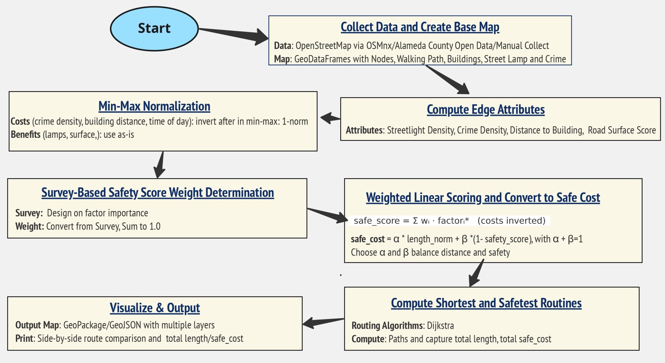
To accomplish these objectives, this study uses graph modeling and Geographic Information System (GIS) spatial visualization to analyze pedestrian routes. The base network and other features of the model were from open source data^9,10,11,12, Quantum Geographic Information System (QGIS)¹³, and NetworkX¹⁴. Each route segment is assigned a combined safety score derived from survey results and converted into a cost value. The cost value is then used to guide the shortest path algorithms into creating a safety-optimized route. The generated safety-optimized routes are compared with the traditional shortest distance routes and evaluated based on safety and efficiency. By developing an interpretable GIS model, this study aims to investigate whether incorporating perceived safety factors changes recommended pedestrian routes compared to distance optimized routes.

The scope of this study is limited to Pleasanton downtown and adjacent areas, California, and focuses on incorporating multiple safety factors that also account for perceived pedestrian safety. Limitations primarily include data-related issues such as incomplete crime records and manual collection of streetlight data. Future studies may help improve the accuracy of the model by incorporating real-time data, such as police reports or crowd-sourced safety ratings, and by collecting even more data to estimate the density of streetlights. Other researchers could also include additional factors like foot traffic volume, pedestrian traffic signals, or car traffic density in the area.

Literature Review

Prior research shows that several environmental factors influence how safe pedestrians feel while walking. Better streetlight quality has been linked to higher perceived safety and visual comfort, especially at night². Higher levels of violent crime are associated with reduced walking activity, suggesting that crime exposure lowers perceived safety³. Improvements in pavement condition and walking infrastructure have been found to enhance pedestrians’ sense of safety ⁴. Built environment features, including building presence and neighborhood structure, also shape perceived safety through both physical design and social activity⁵. In addition, time of day affects route choice and behavior, with nighttime conditions leading to different safety perceptions compared to daytime settings⁶.

Other studies have created models to address problems such as traffic safety, urban design, and pedestrian navigation. For example, some research has estimated pedestrian safety using street road classification and crossing type to characterize risk at the network level¹⁵. Other urban safety models in previous studies, such as SafeRoute (Levy et al., 2020)¹⁶ and SafePaths (Galburn et al. 2016)¹⁷, focus mainly on avoiding high-crime segments and do not consider other environmental factors that could also affect pedestrian safety perceptions. Many of these existing tools also do not incorporate lighting conditions, crime density, sidewalk surface quality, or proximity to buildings into a single model.

Methods

Study Area

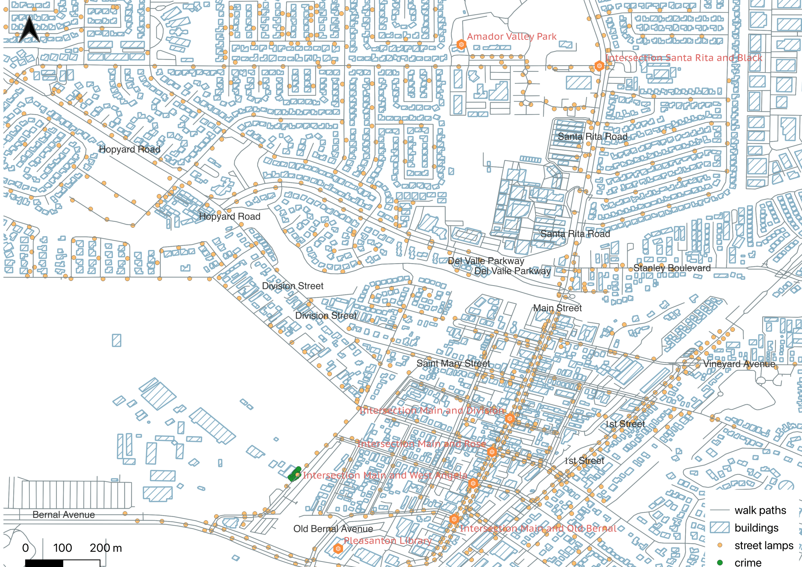
The study uses the one mile corridor between Pleasanton Library and the intersection between Main Street and Angela Street as a base case. A second longer route was constructed within the adjacent downtown area to examine the impact of the safety weights on a longer route with different environmental conditions. Pleasanton downtown is also one of the most frequently used walking areas in Pleasanton, CA. According to our public survey, 77% of participants indicated that they walked in the area either “sometimes” or “often”. Furthermore, some of the most frequently visited civic and recreational destinations, including the Civic Center and local parks, are connected by this corridor. These key features make Pleasanton downtown an ideal location to study pedestrian safety.

Data Sources

This study used open-source and municipal data about the Pleasanton downtown and adjacent areas. Data for the road network of Pleasanton downtown and pedestrian accessible walkways were collected from OpenStreetMap (OSM)⁹. These walkways were restricted to roads with sidewalks and were mapped using GIS to form a base network. Data about crime in the Pleasanton downtown area was collected through the Alameda County Open Data Hub^10,11 and later used for calculating the amount of crime in the area. Due to the limited data available, streetlight data was manually collected or observed from satellite imagery¹². In January 2026, a new version of Google Earth Professional¹⁸was released that allowed for the identification of infrastructure, including streetlights. The manually digitized data was then cross checked with this updated imagery to correct any possible errors. Additional streetlight information was added where available. Sample manual field checks were also conducted to confirm the accuracy of selected locations.

Layer	Source	Description/Construction Method
Buildings	OpenStreetMap9 via OpenStreetMap NetworkX(OSMnx)19	Calculated using distance to nearest building centroid
Footway	OpenStreetMap9 via OSMnx19	Identified walkable paths from OpenStreetMap footway data, including information about surface condition.
Crime incidents	Alameda County Open Data Hub (ALCO)10, 11	Mapped incidents from the “Crime Reports 2012-July 2022”10dataset and the “Crime Reports July 2022-Present”11 dataset
Streetlamp (partial manual)	Manually digitized from Google Maps12 reference OpenStreetMap9 via OSMnx19 Google Earth Professional 202618	Plotted streetlight locations from Google Maps12, Google Earth18 or obtained from OpenStreetMap9.  Streetlights within 100 meters of each road segment were linked to the corresponding segment.

Pedestrian Network Construction in GIS

The pedestrian network was constructed in QGIS¹³ by integrating the road network with different layers representing walkable route segments, streetlights, crime incidents, and building locations (Table 2). The surrounding area of each road segment, which represents the available pedestrian accessible area, was defined. Information such as streetlights, crime locations, and nearby buildings within this area was then assigned to the corresponding road segment. Sidewalk quality was categorized using numerical scores to quantify the quality of a surface. These attributes were normalized to produce a safety score for each road segment, which was then converted into a safety cost and used by routing algorithms.

To define this surrounding pedestrian area more precisely, different spatial rules were applied for each safety factor. Streetlight density was calculated using a symmetric 100 m (0.06 mi) GIS buffer around each road segment. Crime exposure was measured using a larger 1000 m (0.62 mi) buffer as base, following a sensitivity analysis comparing multiple crime buffer sizes and their impact on routing results, a 500 m (0.31 mi) radius was selected as the final setting (see “Crime Buffer Sensitivity Analysis” below for details). Building influence was represented by the minimum distance from each road segment to the nearest building, while surface quality was taken directly from road attributes without buffering. Buffers from nearby streets were allowed to overlap, and each segment was scored independently. Dead-end streets and cul-de-sacs were retained in the network and scored in the same way as other segments but were only selected if they formed a complete path between the origin and destination. Disconnected segments were excluded implicitly, as routing was performed only on the connected component containing two endpoints.

Component of GIS Network	Component Attributes	Data Source	Purpose in Network
Study Area	Pleasanton Downtown Surrounding Area Latitude: 37.6530 to 37.7050 Longitude: -121.9180 to -121.8500	Defined manually using QGIS13 map	Boundary layer used to limit all data to the study area.
Start Point (Based Route)	Pleasanton Library Latitude:  37.657154 Longitude: -121.881429	Manual coordinate selection in QGIS13	Used as base route origin node for routing
End Point (Based Route)	Intersection of Main Street and Angela Street Latitude:  37.659448 Longitude: -121.876571	Manual coordinate selection in QGIS13	Used as base route destination node for routing
Start Point (Longer Route)	Amador Valley Park Latitude:  37.672195 Longitude: -121.877248	Manual coordinate selection in QGIS13	Used as longer route origin node for routing
End Point (Longer Route)	Intersection of Peters Avenue and Angela Street Latitude:  37.659924 Longitude: -121.877529	Manual coordinate selection in QGIS13	Used as longer route destination node for routing
Street Network	Created using pedestrian-accessible street and path segments	OpenStreetMap9	Converted into network edges for routing
Intersections and Nodes	Intersections and endpoints of streets and paths	Derived from street network topology	Used as network nodes in pedestrian graph
Streetlight Locations	Geographic coordinates of public streetlights	Manually digitized Google Maps 12Google Earth 18 OpenStreetMap9	Manual creating streetlamp layer, used to compute lighting density per segment
Crime Incident Points	Locations of reported police or public safety occurrences	Alameda County Open Data Hub10,11	Manual creating crime layer, used to compute crime proximity score
Sidewalk Surface	Categorizes road segments into surface types	OpenStreetMap9	Used to classify the condition of sidewalks along each segment
Time of Day	Numerical parameter representing day (1) and night (0) conditions	Manually defined parameter	Adjusts safety score weighting in daytime or nighttime conditions

Survey Design

An anonymous, public survey completed by 100 Pleasanton residents was used to gather contextualizing information and determine the importance of each safety factor: streetlights, crime, surface condition, proximity to buildings, and time of day (day vs. night). This survey was approved by the Alameda County Institutional Review Board. It also was conducted anonymously and with online consent from all participants in accordance with IRB requirements and ethical research guidelines²⁰. Participants indicated whether they were an adult or minor and their gender when completing the survey. Survey data was stored securely in password-protected files. The survey was split into three sections, each addressing a different aspect of pedestrian safety.

The first section addressed the frequency of visits and common routes in the Pleasanton downtown area. This information helped confirm that the study corridor was a regularly used route by local pedestrians. About 77% of the participants indicated that they either “sometimes” or “often” walked in the area. When asking survey respondents about their walking routine, the highest percentage of participants (28%) reported walking along the exact route analyzed in this study while other participants reported walking along similar routes nearby. These results suggest that the study area represents typical pedestrian traffic in Pleasanton downtown.

The second section asked participants to indicate the impact of each safety factor and to rank them according to their perceived impact on safety. The weights of each safety factor were then adjusted according to participant responses. Participants ranked time of day as the most important factor and proximity to buildings as the least important. These rankings partially aligned with our hypothesis. Crime remained one of the most highly weighted factors, but it was not the strongest factor after the survey. Instead, time of day received the highest weight in both daytime and nighttime settings. Proximity to buildings, which was expected to be the least important, received a higher weight than predicted.

The final section asked the participants how much additional distance they would be willing to walk for a safer route. This was to ensure the safe route calculated by our model would remain practical for walking and not excessively long. Responses were then converted into weights, where willingness to walk reduced the weight of route length.

A Friedman test was used to evaluate whether differences in perceived importance across factors were statistically significant. Mean importance scores and standard deviations were computed to quantify uncertainty.

To investigate the difference between the least and most important factors, a numerical ranking system was applied to the survey data. Each “most important” selection was assigned 5 points, and each “least important” selection was assigned 1 point. The points were then summed across all survey responses. The point system was then translated into the weighting scheme.

Safety Score and Safety Cost

Safety Score Calculation with Weighted Linear Scoring

Weighted Linear Scoring was used to calculate the safety score of each path. A higher safety score indicated a safer road segment, while a lower safety score indicated an unsafe road segment. The weighting and scoring procedure consisted of the following steps. Weights were first assigned to five factors: streetlights, crime, surface condition, distance from buildings, and time of day. These factors were then split into two weight sets (Day vs Night). The purpose of this split was to compare the effect of the same factors on perceived safety, since nighttime pedestrian priorities differed from daytime pedestrian priorities ⁶. This difference can be attributed to the increased influence of various factors such as lighting and the lack of open space⁶. The limited open space factor described by Filomena and Wozniak (2025) corresponds to the proximity to buildings factor considered in this study, both reflecting the influence of environmental factors on perceived safety⁶.

The time of day variable is the same for all road segments within a given scenario. When time of day indicates daytime, the streetlight factor receives zero weight because artificial lighting is not used during daytime. When the variable indicates nighttime, the streetlight factor is assigned a positive weight to demonstrate greater importance. Time of day is included both as a binary indicator and through separate weight sets because it defines the scenario and adjusts how strongly other safety factors influence the overall safety score.

After the weights were assigned, each factor was then labeled as a beneficial factor or a cost factor. Beneficial factors increased perceived pedestrian safety as the factor increased. To illustrate, factors such as increased streetlight density and higher sidewalk quality were labeled as beneficial and increased the safety score. Cost factors decreased perceived safety as the value increased and included factors such as high crime or distance from buildings. These factors were then normalized on a scale of 0 to 1 to allow for comparability. The normalized cost factors were also inverted by being subtracted from 1 to ensure that a high safety score would indicate higher safety. The cost factors are meant to decrease as the safety score increases, since they influence pedestrian safety perception negatively. This inversion ensures that all factors align on a common scale where higher values represent safer routes.

Safety Score Formula with 5 Factors:

(1)  

Variables:

SL(e) = streetlight density (beneficial factor)
CR(e) = crime intensity (cost factor)
SQ(e) = sidewalk surface quality (beneficial factor)
PB(e) = proximity to buildings (cost factor)
TD(e) = time of day exposure factor (cost factor)

Normalize each factor to 0-1:

(2)  

Weights:

(3)  

Initial Safety Factor Hypothesis

The initial hypothesis was based on previous research about the impact of various environmental factors on perceived safety ^1,4,5. Each weight set was normalized to sum to 100%. In the daytime model, crime rate was weighted to be highest at 40%, as nearby crime remains a significant safety concern regardless of time since crime can still occur during the day^{3, 10,11}. Time of day and sidewalk quality were ranked the next highest at 30% and 20%, respectively. Time of day was weighted at 30% because it shows whether it is day or night and determines whether streetlights should matter more at night or less during the day in the safety calculation^6,. Sidewalk quality can be an indicator of the quality of the surrounding urban environment^4,8. However, it was weighted lower than time of day because it has less direct influence on perceived safety during daytime¹. The lowest weighted factors were proximity to buildings and streetlight density the lowest, rated at 10% and 0% respectively⁸. Proximity to buildings was weighted at 10% because its influence on perceived safety is low during the day, when visibility is high⁶. Streetlights are not used during the day and therefore were weighted at 0.

In the nighttime model, streetlight density and nearby crime were assigned the highest weights at 30% each. These two factors were rated the same because they have been shown to have a strong positive correlation with feelings of safety^2,3,4. Time of day was assigned a weight of 20%, reflecting prior research⁶. Proximity to buildings and sidewalk quality received the lowest weight (10%) as these factors demonstrated weaker associations with perceived safety^1,5.

How the Survey Adjusted the Safety Factor Weights

In order to identify which safety factors were most important, survey respondents ranked safety factors from most to least important. These responses were then converted into points (5 = most important, 1 = least) and normalized to show how much weight each safety factor holds relative to the others. In addition to the ranking, participants rated the importance of each factor on a scale of 1-7. When two or more factors received similar point totals, the individual importance rankings were used to determine whether the factors should be adjusted to have the same weight or different weights.

Safety Cost Calculation

To account for both distance and safety simultaneously, the final model was weighted using both distance and safety cost. A safety score for each road segment was first calculated using the method outlined in this study. The routing algorithms used in this study operate on weighted graphs and require a cost value on each edge to compute the optimal route⁷. These algorithms select the road segments with the lowest assigned cost values and compute the optimal route by minimizing the total cost of the route. Therefore, to integrate the safety score into these algorithms, it was converted into a cost value called safety cost. The calculation of safety cost is as follows:

(4)  

Where:

α = weight of distance

β = weight of safety score

1 – safety score = converts high safety to a low cost

To determine how much distance influences the safety cost calculation, participants were asked how much further they were willing to walk on a 1-mile route. Options were grouped into distance ranges, and each range was assigned a corresponding distance-weight value. For example: little willingness to walk further corresponded to high distance weight and high willingness to walk further corresponded to lower distance weight. Most participants chose an option within the range of 0.1-0.7 miles. The average of the survey responses was then determined to be the final distance weight (alpha). The final weight distance and the safety score were used to calculate the safety cost.

(5)  

To calculate this average more precisely, the survey responses were converted into predefined distance-weight percentages. Each distance category was assigned a specific length weight: 0 miles (0 m) = 100%, 0.1-0.2 miles (160.93-321.87 m) = 80%, 0.2-0.3 miles (321.78-482.80 m) = 70%, 0.3-0.5 miles (482.80-804.67 m) = 50%, 0.5-0.7 miles (804.67-1126.54 m) = 30%, and “Other” = 0%. A weighted average was then computed by multiplying each percentage by the number of responses in that category and dividing by the total number of respondents. This value defined the final distance weight (α), and the safety weight was calculated as β = 1 − α.

Crime Buffer Sensitivity Analysis

To evaluate the robustness of the crime factor, a sensitivity analysis was conducted by varying the buffer radius used to calculate crime exposure. The initial model applied a 1000 m buffer around each road segment to represent neighborhood-level crime conditions. Additional analyses were performed using smaller buffer sizes of 100 m (0.06 mi), 300 m (0.19 mi), and 500 m (0.31mi) to examine how buffer choice influences safety costs and routing results. For each buffer size, the route length and total safety cost were recalculated for both the shortest and safest routes.

Literature-Based Weighting Schemes

In addition to the survey-based weights, alternative weighting schemes were developed based on findings from prior research on perceived pedestrian safety. Previous studies do not provide exact numerical weights but consistently highlight the relative importance of certain factors under different conditions. Based on these patterns, two literature weighting schemes were constructed. The first scheme emphasized the importance of visibility factors, including streetlights and time of day. The second scheme placed greater emphasis on built environment and infrastructure factors, such as surface quality and proximity to buildings (see Table 3 for values). The adjusted weights were modified from the survey baseline to reflect these priorities.

A sensitivity test was conducted to evaluate the effect of these alternative weight sets. For each weighting scheme, route length and safety cost values were recalculated, and analysis was repeated. The shortest and safest routes were then compared across the baseline and literature-based models to assess whether route selection changed.

Test Set	Time of Day	Streetlights	Crime	Sidewalk Surface	Buildings	Day/Night Weight
Baseline (survey-based)	Day	0	0.25	0.22	0.18	0.35
	Night	0.2	0.2	0.17	0.13	0.3
Scheme A: visibility & time emphasis	Day	0	0.2	0.2	0.25	0.35
	Night	0.3	0.2	0.15	0.1	0.25
Scheme B: built environment & infrastructure emphasis	Day	0	0.18	0.27	0.35	0.20
	Night	0.20	0.18	0.22	0.30	0.1

Graph-Based Routing Algorithms and Model Workflow

The road network of the associated area of Pleasanton, California was modeled as a graph. Nodes on the graph corresponded to street intersections and edges represented individual road segments. This graph structure served as the foundation for visualizing safety attributes and computing weighted safety cost values. Dijkstra’s algorithm⁷ created routes along this framework using the safety cost values. These routes were also displayed on the GIS system and compared visually using the safety cost and distance metrics.

Results

Survey Findings

The survey was completed by 100 Pleasanton residents who were 99% adults and 1% minors. Gender information was also collected with a 54% male and 46% female distribution. The following survey results illustrate how respondents rank safety factors in terms of perceived importance.

Survey Question: When thinking about walking safety, which of these factors is the most important and the least important to you? (Most = 5 points, 2nd = 4 points, 3rd = 3 points, 4th = 2 points, least =1 point)

Safety Factor	Total Points
Streetlight Density	342
Crime Rate	341
Sidewalk Surface Quality	265
Proximity to Buildings	267
Time of Day	401

Survey responses showed clear differences in perceived importance among safety factors (Table 5). The Friedman test indicated that these differences were statistically significant (χ² =  61.2558, p < 0.001), suggesting that the observed ranking is unlikely because of random variation. Time of day received the highest average importance score, followed by streetlight density and nearby crime.

Safety Factor	Mean Score	Standard Deviation
Streetlight Density	3.42	1.26
Crime Rate	3.41	1.37
Sidewalk Surface Quality	2.65	1.39
Proximity to Buildings	2.67	1.29
Time of Day	4.01	1.06

In the case of the number of streetlights and nearby crime, the two factors only differed by one point in the ranking question. When looking at the factors individually, 76% found good street lighting to be very important and 72% found few crimes nearby to be very important. The difference between the two factors’ importance when evaluated alone was small enough not to significantly affect their proportional weights. However, in the case of sidewalk quality versus proximity to buildings, 61% found sidewalk quality to be very important while only 48% found proximity to buildings very important. This difference was large enough to have an impact on the ratio of the final weights, resulting in a higher weight for sidewalk quality in the final model.

Participants were also asked to indicate the relative importance of safety compared to distance when selecting their walking routes.

Survey Question: How many more miles would you be willing to walk beyond a 1 mile route if it meant choosing a safer route?

Extra Distance Willing to Walk	Participant Selections
0 miles (0 m)	5
0.1-0.2miles (160.93-321.87 m)	20
0.2-0.3miles (321.78-482.80 m)	29
0.3-0.5miles (482.80-804.67 m)	22
0.5-0.7miles (804.67-1126.54 m)	22
Other	2

The distance weight was calculated to be approximately 60%. Safety weight then accounted for 40% in the final routing decision. This suggests that while route distance remains an important factor, participants also value safety when choosing their walking routes.

Safety Factor Weights from Public Survey

Survey responses were converted into weighting schemes for both daytime and nighttime conditions. During the day, as shown in Table 7, time of day and nearby crime had the two highest weights. In the “Day Weights (Before Survey)” column, crime was 40% and time of day was 30%, while in the “Day Weights (After Survey)” column, time of day increased to 35% and crime decreased to 25%. This difference indicates that time of day was viewed as significantly more important to perceived safety. At night, as shown in Table 7, time of day was still a key factor. Its weight increased from 20% in the “Night Weights (Before Survey)” column to 30% in the “Night Weights (After Survey)” column. Streetlight density and crime, which were both 30% before the survey, decreased to 20% after the survey and were now equally influential, indicating that factors affecting perceptive safety shift according to environmental conditions such as time.

These patterns also suggest that Pleasanton residents are especially attentive to changes in visibility and the presence of potential crime risks when assessing route safety. Small-scale improvements, such as adding or repairing streetlights and maintaining clear sightlines, could increase comfort for pedestrians walking in Pleasanton downtown.

Safety Factor	Normalization	Direction	Day Weights (Before Survey)	Day Weights (After Survey)	Night Weights (Before Survey)	Night Weights (After Survey)
Streetlights	Lamp count within ~100 m buffer	Benefit	0	0	0.30	0.20
Crime	Crime incidents within ~500 m	Cost	0.40	0.25	0.30	0.20
Sidewalk condition	Map surface to comfort score	Benefit	0.20	0.22	0.10	0.17
Proximity to buildings	Distance to nearest building	Cost	0.10	0.18	0.10	0.13
Day/Night	0 (day) or 1 (night)	Cost	0.30	0.35	0.20	0.30

Safety-Distance Trade-Off Derived from Public Survey

The distance weight and safety weight were modified according to survey responses (See Table 6). Based on the weighted average of survey response, the calculated value for α was 58.9%, which was rounded to 0.6 for model implementation. The corresponding safety weight was therefore β = 0.4. This change in distance and safety weight indicates that while route distance remains relevant, Pleasanton residents place a comparatively greater importance on safety. According to survey results, safety was calculated to contribute to 40% of the combined weights, which was 10% higher than the hypothesized weight of 30%. This outcome suggests that residents are willing to walk farther if the route is perceived as safer, as long as the added walking distance remains reasonable.

Scenario	α (Distance Weight)	β (Safety Weight)
Balanced distance and safety (Before Survey)	0.7	0.3
Balanced distance and safety (Survey Adjust)	0.6	0.4

Results of Crime Buffer Sensitivity Analysis

The crime buffer sensitivity analysis showed different levels of variation between the base and longer routes. Crime incidents in the study area were concentrated at one location. For the base’s shorter route, both 500 m (0.31 mi) and 1000 m (0.62 mi) buffers produced the same results, while 100 m (0.06 mi) and 300 m (0.19 mi) buffers often resulted in many zero crime counts. For the longer route, the 1000 m (0.62 mi) buffer spread the crime effect across a wide area and increased overall safety cost, especially at night. In contrast, the 500 m (0.31 mi) buffer captured the hotspot without spreading its effect too broadly. To balance local sensitivity and model consistency across both routes, a unified 500 m (0.31 mi) crime buffer was selected for all analyses.

Route	Crime buffer (m)	Time	Objective	Weight used	Total distance (m)	Total safety cost
Base	100 (0.06 mi)	Day	Shortest	Length	585.36 (0.36 mi)	359.61
Base	100 (0.06 mi)	Day	Safest	Length	586.00 (0.36 mi)	359.33
Base	100 (0.06 mi)	Night	Shortest	Length	585.36 (0.36 mi)	369.14
Base	100 (0.06 mi)	Night	Safest	Length	586.00 (0.36 mi)	368.16
Base	300 (0.19 mi)	Day	Shortest	Length	585.36 (0.36 mi)	360.89
Base	300 (0.19 mi)	Day	Safest	Length	586.00 (0.36 mi)	360.62
Base	300 (0.19 mi)	Night	Shortest	Length	585.36 (0.36 mi)	384.37
Base	300 (0.19 mi)	Night	Safest	Length	586.00 (0.36 mi)	383.40
Base	500 (0.31 mi)	Day	Shortest	Length	585.36 (0.36 mi)	365.30
Base	500 (0.31 mi)	Day	Safest	Length	586.00 (0.36 mi)	364.55
Base	500 (0.31 mi)	Night	Shortest	Length	585.36 (0.36 mi)	416.29
Base	500 (0.31 mi)	Night	Safest	Length	586.30 (0.36 mi)	412.35
Base	1000  (Base Buffer)	Day	Shortest	Length	585.36 (0.36 mi)	365.30
Base	1000  (0.62 mi, Base Buffer)	Day	Safest	Length	586.00 (0.36 mi)	364.55
Base	1000  (0.62 mi, Base Buffer)	Night	Shortest	Length	585.36 (0.36 mi)	416.29
Base	1000  (0.62 mi, Base Buffer)	Night	Safest	Length	586.30 (0.36 mi)	412.35
Longer	100 (0.06 mi)	Day	Shortest	Length	1937.52 (1.20 mi)	1206.23
Longer	100 (0.06 mi)	Day	Safest	Length	1970.55 (1.22 mi)	1201.04
Longer	100 (0.06 mi)	Night	Shortest	Length	1937.52 (1.20 mi)	1257.68
Longer	100 (0.06 mi)	Night	Safest	Length	1970.55 (1.22 mi)	1226.69
Longer	300 (0.19 mi)	Day	Shortest	Length	1937.52 (1.20 mi)	1206.23
Longer	300 (0.19 mi)	Day	Safest	Length	1970.55 (1.22 mi)	1201.77
Longer	300 (0.19 mi)	Night	Shortest	Length	1937.52 (1.20 mi)	1257.68
Longer	300 (0.19 mi)	Night	Safest	Length	1970.55 (1.22 mi)	1230.19
Longer	500 (0.31 mi)	Day	Shortest	Length	1937.52 (1.20 mi)	1208.31
Longer	500 (0.31 mi)	Day	Safest	Length	1940.87 (1.21 mi)	1204.87
Longer	500 (0.31 mi)	Night	Shortest	Length	1937.52 (1.20 mi)	1268.34
Longer	500 (0.31 mi)	Night	Safest	Length	1979.42 (1.23 mi)	1246.30
Longer	1000  (0.62 mi, Base Buffer)	Day	Shortest	Length	1937.52 (1.20 mi)	1220.85
Longer	1000  (0.62 mi, Base Buffer)	Day	Safest	Length	1970.55 (1.22 mi)	1211.14
Longer	1000  (0.62 mi, Base Buffer)	Night	Shortest	Length	1937.52 (1.20 mi)	1327.45
Longer	1000  (0.62 mi, Base Buffer)	Night	Safest	Length	1962.67 (1.22 mi)	1309.32

Shortest vs Safest Routes

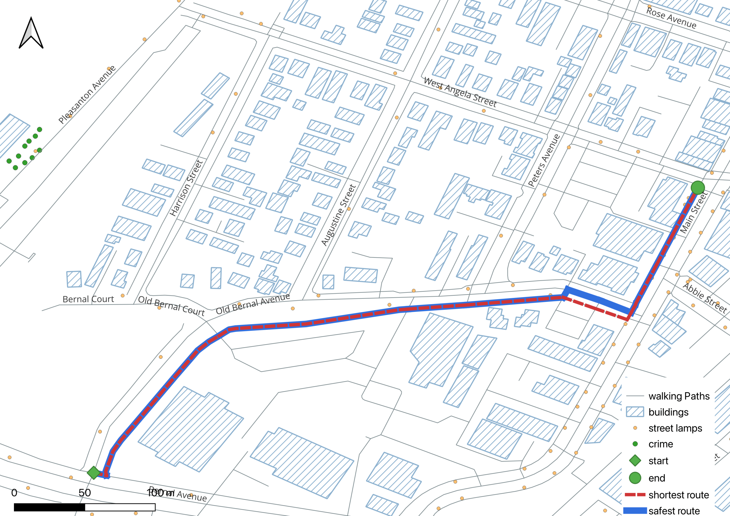
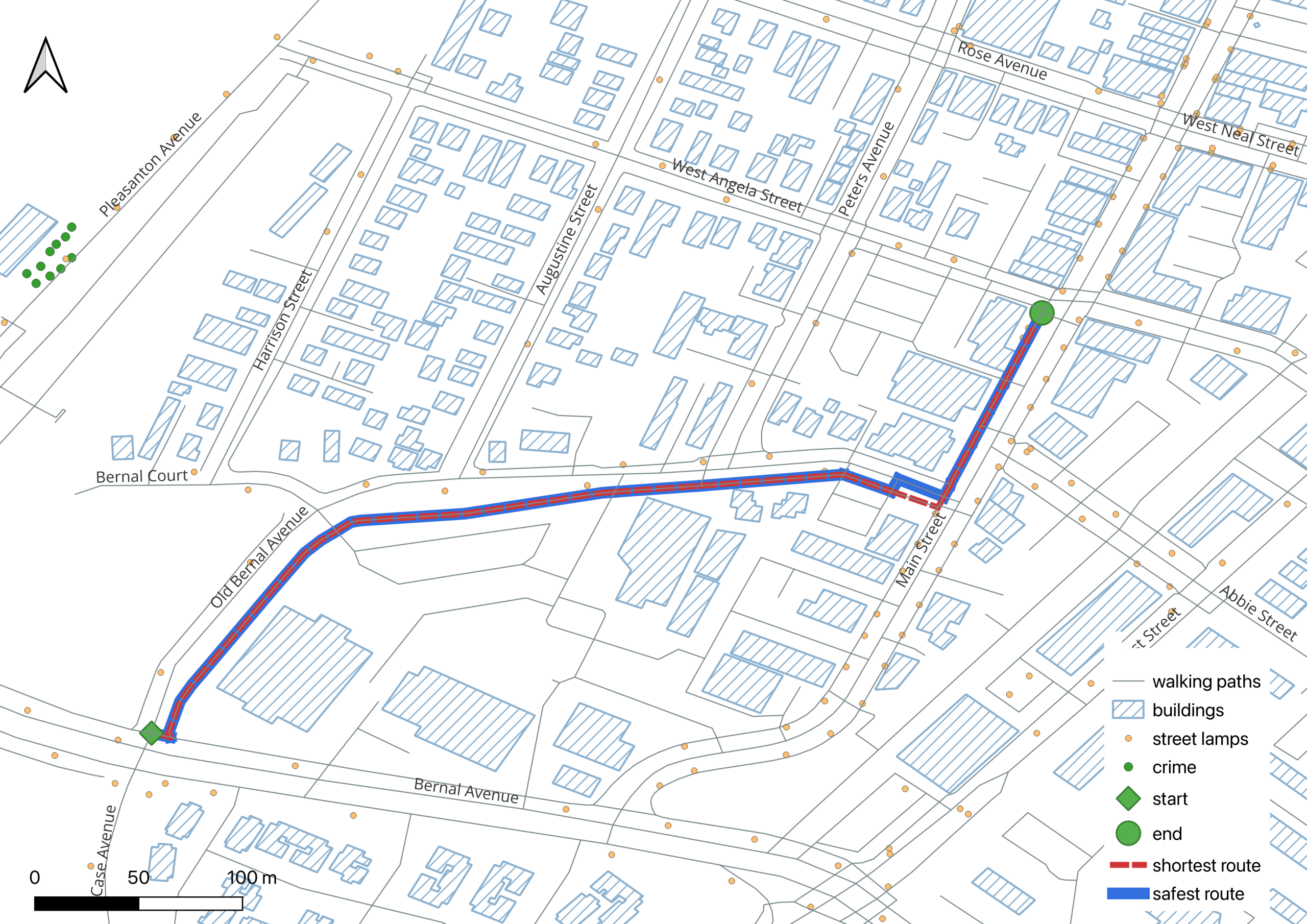
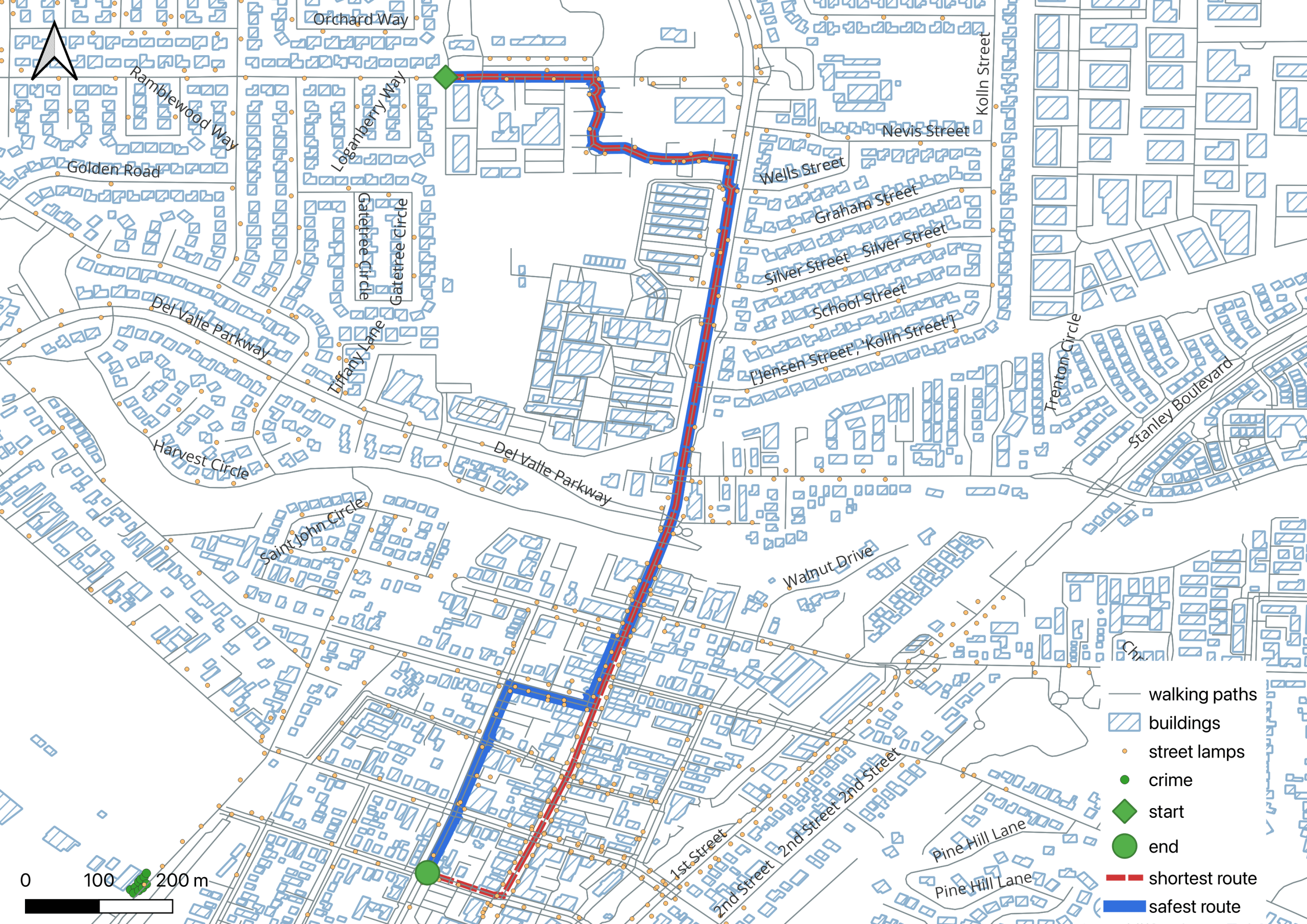
Based on the adjusted weights for the five safety factors and the overall balance between safety and walking distance, the shortest base route between Pleasanton Library and Main Street measured 585.36 meters (0.36 mi) in both daytime and nighttime conditions. After incorporating streetlight density, nearby crime, surface condition, distance from buildings, and time of day, the resulting safer base routes measured 586 meters (0.36 mi) during the day and 586.3 meters (0.36 mi) at night. The safety-optimized route was longer, it shifted toward streets with better lighting, fewer crime incidents, and safer walking conditions. However, for shorter downtown start-to-end locations, the shortest and safest routes were nearly identical in both length and alignment.

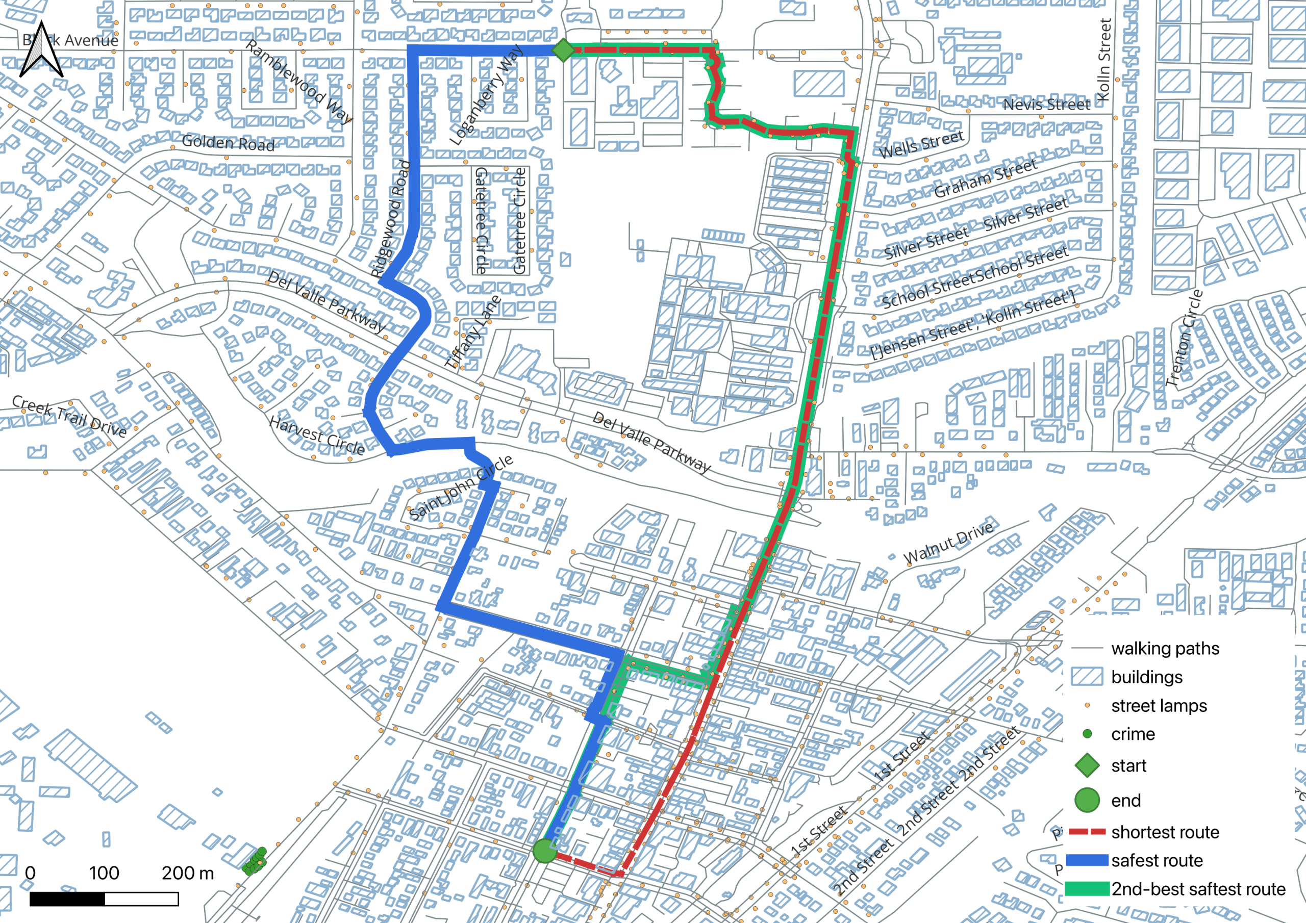
A different pattern was observed for the longer route from Amador Valley Park to central Pleasanton downtown. The shortest route measured 1937.52 meters (1.20 mi) in both daytime and nighttime conditions. During the day, the safety-optimized route measured 1940.87 meters (1.21 mi). The second-best safe route closely aligns with the safest route. It is not included in Figure 5 because the map scale does not clearly distinguish it from the primary safest route. At night, the safest route shifted to a largely different path and increased to 1979.42 meters (1.23 mi), while the second-best safe route (1947.04 m, 1.21 mi) follows a different path. The greater distance change and route shift at night indicate that safety factors, particularly lighting and time of day, had a stronger influence on route selection.

Route	Time	Objective	Weight used	Total distance (m)	Total safety cost
Base	Day	Shortest	Length	585.36 (0.36 mi)	365.30
Base	Day	Safest	Safety Cost	586.00 (0.36 mi)	364.55
Base	Night	Shortest	Length	585.36 (0.36 mi)	416.29
Base	Night	Safest	Safety Cost	586.30 (0.36 mi)	412.35
Longer	Day	Shortest	Length	1937.52 (1.20 mi)	1208.31
Longer	Day	Safest	Safety Cost	1940.87 (1.21 mi)	1204.87
Longer	Day	2nd‑best safe route	Safety Cost	1940.88 (1.21 mi)	1204.88
Longer	Night	Shortest	Length	1937.52 (1.20 mi)	1268.34
Longer	Night	Safest	Safety Cost	1979.42 (1.23 mi)	1246.30
Longer	Night	2nd‑best safe route	Safety Cost	1947.04 (1.21 mi)	1261.40

Results of Literature Based Weight Testing

The weight testing showed that route selection remained stable in many cases, while also demonstrating meaningful sensitivity under certain conditions. For the base route, the safest route did not change during daytime across all weight sets, and only one nighttime scenario (Scheme B) resulted in a route shift. For the longer route, changes occurred primarily during daytime when alternative weighting schemes were applied, and under Scheme B at night. The shortest route distance remained constant and differences in total safety cost were moderate in all cases. These findings suggest that the model remains stable when reasonable changes are made to weighting assumptions. However, it also responds appropriately when specific safety factors are weighted higher, especially in more complex routes.

Test Set	Route	Time of Day	Shortest route length (m)	Safest route length (m)	Δ length (m)	Total safe cost (safest)	Safest route changed
Baseline (survey-based)	Base	Day	585.36 (0.06 mi)	586.00 (0.06 mi)	0.64 (0.00 mi)	364.55	N
		Night	585.36 (0.06 mi)	586.30 (0.06 mi)	0.94 (0.00 mi)	412.35	N
	Longer	Day	1937.52	1940.87	3.35 (0.00 mi)	1204.87	N
		Night	1937.52	1979.42	41.90 (0.03 mi)	1246.30	N
SchemeA: visibility & time emphasis	Base	Day	585.36	586.00	0.64 (0.00 mi)	364.29	N
		Night	585.36	586.30	0.94 (0.00 mi)	395.92	N
	Longer	Day	1937.52	1970.55	33.03 (0.02 mi)	1206.84	Y
		Night	1937.52	1979.42	41.90 (0.03 mi)	1241.54	N
SchemeB: built environment &infrastructure emphasis	Base	Day	585.36	586.00	0.64 (0.00 mi)	371.75	N
		Night	585.36	586.00	0.64 (0.00 mi)	402.11	Y
	Longer	Day	1937.52	1979.42	41.90  (0.03 mi)	1217.24	Y
		Night	1937.52	1980.08	42.56 (0.03 mi)	1238.54	Y

Distribution of Safety Scores Across the Network

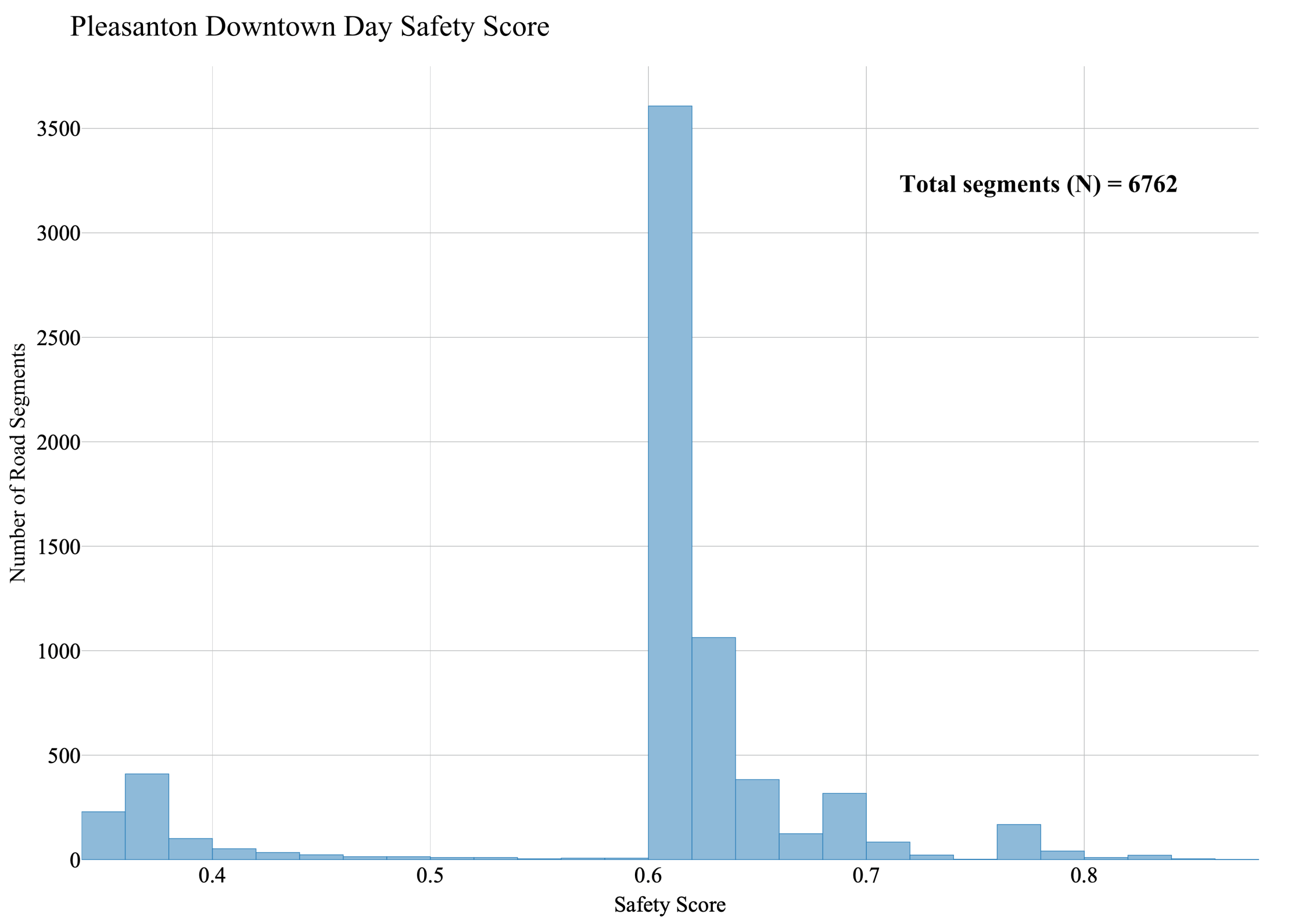
Safety score histograms revealed how safe pedestrians perceived Pleasanton downtown during daytime and nighttime.

During the day, road segment safety scores were graphed on a scale of 0 to 1. The graph had two peaks: the largest peak (over 3,500segments out of total 6762 segments) appeared at approximately 0.60, and the smaller peak (about 1,100 segments) appeared at approximately 0.62. This distribution indicates that most areas in Pleasanton downtown are perceived as moderately safe. The segments that scored lower represent locations that most respondents perceived as unsafe.

At night, safety scores shifted downward, ranging mostly from 0 to 0.5. The majority of segments (around 2000 segments out of total 6762 segments) had a score of around 0.22, followed by around 1250 segments around 0.24 which suggests that more areas were perceived as unsafe in darker conditions. A smaller portion of segments scored under 0.1, indicating that certain segments are perceived as highly unsafe at night by local pedestrians.

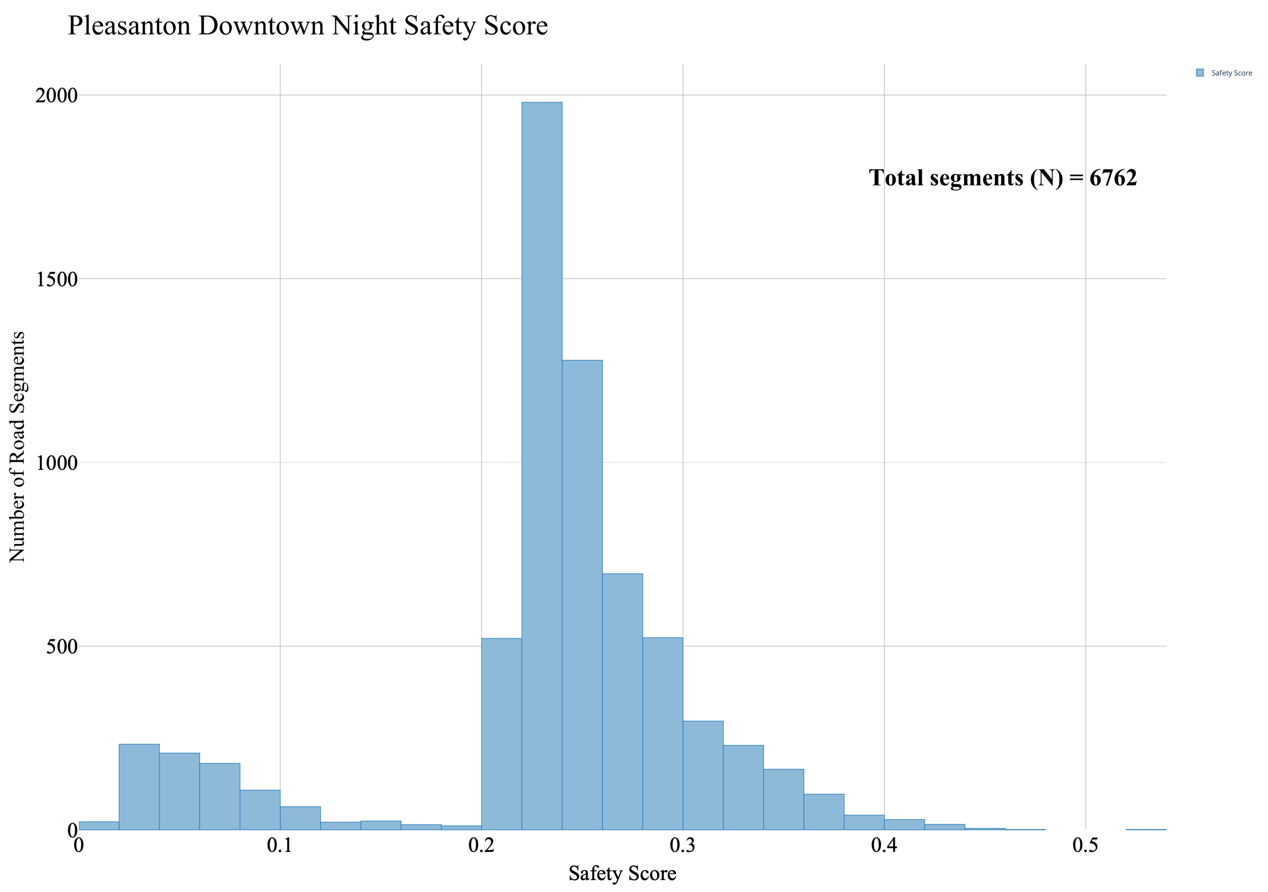
This difference between the nighttime and daytime safety scores indicates that the perceived drop in safety at night could be related to the changing importance of the safety factors. Streetlights and crime had a significantly higher influence on pedestrian safety during nighttime conditions. This suggests that this difference in safety scores is attributed to lower visibility since crime conditions remained similar.

Preliminary Route Preference Validation

To provide an initial validation of the model’s route selection, we conducted interviews with 20 Pleasanton locals who provided verbal consent (15 adult male, 5 adult female). Participants were shown the shortest route, the safest route, and the second safest route identified by the model. They were asked which route they felt safer walking on. During daytime conditions, 11 participants (8 male, 3 female) reported feeling safer on the model-selected safest route, while during nighttime conditions, 12 participants (7 male, 5 female) preferred the model-selected safest route. This indicated that the safety weights from the initial survey represented local opinion accurately. None of the participants chose the second-best safest route.

Discussion

This study demonstrates that integrating safety-related attributes can affect recommended pedestrian travel routes. When the five safety factors were considered, the resulting route avoided areas that had a low safety score. During daytime and nighttime, the safety-weighed route increased in distance and achieved a reduced safety cost.

Considering the path difference between the shortest and safest routes for both longer and shorter routes, it can be concluded that incorporating safety factors into a shortest path algorithm can make difference in route selection. In compact downtown settings with short trip distances, the optimized route closely aligns with the shortest path. However, for longer trips and under higher-risk nighttime conditions, safety weighting can meaningfully alter route selection. To validate the model’s route choices, 20 Pleasanton residents were interviewed. Although the sample size was limited, the majority preference for the model-selected safest route suggests that the routing approach may align with pedestrian perceptions in this case study. This provides support for the practical relevance of incorporating perceived safety factors into routing models. A second-best safety route was also identified and shown to participants, but no participants selected it as their preferred path. This suggests that in Pleasanton, which has relatively low crime levels, the primary safest route provided the clearest balance between safety and distance, while the second-best route did not offer a clear advantage to influence preference.

While perceived pedestrian safety is the primary focus of this study, the safety cost used in the model is based on objective GIS data such as crime incidents, street lighting, building proximity, and surface type. The survey weights show what factors people say are important, while the GIS layers describe the physical characteristics of the street. Together, these parts capture both objective and subjective safety factors. However, the weighted algorithm cannot directly measure how safe a person feels at a specific location. For example, individuals may feel unsafe on roads that are far away from crime hotspots. Objective indicators are instead adjusted using survey-based weights and used to represent perceived safety. This approach is transparent, but it cannot capture all personal or emotional factors that relate to safety perception. To address this limitation, future work could include larger samples or location-based perception data to capture more subjective aspects of perceived safety.

A simple weighted linear model was chosen for this study because it is transparent and easy to interpret. Each safety factor contributes directly to the final score, which makes it clear how changes in weights affect route selection. The available data do not include direct measures of perceived safety at specific locations, which limits the ability to train more complex models. For this reason, the linear model was chosen as a clear and reproducible baseline for this study. In future work, non-linear approaches such as random forest models or machine learning methods trained on more data could be explored to capture relationships a weighted linear model could not.

The model also uses a single pair of weights (α and β) to represent the average preference of survey participants. This approach assumes that all pedestrians value distance and safety in a similar way. In reality, individuals may prioritize distance efficiency and safety differently. For example, some participants may be willing to walk much farther for a safer route, while others may strongly prefer the shortest possible path. In addition, certain subgroups, such as older residents or disabled individuals, may place a higher value on safety than the overall average suggests. The current model uses an average of all distance preferences and does not capture this variation.

Survey results show that residents value walking environments that feel secure and are willing to walk farther to avoid areas perceived as unsafe, particularly at night. By combining perceived safety data and geographical data, this model serves as a proof-of-concept showing how pedestrian preferences can be incorporated into a routing framework within the case study of Pleasanton downtown and adjacent areas.

Limitations

While the model has integrated safety factors into route modeling, several limitations remain. The study area and the survey participants were limited to a small portion of Pleasanton, California, which limits the generalizability of conclusions to other cities with different characteristics. Furthermore, the survey sample size was relatively small (100 people), consisted mostly of adult participants, and was anonymous. Age range information was not collected and differences across age groups could not be examined. Most participants also indicated that they walked in Pleasanton downtown either sometimes or often, which may bias survey results towards frequent walkers. The validation interviews also included only 20 adults, with more males (15) than females (5). These sample characteristics may limit how well the findings apply to other demographic groups. There also may be a gender bias due to the uneven distribution of male and female participants. The survey data were summarized into a single average weight pair and preference differences between demographic subgroups were not explored.

Model weights and validation both depended on participants self-reporting their perception of safety, which may be biased. Self-reported data are inherently subjective and may not accurately reflect how different people perceive safety. The weighted linear model also assumes that each safety factor works independently and changes the score in a linear way. It does not consider how factors can influence each other or if the factors have nonlinear relationships to the score. In reality, pedestrians may view a combination of factors, such as high crime and strong lighting, differently depending on their personal experiences and emotions. The model may simplify how people actually experience safety because it is unable to account for more complex relationships.

In the validation interview, no participants selected the second-best safety route as the preferred option. This could be related to the relatively low crime levels and minor route differences in this case study. In cities with greater crime variation or more complex street networks, multiple safety-optimized routes may become more meaningful.

The model focuses on selected safety factors and does not directly include other conditions that may affect walking decisions, such as traffic volume, pedestrian activity, or surrounding land use. These elements may influence both perceived safety and route choice. For example, commercial streets with shops may have more lighting and more people present, which can increase the feeling of safety, but they may also have heavier traffic that reduces comfort. Similarly, residential streets may have lower traffic but fewer streetlights or fewer visible pedestrians at night. Some of these effects may be indirectly reflected in the included variables, but they are not measured separately. Because these factors can be related to both safety perception and route selection, they may act as confounding influences in the model. Therefore, the safety score should be interpreted as an estimate based on selected factors rather than a complete or independent measure of pedestrian safety.

Another limitation of the model is that crime data were aggregated across multiple years, and the streetlight data were treated as static, which may not accurately reflect recent changes in crime levels or lighting conditions. The streetlight dataset may not be fully complete because data was collected through manual digitization of streetlight locations by using Google Map and Google Earth Professional. This data was cross checked by conducting sample manual field checks, but still could have missing datapoints. Because of these data limitations, the safety scores may not reflect exact street conditions. Variables such as traffic volume, weather, and obstacles were not included in the model due to the lack of data. These omitted variables could bias the model’s results and overestimate the influence of included factors. Future studies could expand the dataset to include other cities or factors, integrate live data into the model, or analyze differences in perceived safety with different demographics.

Conclusion

Graph-based routing with weighted safety factors provides an accessible approach to investigating pedestrian safety within this local case study. Results show that adjusting route weights based on survey responses and literature-based settings can influence route selection, with differences being more pronounced for larger areas. The greater distance change and route shift observed at night indicate that lighting and time of day had a strong influence on route choice under nighttime conditions. As a proof-of-concept, this study demonstrates how survey-based weights and geographic data can be combined to explore safer walking route options within a specific community.

Several limitations should be noted, however. The model represents average pedestrian preferences and does not capture differences across population groups. The survey sample size was relatively small and consisted mostly of adult participants. Age range information was not collected, as a result differences across age groups were not examined. In addition, the safety score is based on selected factors and time-aggregated data, which may not fully reflect current or location-specific conditions. Therefore, results are best understood as a proof-of-concept within this specific case study.

References

1. B.-S. Kweon, J. Rosenblatt-Naderi, C. D. Ellis, W.-H. Shin, B. H. Danies. The effects of pedestrian environments on walking behaviors and perception of pedestrian safety. Sustainability. Vol. 13, Article 8728, 2021, https://doi.org/10.3390/su13168728. [↩] [↩] [↩] [↩] [↩]
2. M. Liu, B. Zhang, T. Luo, Y. Liu, B. A. Portnov, T. Trop, W. Jiao, H. Liu, Y. Li, Q. Liu. Evaluating street lighting quality in residential areas by combining remote sensing tools and a survey on pedestrians’perceptions of safety and visual comfort. Remote Sensing. Vol. 14, Article 826, 2022, https://doi.org/10.3390/rs14040826. [↩] [↩] [↩]
3. D. Deka, C. T. Brown, J. Sinclair. Exploration of the effect of violent crime on recreational and transportation walking by path and structural equation models. Health & Place. Vol. 52, pg. 34-45, 2018, https://doi.org/10.1016/j.healthplace.2018.05.004. [↩] [↩] [↩] [↩]
4. Y. Kim, B. Choi, M. Choi, S. Ahn, S. Hwang. Enhancing pedestrian perceived safety through walking environment modification considering traffic and walking infrastructure. Frontiers in Public Health. Vol. 11, 2023, https://doi.org/10.3389/fpubh.2023.1326468. [↩] [↩] [↩] [↩] [↩]
5. E. Zeng, Y. Dong, L. Yan, A. Lin. Perceived safety in the neighborhood: Exploring the role of built environment, social factors, physical activity and multiple pathways of influence. Buildings. Vol. 13, Article 2, 2023, https://doi.org/10.3390/buildings13010002. [↩] [↩] [↩] [↩]
6. G. Filomena, M. Wozniak. Navigating the night: An agent-based model of nighttime pedestrian behaviour. AGILE: GIScience Series. Vol. 6, Article 21, 2025, https://doi.org/10.5194/agile-giss-6-21-2025. [↩] [↩] [↩] [↩] [↩] [↩] [↩] [↩]
7. E. W. Dijkstra. A note on two problems in connexion with graphs. Numerische Mathematik. Vol. 1, pg. 269-271, 1959, https://doi.org/10.1007/BF01386390. [↩] [↩] [↩]
8. A. Venerandi, H. Mellen, O. Romice, S. Porta. Walkability indices—The state of the art and future directions: A systematic review. Sustainability. Vol. 16, Issue 16, Article 6730, 2024, https://doi.org/10.3390/su16166730. [↩] [↩] [↩]
9. OpenStreetMap Contributors. OpenStreetMap Data Set. OpenStreetMap Foundation. https://www.openstreetmap.org, 2024. [↩] [↩] [↩] [↩] [↩] [↩] [↩] [↩] [↩]
10. Alameda County. Crime Reports 2012 Jul2022. Alameda County Open Data Hub. https://data.acgov.org/datasets/d9137338e12d4c6a8fb8410ae9546c8d_2, 2025. [↩] [↩] [↩] [↩] [↩] [↩]
11. Alameda County. Crime Reports Jul2022 Present. Alameda County Open Data Hub. https://data.acgov.org/datasets/53a54eb59d5f42038e80098384ba5156_2, 2025. [↩] [↩] [↩] [↩] [↩] [↩]
12. Google. Google Maps Street View. https://www.google.com/maps, 2025. [↩] [↩] [↩] [↩] [↩]
13. QGIS Development Team. QGIS Geographic Information System (Version 3.42). Open Source Geospatial Foundation, 2024, https://qgis.org. [↩] [↩] [↩] [↩] [↩] [↩] [↩] [↩]
14. A. A. Hagberg, D. A. Schult, P. J. Swart. NetworkX documentation. NetworkX Developers. https://networkx.org/documentation/stable/, 2025. [↩]
15. C. Hannah, I. Spasić, P. Corcoran. A computational model of pedestrian road safety: The long way round is the safe way home. Accident Analysis & Prevention. Vol. 121, pg. 347-357, 2018, https://doi.org/10.1016/j.aap.2018.06.004. [↩]
16. S. Levy, W. Xiong, E. Belding, W. Y. Wang. SafeRoute: Learning to navigate streets safely in an urban environment. ACM Transactions on Intelligent Systems and Technology. Vol. 11, Issue 6, 2020, https://doi.org/10.1145/3402818. [↩]
17. E. Galbrun, K. Pelechrinis, E. Terzi. Urban navigation beyond shortest route: The case of safe paths. Information Systems. Vol. 57, pg. 160-175, 2016, https://doi.org/10.1016/j.is.2015.10.005. [↩]
18. Google. Google Earth Pro (Version 2026). https://www.google.com/earth/versions/#earth-pro, 2026. [↩] [↩] [↩] [↩]
19. G. Boeing. OSMnx: New methods for acquiring, constructing, analyzing, and visualizing complex street networks. Computers, Environment and Urban Systems. Vol. 65, pg. 126-139, 2017, https://doi.org/10.1016/j.compenvurbsys.2017.05.004. [↩] [↩] [↩]
20. National Institutes of Health. Guiding principles for ethical research. https://www.nih.gov/health-information/nih-clinical-research-trials-you/guiding-principles-ethical-research, 2024. [↩]