Predicting Next-Day Stock Opening Prices from a Three-Day Feature Window: A Comparative Evaluation of Linear Regression, Decision Trees, Random Forests, Neural Networks, and K-Nearest Neighbors

Abstract

This paper examines the challenge of predicting short-term stock prices using machine learning models, a task made difficult by the nonlinear and noisy nature of financial markets. We evaluated five methods—linear regression, decision trees, random forests, neural networks, and K-nearest neighbors—using historical price data from six major companies across different industries: Apple (AAPL), JPMorgan Chase (JPM), Pfizer (PFE), Tesla (TSLA), ExxonMobil (XOM), and Walmart (WMT). Across all stocks, linear regression consistently achieved the lowest testing mean squared error and the highest testing R² values, with testing R² often exceeding 0.99. Notably, it achieved a testing MSE of 0.03 for Pfizer, outperforming all more complex models. In contrast, decision trees, random forests, neural networks, and K-nearest neighbors frequently showed strong training performance but substantially weaker testing results, indicating overfitting. These findings suggest that when only a three-day historical feature window is available, simple linear relationships capture short-term price movements more effectively than complex nonlinear models. The primary question addressed is whether machine learning can generate reliable short-term forecasts from limited historical data. Future research should consider incorporating external information, such as sentiment analysis from news and macroeconomic indicators, to provide additional context. This raises the question: can combining structured financial data with external sentiment signals meaningfully improve prediction accuracy across different market conditions?

Introduction

The modern stock market traces its origins to the 17th-century Amsterdam, where the Dutch East India Company issued the first shares that could be openly traded. This idea of pooling capital and spreading risks soon spread across Europe and later to the United States, where the New York Stock Exchange was formally established in 1792. The stock market started as merchants gathered in nearby coffeehouses. Since then, the stock market has evolved from crowded trading floors to a fully digital marketplace. Nevertheless, the central purpose remains the same: connecting companies seeking investment with individuals and institutions willing to provide it.

Over time, financial markets have evolved into highly complex systems that are influenced by numerous economic, political, and social factors. The overwhelming number of variables impacting the stock prices proves why it is so difficult to predict market trends. Forecasting methods such as quantitative, historical, and even psychic techniques have all failed to capture the nonlinear patterns reflected in the market fluctuations. With the rapid growth of artificial intelligence and machine learning, researchers now have powerful tools to analyze large datasets and uncover relations that these conventional models overlook. However, there is still debate about which machine learning approach can most accurately predict market prices.

Researchers in recent years have explored many different approaches to the problem of predicting stock prices with machine learning. A recent review by Tran Phuoc synthesizes this literature and shows a clear shift toward deep learning models, including LSTMs, CNNs, and hybrid architectures, particularly when long historical windows and large feature sets are available¹. S. Yue Xu from UC Berkeley examines the integration of Google Trends and Yahoo Finance data with traditional time-series analysis to forecast weekly stock changes, demonstrating that external indicators of news and investor attention can enhance predictive performance². Jahan (North Dakota State University, 2018) applies recurrent neural networks (RNNs) to stock price prediction, emphasizing their ability to handle sequential dependencies in time-series data and suggesting their usefulness for other volatile financial instruments³. Chatterjee, Bhowmick, and Sen compare time series, econometric, machine learning, and deep learning methods on Indian market data, finding that while LSTM models excel at capturing nonlinear temporal patterns, MARS outperforms others overall in sales forecasting across sectors⁴. Tupe-Waghmare’s bibliometric study maps how methods like SVMs, CNNs, LSTMs, and RNNs have proliferated in AI-driven stock prediction research and highlights the rapid growth of deep learning–based approaches⁵. These studies show that complex models can extract useful patterns when they are trained on long historical windows and given additional input information beyond prices.

This paper aims to add to the existing research by comparing the performance of five different machine learning models: neural networks, K-nearest neighbors, decision trees, random forests, and linear regression. These models will be assessed on their ability to predict stock movements using price data. We believe that the model capable of recognizing nonlinear and sequential patterns through hidden layers will perform better than the simpler models that depend mainly on linear relationships.

Methods

Data Preprocessing

We started by importing the necessary Python libraries: yfinance for collecting historical stock data, pandas for data manipulation, and numpy for numerical computation. We created ticker objects for each of the six selected companies—Apple (AAPL), JPMorgan Chase (JPM), Pfizer (PFE), Tesla (TSLA), ExxonMobil (XOM), and Walmart (WMT)—and downloaded their daily trading history covering approximately the past five years, from 2019 through 2025.

Each dataset contained the following columns: Date, Open, High, Low, Close, Volume, Dividends, and Stock Splits. All columns were retained to give the model a complete representation of market activity and corporate events. The data frequency was daily, with weekends and holidays automatically excluded.

Before training, the dataset was cleaned and preprocessed to ensure consistency across all six tickers. Any missing values caused by non-trading days or data retrieval gaps were handled by forward filling (carrying forward the most recent valid observation). Duplicate rows were removed, and all price values were converted to floating-point format. No outlier removal was performed, since large price swings represent genuine market behavior that the model should learn to interpret.

Finally, for each company, we constructed the feature set by taking the previous three consecutive days of open prices, the previous two days’ close prices, and the previous day’s high, stock split, stock dividend, and volume as inputs. We used the next day’s open price as the output label. We split the data chronologically: the first 67% of observations (earliest in time) for training and the final 33% for testing; no shuffling was used.

Model Choice Reasoning

To ensure a balanced comparison across model complexity, we selected five machine learning algorithms that represent different approaches to financial forecasting. Linear regression provides a simple baseline for identifying linear trends in price data. Decision trees capture nonlinear relationships by splitting data based on threshold rules, while random forests extend this by averaging multiple trees to reduce overfitting and improve generalization. Neural networks were included because of their ability to model complex, nonlinear dependencies through interconnected layers, which may reflect hidden market dynamics. Finally, K-nearest neighbors offers an instance-based perspective, predicting future prices based on historical patterns that most closely resemble recent behavior. Together, these models span a spectrum from interpretable to highly flexible, enabling us to assess how model complexity impacts short-term stock prediction performance.

Linear Regression

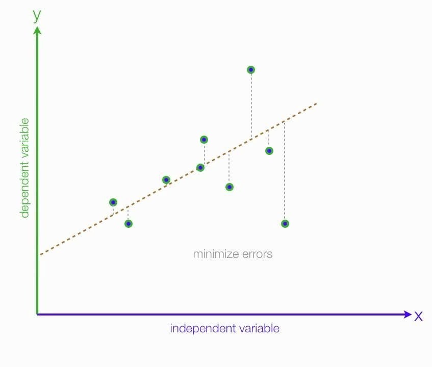
Linear regression is a type of supervised machine learning algorithm that learns from labeled data sets with an input and an output. The machine attempts to create a line that represents a linear relationship between these two numbers, allowing it to predict the output, the dependent variable, based on the input, the independent variable. The line follows the equation

y = wx + b

 where x is a numerical input, w is the weight/slope of the line, b is the bias/y-intercept, and y is the output. To try to predict the output based on the input, the machine multiplies the input by the weight and then adds the bias. The weights are initially random, resulting in inaccurate outputs, but the model adjusts them accordingly to minimize the error. Over time, the line gradually shifts until it most closely aligns with the data.

The actual equation that the LinearRegression model used was:

y = w₁ x₁ + w₂ x₂ + w₃ x₃ + w₄ x₄ + w₅ x₅ + w₆ x₆ + w₇ x₇ + w₈ x₈ + w₉ x₉

• Y = predicted next-day stock price
  
  
• x₁, x₂, …x₉ = the nine input features (3 open prices, 2 close prices, 1 volume,  1 stock dividends, 1 high, and 1 stock split)
  
  
• w₁, w₂, …w₉​ = the learned coefficients (model weights)
  
  
• B = the intercept term (bias)

Linear regression is frequently used as a baseline model in financial time-series forecasting due to its interpretability and robustness in short-horizon settings. Prior studies have shown that linear regression can perform competitively for next-day price prediction, particularly when feature windows are small and market noise dominates the signal. Li, Shengzhou demonstrates that linear models often capture short-term momentum effectively, even when more complex nonlinear structures are present⁶. Similarly, other studies such as Yuqing Zhao’s note that linear regression remains reliable when external contextual data, such as sentiment or macroeconomic indicators, are absent. This study builds upon this literature by confirming that, when limited to a three-day input window, linear regression generalizes better than more complex models, not because markets are linear, but because simpler estimators are less prone to fitting noise⁷.

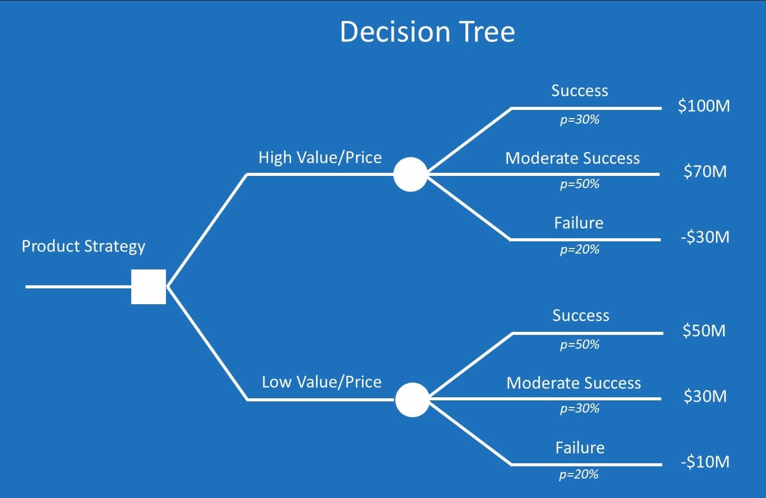
Decision Tree

Next, we create a decision tree model with scikit-learn called DecisionTreeRegressor, train the model on the training data, and then evaluate the model on the training and testing data using mean squared error. A decision tree is a type of supervised learning algorithm that works like a series of nested if statements that determine which branch of the tree to follow next. The first decision starts with a root node, and the outgoing branches feed into the internal nodes, known as decision nodes. The machine builds the tree based on training data to determine how to create questions for each internal node optimally. Decision trees are more accurate the smaller they are, because they can separate the data so each branch contains a large amount of similar data points. However, as a tree grows in size, each branch has a small number of data points, which makes the model too specific for the training data. This causes overfitting, where the tree memorizes the training data instead of learning patterns that can be applied to new data. A way that decision trees can maintain their accuracy by expanding the number of branches is through a random forest algorithm.

The max_depth parameter determines how many levels of decisions the model can make before reaching a final prediction, effectively controlling its complexity. A smaller depth (such as 3) restricts the tree to broader, higher-level splits, which helps the model capture only the most general relationships in the data — for instance, overall upward or downward price movements. This prevents the tree from reacting too strongly to short-term market noise or outliers. In contrast, a larger depth (such as 10) allows the tree to continue splitting the data into increasingly specific groups, enabling it to learn more intricate patterns and conditional relationships between variables. However, excessive depth increases the risk of overfitting, where the model memorizes subtle fluctuations unique to the training period rather than learning generalizable trends. By experimenting with two depths, 3 and 10, we aimed to observe how increased model flexibility affects prediction accuracy and whether added complexity leads to improved generalization or merely captures random variation in stock behavior.

Random Forest

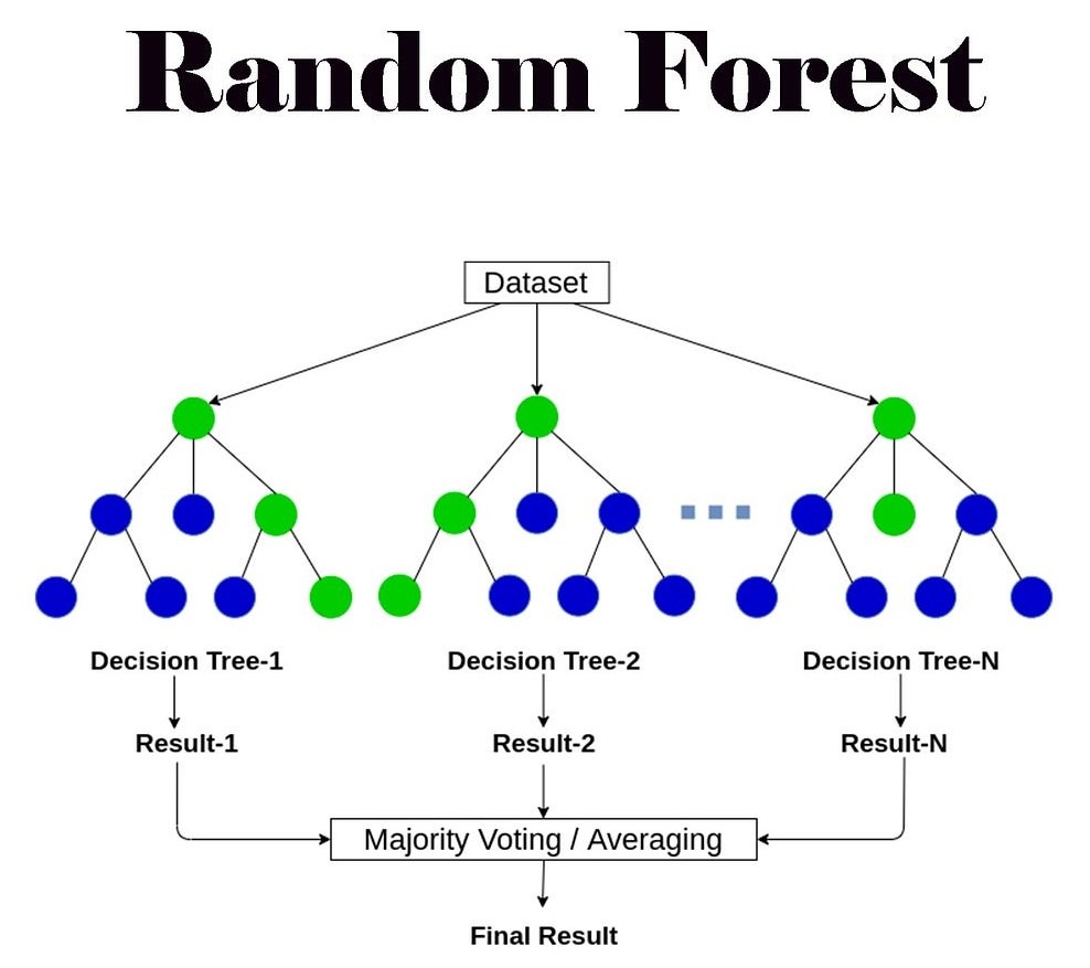
Next, we create a random forest model with scikit-learn called RandomForestRegressor, train the model on the training data, and then evaluate the model on the training and testing data using mean squared error. A random forest is a machine learning model that combines the outputs of multiple decision trees to reach one single output. So instead of relying on one decision tree, the random forest builds a whole forest of trees that are each trained on different pieces of data. The forest makes its final prediction by averaging the predictions for numbers, or counting up output decisions for classification. The parameter n_estimators sets the number of individual trees in the forest, where each tree has a depth determined by the parameter max_depth.

The parameter n_estimators was set to 40 and 60 in our experiments. These values were chosen to balance model stability and computational efficiency. In random forests, a larger number of trees generally reduces variance and improves prediction stability, but the improvement plateaus after a certain point while training time and resource usage continue to increase. Preliminary tests showed that performance gains leveled off beyond approximately 60 trees, with only negligible reductions in mean squared error. Therefore, using 40 and 60 estimators allowed us to evaluate model stability across a moderate and high ensemble size without unnecessary computational cost. This range ensured that the forest was large enough to capture diverse decision boundaries while still maintaining practical efficiency for repeated experiments across multiple stocks.

Tree-based models are widely used in financial prediction due to their ability to model nonlinear relationships and interactions among features. Prior studies by Rady, E. H., et al. have shown that single decision trees often overfit financial data, while ensemble methods such as random forests can reduce variance and improve stability by averaging across multiple trees⁸. Research by Stoll, F on tree-based time-series forecasting consistently finds that random forests outperform individual trees but still require careful tuning and sufficient data to generalize effectively. This study builds on that work by confirming that decision trees achieved strong training performance but failed to generalize, while random forests offered modest improvements yet still underperformed simpler models in short-horizon prediction⁹. These results suggest that although ensemble methods mitigate overfitting, they remain limited when trained on narrow historical windows without external information.

Neural Network

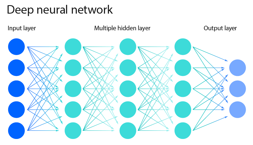
Next, we create a neural network model with scikit-learn called MLPRegressor, train the model on the training data, and then evaluate the model on the training and testing data using mean squared error. A neural network is a type of machine learning model that is supposed to make decisions in a similar way to how human brains do. A neural network is comprised of layers of neurons, known as nodes, that process information. The first layer of the neural network is called the input layer, and this layer takes in raw input in number form. Then, each neuron takes the input number it receives, and this number travels through the “lines”, or parameters of the neural network. Every time a number passes through a line, it is multiplied by a specific weight of the line, which represents the importance of the input. Then, after multiplying, the neuron adds those results together. Once this number is calculated, the neuron runs the number through a specific function that decides whether the number should pass onto the next layer. If the number is negative, then the function makes the number 0. This same process applies to each hidden layer in the neural network, as well as the output layer.

Over time, the machine improves the accuracy of the output by adjusting the weights across each parameter. The weights are initially random, but as the model continues to run, they change to increase or decrease the weight based on the accuracy compared to the correct output. Over time, the network learns which parameters should have the most weights, so it can accurately output the correct number.

The parameter hidden_layer_sizes determines the number of neurons in each hidden layer of the neural network. In our experiments, we tested architectures with 10 and 50 neurons. These values were selected to represent both a lightweight network capable of learning basic linear and nonlinear trends, and a moderately deep network with greater capacity to capture complex temporal relationships in stock movements. Networks with fewer than 10 neurons tended to underfit, failing to model nonlinearity in price changes, while those with more than 50 neurons showed early signs of overfitting—performing well on training data but poorly on testing data.

The parameter max_iter, which defines the maximum number of iterations the algorithm uses to adjust weights during training, was set to 60 and 100 for our experiments. These values were chosen to allow sufficient optimization without causing excessive computation time or convergence issues. Preliminary trials indicated that increasing max_iter beyond 100 did not improve performance meaningfully, as the model reached convergence before completing all iterations. Together, these parameter choices offered a practical tradeoff between training efficiency and generalization ability across multiple stock datasets.

Neural networks and deep learning models dominate recent financial forecasting literature due to their ability to learn complex nonlinear and temporal dependencies. A study from Moghar, A. et al. using LSTMs reported strong performance when models are trained on long historical sequences and enriched with external features such as sentiment, macroeconomic indicators, or technical signals. This research shows that models designed to learn patterns over time can outperform simpler approaches, which helps explain why neural networks are used, but also why they struggle when only limited historical data is available¹⁰. This study differs from much of the deep-learning research, such as Zhang C’s work using CNNs, Transformers, and RNNs, which shows that neural models can capture complex nonlinear patterns, but only when enough data and context are available. If there is not, neural networks exhibit severe overfitting and highly negative testing R² values¹¹.

K-nearest neighbors

Next, we create a K-nearest neighbors model using scikit-learn’s KNeighborsRegressor, train the model on the training data, and then evaluate the model on both the training and testing data using the mean squared error (MSE). The K-nearest neighbors method is a supervised learning model that makes predictions based on the closeness of data points. For classification, the algorithm checks the labels of those k neighbors and assigns the new point the majority label (like a “vote”). For regression, the prediction is usually the average value of the neighbors’ outputs. The choice of the number of neighbors as a parameter determines how many nearby points the model looks at to make its prediction.

K-nearest neighbors has been explored in financial forecasting as an instance-based learning method that predicts prices based on historical patterns most similar to recent observations. However, prior research from Kumbure, M. M. reports that KNN struggles with volatile and nonstationary financial time series, as similarity in price space does not necessarily imply similarity in future movement. Reviews of machine learning models for stock prediction emphasize that KNN is highly sensitive to noise and scaling issues, often leading to poor generalization in out-of-sample testing¹². This study aligns with David Iyanuoluwa Ajiga’s work that discusses ensemble ML methods including KNN alongside other algorithms that, across multiple stocks produced low or negative testing R² values, reinforcing the view that proximity-based methods are ill-suited for short-term financial forecasting without strong feature engineering or volatility normalization¹³.

Calculating Error

In addition to the Mean Squared Error (MSE), we evaluated model performance using the coefficient of determination (R²) to provide a broader assessment of predictive accuracy. R² measures how well the model explains the variance in the actual stock prices, with values closer to 1 indicating a stronger fit. This metric complements MSE by revealing how effectively each model captures the underlying patterns and variability in the data, rather than just minimizing average error magnitude. It is important to note that R² is scale-invariant, which means it allows fair comparison across stocks with different price levels and volatilities.

The next cell creates a combined prediction by averaging the outputs of the five models, each model contributing 20% of the average. We then calculate the mean squared error of this averaged prediction for both the training data and the testing data.

This next cell creates a weighted prediction of the five models based on their accuracy. First, we calculate the inverse of each model’s mean squared error on the test data, so that models with lower MSE, and therefore better accuracy, receive higher scores. These scores are then normalized by dividing each one by the total sum, turning them into weights that add up to 1. Using these weights, we combine the models’ predictions into a weighted average, giving more substantial influence to models that performed better and less to those that performed worse. Finally, we evaluate this weighted prediction against the actual test values using mean squared error. Unlike the simple average, where each model contributed equally, this approach adjusts the contribution of each model according to its accuracy.

Instead of recalculating model weights using realized test errors, we compute a single fixed weight for each model based solely on its performance on the training data. Specifically, each model’s weight is derived from the inverse of its training mean squared error, ensuring that models with lower training error receive greater influence. These weights are then normalized so that they sum to one and are locked before evaluation. During testing, the final prediction for each input is produced by taking a weighted average of the models’ outputs using these fixed weights. This approach avoids any access to future information or test targets and provides a fair assessment of ensemble performance while maintaining consistency with realistic forecasting constraints.

In this next section, we run a simple simulation to test whether our model’s predictions could have generated profit in practice. Starting with $10,000 in cash, the simulation uses the model’s predicted prices to decide when to buy or sell: If the prediction for the next day is higher than today’s price, we buy a share (if we have enough cash), and if the prediction is lower, we sell a share (if we own any). At the end of the period, we sell off any remaining shares and compare the final amount of money to the starting balance. The result shows the simulated profit or loss, giving us a way to evaluate how well the model’s predictions would translate into actual trading performance.

We then expand the simulation to allow for trading multiple shares at once rather than just a single share per transaction. Starting with the same $10,000 in cash, the updated strategy buys two shares whenever the model predicts the next day’s price will be higher and sufficient funds are available. Similarly, it sells two shares whenever the prediction suggests a price drop and at least two shares are currently held. At the end of the simulation period, any remaining shares are sold at the final day’s price, and the total value is compared to the initial $10,000. This approach provides a more realistic trading scenario, since investors typically buy and sell more than one share at a time, and it allows us to see whether scaling up the trades amplifies profits or losses based on the model’s predictions.

Result

To evaluate the effectiveness of each model, we compared its mean squared error (MSE) on both training and testing data across six major companies.

	Apple (AAPL)	JPMorgan Chase (JPM)	Pfizer (PFE)	Tesla (TSLA)	ExxonMobil (XOM)	Walmart (WMT)
linearmodel	2.11 ± 0.00	1.49 ± 0.00	0.013 ± 0.00	24.02 ± 0.00	0.73 ± 0.00	0.12 ± 0.00
Decisiontree (max_depth=3)	10.04  ± 0.00	10.05 ± 0.00	0.80 ± 0.00	107.15 ± 0.00	8.13 ± 0.00	0.53 ± 0.00
Decisiontree (max_depth=10)	0.17 ± 0.00	0.15 ± 0.00	0.00 ± 0.00	1.80 ± 0.00	0.08 ± 0.00	0.01 ± 0.00
randomforest(max_depth=5, n_estimators=60)	1.65  ± 0.01	1.20 ± 0.01	0.09 ± 0.01	18.01 ± 0.16	0.71 ± 0.01	0.09 ± 0.00
randomforest(max_depth=8, n_estimators=40)	0.62 ± 0.01	0.47 ± 0.00	0.03 ± 0.00	7.18 ± 0.05	0.24 ± 0.01	0.03 ± 0.00
Neural network(hidden_layer_sizes=(50,),max_iter=100)	647.57 ± 6158.94	22.66 ± 1745.55	625.75 ± 636.82	18848.20 ± 20607.49	465.61  ±  4496.57	76.17 ± 400.30
Neural network(hidden_layer_sizes=(10,),max_iter=60)	2903.18 ± 477975.76	126.52 ± 8296.4	609.25 ± 691580994.65	1572.73 ±  52230.39	4081.81 ±  860.74	184.41 ±  1444.49
KNeighbors(n_neighbors=5)	275.01 ± 0.00	212.60 ± 0.00	30.77 ± 0.00	2083.76 ± 0.00	345.01 ± 0.00	11.39 ± 0.00
KNeighbors(n_neighbors=10)	306.70 ± 0.00	243.53 ± 0.00	34.07 ± 0.00	2357.50 ± 0.00	388.51 ± 0.00	12.41 ± 0.00

	Apple (AAPL)	JPMorgan Chase (JPM)	Pfizer (PFE)	Tesla (TSLA)	ExxonMobil (XOM)	Walmart (WMT)
linearmodel	7.43 ± 0.00	4.54 ± 0.00	0.03 ± 0.00	44.67 ± 0.00	0.65 ± 0.00	0.49 ± 0.00
Decisiontree (max_depth=3)	1438.16 ± 0.00	6370.00 ± 0.00	18.88± 0.00	1062.56 ± 0.00	80.22 ± 0.00	975.31± 0.00
Decisiontree (max_depth=10)	1091.73 ± 35.49	4852.66 ± 0.00	13.50  ± 0.12	590.10  ± 0.46	21.67 ± 0.75	879.83 ± 0.00
randomforest(max_depth=5, n_estimators=60)	1174.21 ± 1.88	5089.99 ± 24.16	15.13 ± 0.07	505.25 ± 17.43	26.86 ± 0.12	901.08 ± 2.00
randomforest(max_depth=8, n_estimators=40)	1125.37 ± 5.86	4902.48 ± 6.98	14.18 ± 0.09	447.40 ± 17.03	22.48 ± 0.09	892.40 ± 6.70
Neural network(hidden_layer_sizes=(50),max_iter=100)	2702.06 ± 57236.42	142.18 ± 8180.897	776.36± 213.74	26418.27 ± 152928.00	462.43  ±  15882.15	151.70 ± 1071.17
Neural network(hidden_layer_sizes=(10,),max_iter=60)	12683.40 ± 115053.01	923.79 ± 7084.09	819.92 ± 1104.00	1700.82 ± 36.12	9752.97 ± 3754.97	1236.7 ± 15238.01
KNeighbors(n_neighbors=5)	3515.90 ± 0.00	11644.85 ± 0.00	138.16 ± 0.00	11341.14 ± 0.00	883.73 ± 0.00	1559.59 ± 0.00
KNeighbors(n_neighbors=10)	3484.81 ± 0.00	11575.46 ± 0.00	129.50 ± 0.00	10682.25 ± 0.00	891.09 ± 0.00	1563.21 ± 0.00

Model	Apple (AAPL)	JPMorgan Chase (JPM)	Pfizer (PFE)	Tesla (TSLA)	ExxonMobil (XOM)	Walmart (WMT)
Linear Regression	0.9956 ± 0.0000	0.9951 ± 0.0000	0.9968 ± 0.0000	0.9925 ± 0.0000	0.9988 ± 0.0000	0.9920 ± 0.0000
Decision Tree (max_depth = 3)	0.9792 ± 0.0000	0.9672 ± 0.0000	0.9797 ± 0.0000	0.9664 ± 0.0000	0.9861 ± 0.0000	0.9653 ± 0.0000
Random Forest (max_depth = 5, n_estimators =60)	0.9966 ± 0.0000	0.9961 ± 0.0000	0.9976 ± 0.0000	0.9944 ± 0.0000	0.9988 ± 0.0000	0.9942 ± 0.0000
Neural Network (hidden_layer_sizes = (50), max_iter = 100)	−14.07 ± 2.80	−12.02 ± 13.10	−43.16 ± 31.03	−39.32 ± 38.60	−25.19 ± 13.91	−56.35 ± 80.97
K-Nearest Neighbors (n_neighbors = 10)	0.3659 ± 0.0000	0.205 ± 0.000	0.139 ± 0.000	0.261 ± 0.000	0.336 ± 0.000	0.193 ± 0.000

Model	Apple (AAPL)	JPMorgan Chase (JPM)	Pfizer (PFE)	Tesla (TSLA)	ExxonMobil (XOM)	Walmart (WMT)
Linear Regression	0.9954 ± 0.0000	0.9984 ± 0.0000	0.9982 ± 0.0000	0.9949 ± 0.0000	0.9978 ± 0.0000	0.9987 ± 0.0000
Decision Tree (max_depth = 3)	0.1090 ± 0.0000	−1.2868 ± 0.0000	−0.1007 ± 0.0000	0.8783 ± 0.0000	0.7344 ± 0.0000	−1.5881 ± 0.0000
Random Forest (max_depth = 5, n_estimators = 46)	0.2732 ± 0.0010	−0.815 ± 0.003	0.119 ± 0.003	0.944 ± 0.001	0.910 ± 0.000	−1.366 ± 0.007
Neural Network (hidden_layer_sizes = (50), max_iter = 100)	−8.47 ± 10.12	−15.49 ± 25.10	−107.13 ± 134.60	−8.50 ± 4.70	−29.56 ± 16.65	−14.49 ± 21.88
K-Nearest Neighbors (n_neighbors = 10)	−1.1591 ± 0.0000	−3.156 ± 0.000	−6.549 ± 0.000	−0.223 ± 0.000	−1.950 ± 0.000	−3.148 ± 0.000

The table below compares the stock prices of six major companies, showing their type, quantity, and period of data

Company	Ticker	Data Type	Period	Quantity	Original Price	Final  Price
Apple	AAPL	Daily stock price (Yahoo Finance via yfinance)	Sep 2020 – Sep 2025	~1,260	110.84	240.00
JPMorgan Chase	JPM	Daily stock price (Yahoo Finance via yfinance)	Sep 2020 – Sep 2025	~1,260	90.04	303.65
Pfizer	PFE	Daily stock price (Yahoo Finance via yfinance)	Sep 2020 – Sep 2025	~1,260	27.35	24.27
Tesla	TSLA	Daily stock price (Yahoo Finance via yfinance)	Sep 2020 – Sep 2025	~1,260	118.67	348.00
ExxonMobil	XOM	Daily stock price (Yahoo Finance via yfinance)	Sep 2020 – Sep 2025	~1,260	30.79	111.60
Walmart	WMT	Daily stock price (Yahoo Finance via yfinance)	Sep 2020 – Sep 2025	~1,260	43.97	101.08

Stock	Model	Test MSE	Test R²
AAPL	ARIMA (1,0,0)	5561.6754	-2.2562
JPM	ARIMA (1,0,0)	8884.0508	-1.9495
PFE	ARIMA (1,0,0)	30.4091	-0.8316
TSLA	ARIMA (1,0,0)	14001.2176	-0.4878
XOM	ARIMA (1,0,0)	287.6700	0.0457
WMT	ARIMA (1,0,0)	1519.0692	−3.1433

Across all six companies, linear regression achieved the lowest testing MSE values overall, indicating that simple linear relationships captured short-term stock behavior better than more complex nonlinear models. In contrast, decision trees, random forests, neural networks, and K-nearest neighbors (KNN) exhibited much higher testing errors, suggesting overfitting or instability in capturing generalizable patterns. This aligns with the nature of financial data, which is highly stochastic and often dominated by noise rather than clear nonlinear trends. The linear model’s ability to generalize across datasets highlights that short-term market changes can often be approximated by recent historical momentum rather than intricate temporal dependencies. On the other hand, the poor testing performance of deeper trees, random forests, and neural networks reveals that complex models may have captured spurious relationships within training data rather than meaningful predictive signals.

The substantial gap between training and testing MSEs—particularly for neural networks and KNN—indicates significant overfitting. For example, the neural network with hidden_layer_sizes=(50) achieved extremely low training error on some stocks (e.g., Pfizer, 625.75) but drastically higher testing error (e.g., 776.36), demonstrating that the model learned patterns specific to the training data rather than general trends. Similarly, the random forest and deeper decision trees had low training errors but failed to maintain performance on unseen data. This suggests that increasing model complexity without sufficient regularization or cross-validation led to poor generalization. Incorporating a validation step, such as cross-validation or time-based validation, would help ensure model robustness by better balancing training and testing performance. These results reinforce that while more complex models can memorize past behavior, they often fail to extrapolate effectively in dynamic financial environments.

Across all six companies, the R² results reveal consistent patterns in model performance and underscore the challenges of predicting short-term stock prices using limited historical data. Linear regression achieved the highest and most stable R² values—ranging from roughly 0.99 to 0.998—across both training and testing sets. This indicates that simple linear relationships explain most of the short-term price variance, likely because the short, three-day input window fails to capture the nonlinear dependencies that more complex models are designed to detect. Random forests also performed strongly, with high training R² values and moderately strong testing scores, suggesting they can generalize better than single decision trees while still being susceptible to minor overfitting. Decision trees performed well in training but suffered significant drops in testing R², confirming their tendency to overfit small datasets. Neural networks exhibited highly unstable and often negative R² values implying poor generalization and occasional divergence during training due to limited data and the absence of external features like sentiment or macroeconomic indicators that such models rely on to learn nonlinear trends. K-nearest neighbors consistently produced low or negative R² values, showing that proximity-based methods struggle in volatile financial data where small fluctuations are not spatially consistent over time. Overall, these results demonstrate that while simple models like linear regression can approximate short-term behavior with high accuracy, more complex architectures require richer, longer, and more diverse datasets to achieve meaningful predictive value in financial markets.

Table 6 presents the testing performance of the ARIMA(1,0,0) baseline model across all six stocks. Overall, ARIMA performs poorly relative to the machine learning models presented earlier, with negative R² values for five out of six companies. A negative R² indicates that the model predicts worse than simply using the average of the training data, highlighting ARIMA’s limited ability to capture short-term price movements in this setting. While ARIMA achieves a slightly positive R² for ExxonMobil (XOM), its performance remains substantially weaker than linear regression and other supervised learning approaches. These results suggest that univariate time-series models relying solely on past prices struggle to generalize when the prediction horizon is short and market behavior is dominated by noise. In comparison, supervised models that incorporate multiple recent price features provide a more reliable framework for next-day stock price prediction.

These findings are consistent with prior research on financial time series forecasting, which shows that short-horizon stock prices are often dominated by irregular patterms rather than a predictable structure. Multiple studies have found that simple linear or shallow models can outperform deep or highly flexible architectures when prediction windows are short and feature sets are limited, while complex models only show advantages when trained on long historical windows or enriched with external information such as sentiment, macroeconomic indicators, or volatility measures. Together, this literature reinforces the conclusion that model performance in financial forecasting depends less on algorithmic sophistication and more on the informational richness of the input data^{14‘15‘16‘17}.

Conclusion

The experimental results show that among the five models tested, linear regression consistently achieved the lowest mean squared error (MSE) on the test data. It performed especially well on Pfizer and ExxonMobil. The more complex models, such as decision trees, random forests, neural networks, and K-nearest neighbors, captured additional patterns. However, these often overfit, as demonstrated by lower training MSE and higher testing MSE. Given the narrow input window and the lack of external features like sentiment or macroeconomic data, we should interpret these results cautiously. Future work could incorporate more data sources to see if more complex models can outperform linear regression in a broader context.

Beyond the numerical scores, these results offer insight into how machine learning interacts with real financial markets. This study hypothesized that more complex models, such as neural networks, would outperform simpler models by identifying nonlinear relationships in short-term price movements. Instead, the opposite occurred. This outcome reflects a core challenge in quantitative finance: next-day stock prices are extremely difficult to predict using only recent historical data. Real-world price changes are driven by earnings announcements, economic news, geopolitical events, and investor sentiment, none of which are visible to a model trained strictly on past prices. As a result, models that attempt to learn complex patterns from such limited data end up fitting noise rather than meaningful structure. In practice, this would lead to unstable or misleading trading signals. The strong results of linear regression, therefore, do not imply that financial markets behave linearly; instead, they show that when limited information is available, simpler models remain the most reliable compared to complex models with many variables.

The primary limitation of this study is that stock prices cannot be reliably predicted using only the past three days of data. Market movements are influenced by more complex, longer-term patterns and by external factors that this narrow time frame cannot capture. A better approach that would add context rather than just numerical data is financial sentiment analysis, which allows models to process unstructured data from news articles, analyst reports, and social media posts. This method has been shown to capture investor sentiment—whether positive or negative—and to improve predictive performance when combined with historical price data^18‘19. Similarly, incorporating macroeconomic variables or volatility indices could help account for market conditions that influence short-term price reactions. Expanding the input window beyond three days and using dedicated time-series architectures, such as LSTMs or temporal convolutional networks, would further improve the model’s ability to recognize temporal dependencies^20‘21.

Future research could also examine additional data available on Yahoo Finance, such as closing price, trading volume, dividends, stock splits, or trading highs. We could also test our models with more realistic trading simulations, such as strategies involving buying and selling multiple shares or diversifying across different stocks, to better estimate how these models might perform in practice. For example, sudden policy changes, such as the U.S. tariffs under the Trump administration, produced sharp, sentiment-driven market swings that models based solely on past prices could not predict. Additionally, the trading simulations used in this study do not incorporate crucial real-world constraints such as transaction costs, slippage, liquidity limits, or bid-ask spreads. These limitations reduce the realism and practical applicability of the results, as they can significantly alter trading performance in real markets²².

In the future, we want to add a stock recommendation system. Unlike pure prediction models, a recommendation system suggests specific stocks to users. Its effectiveness depends less on whether the stock price actually rises and more on user behavior, like how easily users click on a recommendation. In this context, success is measured by metrics like click-through rate, which indicates how many people clicked on the suggested stock after seeing it, rather than long-term performance. If the system only recommends the most popular stock every time, it risks overfitting to historical behavior, just like a model can overfit to training data. A better recommendation system would personalize suggestions by asking targeted questions and then evaluate its performance using test data. While metrics like mean squared error can help in development, the accurate measure of success is how well the system performs on unseen data, as shown in testing scores.

Additionally, this study used multiple input features, Open, Close, High, Volume, Dividends, and Stock Splits, but did not explicitly quantify their contribution to model predictions. A feature importance analysis, particularly for tree-based models like the decision tree and random forest, could reveal which variables most strongly influence price forecasting. For example, in similar studies, previous closing prices and trading volume are often found to be the most predictive, as they directly reflect investor sentiment and liquidity trends. Generating a feature importance chart using the .feature_importances_ attribute from scikit-learn’s tree-based models would enhance interpretability and transparency. This would allow readers to understand whether the models rely more on price-based indicators (momentum) or on external variables (volume or dividends), thereby clarifying which financial metrics contribute most to short-term stock movements. Such an addition would make the results more explainable and aligned with best practices in financial machine learning research^23‘24‘25.

Overall, the findings show that when the input data is extremely limited, simple models such as linear regression may outperform more sophisticated algorithms because they avoid overfitting unpredictable short-term fluctuations. The study demonstrates that model complexity alone does not guarantee better predictive performance. What truly matters is the relevance of the input features. To advance short-term stock prediction, future research must focus on expanding the information given to machine learning models, not just increasing algorithmic complexity. Incorporating sentiment data, macroeconomic indicators, longer historical windows, and more realistic simulation frameworks will provide a stronger foundation for assessing whether advanced models can meaningfully improve short-term forecasts in real financial environments.

References

1. T. Phuoc, P. Thi Kim Anh, P. Huy Tam, C.V. Nguyen. Assessing AI-driven stock prediction research. Humanities and Social Sciences Communications Vol. 11, Article number: 393 (2024). [↩]
2. S. Yue Xu. Stock price forecasting using information from Yahoo Finance and Google Trends. University of California, Berkeley (2012). [↩]
3. Jahan, Israt. Stock price prediction using recurrent neural networks. North Dakota State University Library (2018). [↩]
4. A. Chatterjee, H. Bhowmick, J. Sen. Stock price prediction using time series, econometric, machine learning, and deep learning models. Praxis Business School (2018). [↩]
5. P. Tupe-Waghmare. Prediction of stocks and stock price using artificial intelligence: a bibliometric study using Scopus database. Symbiosis Institute of Technology (2021). [↩]
6. Li, Shengzhou. Stock price prediction based on linear regression and significance analysis.” In Proceedings of the 2nd International Conference on Data Science and Engineering (ICDSE), 2025, pp. 596-603 (2025). [↩]
7. Y. Zhao. Stock price prediction based on linear regression. Proceedings of the 4th International Conference on Computing Innovation and Applied Physics (2025). [↩]
8. EL. Houssainy A. Rady, H. Fawzy, A. Mohamed Abdel Fattah. Time series forecasting using tree-based methods.” Journal of Statistics and Applications (2021). [↩]
9. F. Stoll. A comparison of machine learning and traditional demand forecasting models. Clemson University (2020). [↩]
10. A. Moghar, M. Hamiche. Stock market prediction using LSTM recurrent neural network.” Expert Systems with Applications (2020). [↩]
11. C. Zhang, N. Nur Amir Sjarif, R. Ibrahim. Deep learning models for price forecasting of financial time séries. Universiti Teknologi Malaysia (2022). [↩]
12. D. Iyanuoluwa Ajiga, R. Adura Adeleye, T. Sunday Tubokirifuruar, B. Gloria Bello, N. Leonard Ndubuisi, O. Franca Asuzu, O. Rita Owolabi. Machine learning for stock market forecasting: a review of models and accuracy. Finance & Accounting Research Journal. (2024). [↩]
13. M. Mailagaha Kumbure, C. Lohrmann, P. Luukka, J. Porras. Machine learning techniques and data for stock market prediction.” Expert Systems with Applications Vol. 197 (2022). [↩]
14. C. Cappello, A. Congedi, S. De Iaco, L. Mariella. Traditional prediction techniques and machine learning for financial time series. Mathematics 13 (2025). [↩]
15. S. Giantsidi, C. Tarantola. Deep learning for financial forecasting: A review of recent advances. International Review of Economics & Finance (2025). [↩]
16. P. H. Vuong, L. H. Phu, T. H. V. Nguyen, N. D. Le, T. B. Pham, and D. T. Trinh. A bibliometric literature review of stock price forecasting methods. Science Progress Vol. 107 (2024). [↩]
17. S.Gupta, S. Nachappa, N. Paramanandham. Stock market time series forecasting using comparative machine learning methods. Procedia Computer Science (2025). [↩]
18. P. C. Tetlock. Giving content to investor sentiment: The role of media in the stock market. The Journal of Finance Vol. 62 (2005). [↩]
19. T. Loughran, B. McDonald. When is a liability not a liability? Textual analysis, dictionaries, and 10-Ks. The Journal of Finance Vol. 66 (2011). [↩]
20. A. H. Huang, H. Wang, Y. Yang. FinBERT: A large language model for extracting information from financial text. Contemporary Accounting Research Vol. 40 (2023). [↩]
21. K. Du, F. Xing, R. Mao, E. Cambria. Financial Sentiment Analysis: techniques and applications. ACM Computing Surveys. Vol. 56 Issue 9(2024). [↩]
22. A. K. Nassirtoussi, S. Aghabozorgi, T. Y. Wah, D. Ngo. Text mining for market prediction: A systematic review. Expert Systems with Applications Vol 41 (2014). [↩]
23. R. Cervello. Forecasting stock market trend: a comparison of machine learning algorithms. Finance Markets and Valuation (2020). [↩]
24. A.Jafari, S.Haratizadeh. Graph-based prediction of stock price movement using graph convolutional network. Engineering Applications of Artificial Intelligence (2022). [↩]
25. S. Makridakis, E. Spiliotis, V. Assimakopoulos. Statistical and machine learning forecasting methods: concerns and ways forward. PLOS ONE Vol.13 (2018). [↩]