Investigating and Comparing YOLO Models for Roadside Object Detection

Abstract

The problem of roadside object detection is essential for ensuring vehicle safety and preventing life-altering car accidents. A potential solution to this problem is the utilization of deep learning-based object detection models, such as YOLO, that can detect and classify objects. In this paper, we investigate the performance of six different YOLO models for roadside object detection: YOLOv7, YOLOv8, YOLOv9, YOLOv10, YOLOv11, and YOLOv12. We analyzed the performance of these models for detecting and labeling common objects found on roads. Furthermore, we investigated the augmentation techniques mixup and cutmix for improving the performance of these models. Our investigation revealed that YOLOv9 is the best model, as it achieved a precision of 84.8%, a recall of 84.8%, and an F1 score of 84.8% on the KITTI dataset. Our experimentation with different augmentation schemes demonstrated that implementing a mixup with a mixing coefficient of 0.9 further improves the model’s precision by 4.1% and its recall by 1.9%, resulting in an F1 score increase of 3.0%. Similarly, implementing a cutmix at 0.1 increases the model’s precision by 5.3% and its recall by 0.7%, resulting in a F1 score increase of 2.9%. Overall, this work provides several recommendations for training object detection models for roadside object detection.

Keywords: Object Detection, Object Classification, YOLO, Bounding box, Augmentation Schemes, mixup, cutmix

Introduction

As more vehicles and drivers have gotten on the road, there has been a sharp increase in the number of fatal road accidents in the past few years. According to the World Health Organization, over 1.2 million people are killed due to car accidents, and around 20 million others suffer life-altering injuries¹. The consequences of these accidents go beyond the immediate fatalities because they place a strain on healthcare systems and emergency services. As the number of traffic accidents continues to grow, it becomes crucial to identify their main causes and improve the methods of preventing them. In a study done by the U.S. Department of Transportation, it was found that over 94% of vehicle accidents are caused by human error, including factors like distraction, impaired driving, and decision-making mistakes².

One of the most effective ways to address this issue is to introduce additional guidance via the implementation of autonomous safety systems on vehicles. To apply these safety features, one must solve the problem of road object detection and identification. Object detection and identification algorithms on vehicles can warn drivers of oncoming traffic or the possibility of a pedestrian or cyclist crossing in their path. These features can also prevent drivers from getting too close to another car and help them keep track of the road in unlit locations.

Many computer vision algorithms have been developed for this purpose. Template matching is a basic approach to object detection, where a template is used to describe an object, and then objects in captured images are compared to the template to check if they match. Feature extraction and logistic regression classification algorithms are another approach to object detection and classification. A feature detector describes an object’s unique features, like edges and textures³. A trained classifier is then used to classify the object. While these methods are effective in most object detection applications, they often struggle when completing more complex tasks.

One method that has recently shown excellent results in computer vision applications, including object detection and classification, is Convolutional Neural Networks (CNN). CNN’s ability to handle complex and non-linear patterns makes it a prime candidate for being used in autonomous safety mechanisms⁴.

An effective application of CNNs in object detection is the development of the ‘You Only Look Once’ (YOLO) algorithm. In this paper, we examined the performance of different variants of YOLO methods on the popular KITTI (Karlsruhe Institute of Technology and Toyota Technological Institute) dataset⁵ comprising different roadside objects. The dataset contains a collection of images of real-world road scenarios and LIDAR(Light Detection and Ranging) data, along with nine different labels for the images. The different YOLO models used are YOLO v7, v8, v9, v10, v11, and v12. We have done comprehensive testing and tweaking of the models to maximize their effectiveness. A significant way of improving these models is by utilizing data augmentation. Hence, this work aims to compare how different YOLO models perform for object identification and classification tasks, and simultaneously determine the effect of mixup and cutmix-based augmentation schemes on each model.

The rest of this paper is organized as follows: first, related work relevant to this study is analyzed. Next, the dataset and methodologies used are described. This is followed by a detailed discussion of the experiments and results. Finally, the paper concludes with a summary and key findings.

Related Work

Research has been completed in this field already. Yang et al.⁶ present a comprehensive survey of image data augmentation techniques for deep learning, offering a structured taxonomy that includes geometric transformations, photometric adjustments, kernel filtering, and mixing-based methods such as mixup and cutmix. Their work synthesises empirical findings across multiple computer vision tasks, including object detection, demonstrating how augmentation improves dataset diversity and model generalisation. While the study does not propose new augmentation algorithms, it provides an essential conceptual and empirical foundation for understanding the practical role of augmentation in mitigating overfitting and improving detection robustness. This review informs the present work’s selection of mixup and cutmix as augmentation strategies for YOLO-based roadside object detection on the KITTI dataset.

Chen et al.⁷ propose a robust object detection framework for autonomous driving that integrates contrastive learning with semi-supervised co-training and reinforcement learning-driven bounding box augmentation. Published in Security and Safety, their method leverages unlabeled data to enhance robustness against environmental perturbations such as Gaussian noise, rain, and fog. Their focus lies primarily on improving detection stability under adversarial and adverse weather conditions through semi-supervised learning strategies. In contrast, the present study adopts a fully supervised training paradigm and concentrates on evaluating the impact of systematic image-level augmentation (mixup and cutmix) on YOLO model performance, allowing for a controlled analysis of augmentation effects independent of semi-supervised learning dynamics.

Recent reviews of deep learning in autonomous driving systems highlight the central role of convolutional neural networks in real-time perception tasks, including object detection and decision-making⁸. These studies emphasise the importance of accurate and timely detection for Advanced Driver Assistance Systems, particularly in complex roadside environments. This broader context underscores the relevance of optimising detection architectures and training strategies to improve system reliability in safety-critical scenarios. The present work aligns with these objectives by focusing on empirical optimisation of YOLO-based detection performance through augmentation techniques tailored to roadside object detection.

Zhao et al.⁹ introduce RT-DETR, a real-time transformer-based detector that eliminates Non-Maximum Suppression through a hybrid encoder architecture. RT-DETR demonstrates competitive accuracy relative to leading YOLO models while achieving increased inference speed compared to prior transformer-based methods. Although transformer detectors represent a promising alternative to traditional CNN-based architectures, the present study maintains a focused scope by evaluating only YOLO variants. This decision enables a more rigorous and controlled comparison within a single architectural family, providing depth in performance analysis rather than broad cross-paradigm comparison.

Vu et al.¹⁰ address the limitations of standard mixup in object detection through their lossmix framework, which interpolates loss values rather than ground truth labels to better accommodate the structured nature of detection tasks. Achieving state-of-the-art performance on PASCAL VOC and MS COCO, their work highlights the challenges of directly applying classification-oriented augmentation techniques to detection problems. While lossmix proposes an alternative formulation, the present study investigates conventional mixup and cutmix to systematically evaluate how standard augmentation strategies influence YOLO detector performance across different augmentation strengths in autonomous driving contexts.

Zhao et al.¹¹ propose X-Paste, an extension of copy-paste augmentation that employs text-to-image generation guided by CLIP to synthesise diverse training instances without manual annotation. This approach specifically targets data scarcity and class imbalance, improving detection performance for underrepresented categories. While X-Paste focuses on generating novel synthetic data, the present work explores how manipulating existing images through mixup and cutmix influences detection robustness, particularly for roadside-relevant classes such as cyclists and pedestrians.

Jia et al.¹² introduce an enhanced YOLOv5 architecture for autonomous driving applications, integrating structural re-parameterisation, neural architecture search, and improved small object detection layers. Their model reports strong performance on KITTI, achieving high detection accuracy alongside real-time inference speeds. This work exemplifies how architectural refinement can significantly enhance detection effectiveness. In contrast, the present study explores performance gains achievable through training-time augmentation alone, allowing for comparison between architecture-driven and augmentation-driven performance improvements.

Similarly, Zhang et al.¹³ present MobileYOLO, a lightweight YOLOv4 variant designed for deployment on resource-constrained platforms. By reducing parameter count while maintaining competitive accuracy on KITTI, MobileYOLO highlights the trade-offs between efficiency and accuracy in real-world systems. The current study complements this line of research by examining whether augmentation strategies can further enhance detection accuracy without increasing computational overhead.

Wei et al.¹⁴ provide a comprehensive review of the YOLO family within autonomous driving contexts, tracing the algorithm’s progression from early versions to the most recent iterations and summarising architectural improvements and deployment considerations. Their survey situates contemporary YOLO variants within a broader historical and technical framework. Building on this context, the present work conducts an empirical comparison of recent YOLO variants under uniform training conditions, with a particular focus on the influence of mixup and cutmix augmentation on roadside object detection performance using the KITTI benchmark.

Despite extensive research on architectural optimisation and emerging detection paradigms, limited work has systematically examined the interaction between augmentation strength and performance consistency across multiple YOLO variants in autonomous driving contexts. Existing studies tend to isolate either architectural innovation or augmentation technique evaluation, but rarely explore their combined influence under controlled experimental conditions. This study addresses this gap by conducting structured experiments on recent YOLO models, varying mixup and cutmix coefficients to quantify their effects on detection accuracy and robustness. The findings provide practical guidance for selecting augmentation strategies and parameter configurations in safety-critical roadside detection systems, where both precision and resilience to occlusion and environmental variation are essential.

Materials and Methods

Dataset and Pre-processing

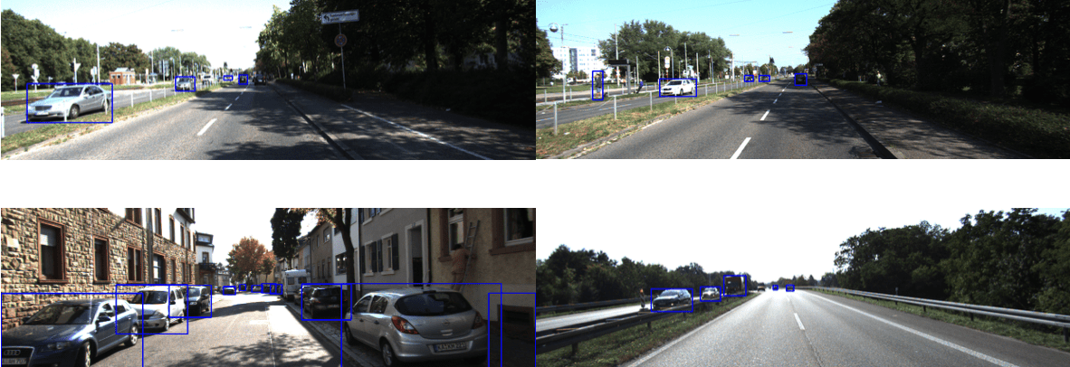
The systematic experiments run for this paper all utilize the KITTI dataset created by Andreas Geiger. The KITTI dataset was recorded from a moving car driving around the streets of Karlsruhe, Germany. The KITTI dataset was selected in this study because it provides a solid foundation for object detection models that need to function in real-world driving environments. The dataset contains images of real traffic situations one may encounter on a road, along with a mix of urban streets, highways, and residential areas. The images in the dataset have consistent image sizes and well-labeled annotations. All of these factors contribute to the KITTI dataset being the ideal dataset for testing the applicability and reliability of a model for roadside object detection. Sample images from the dataset are provided in Fig. 1.

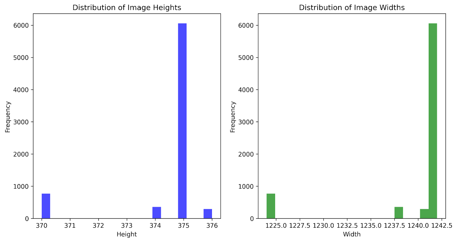
The dataset contains 7,481 images which were taken on daily sidewalks, streets, and roads. Image heights range from 370 to 376 pixels, with an average of 374.5 pixels per image. Image widths range from 1224 to 1242 pixels, with an average of 1239.9 pixels per image. The distributions of image heights and widths are depicted in Fig. 2.

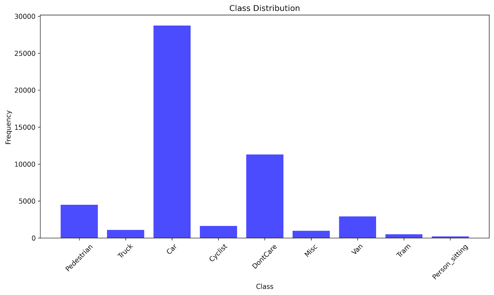
There are 9 different classes of objects in the KITTI dataset, which are divided into these 9 labels: Pedestrian, Truck, Car, Cyclist, DontCare, Misc, Van, Person_sitting, and Tram. In total, there are 51,865 instances of objects. The distribution of classes is as follows: Car (28,742), DontCare (11,295), Pedestrian (4,487), Van (2,914), Cyclist (1,627), Truck (1,095), Misc (973), Tram (511), and Person_sitting (222). A visualization of the class distribution is provided in Fig. 3. The dataset contains more instances of cars than of any other class because cars are the most commonly found objects on roads. Other classes, like Tram or Person_sitting, have fewer instances because they are less frequently found when driving. The mean instances per class is about 5,763, while the standard deviation of instances per class is about 8,747.

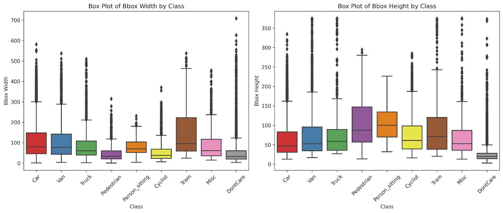
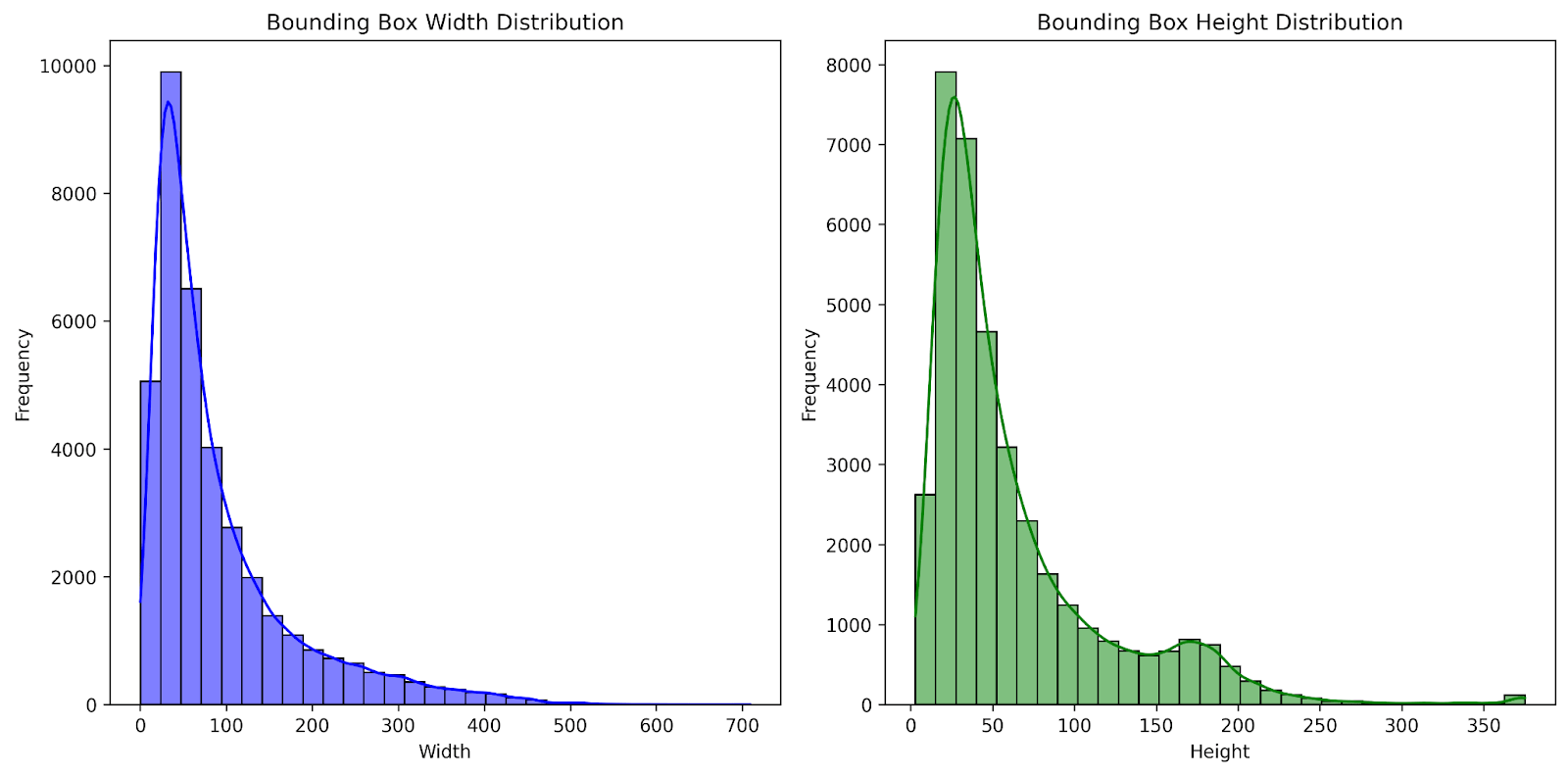
Each instance has a bounding box drawn around it. The majority of the bounding boxes have widths running from 25 to 150 pixels, with an average width of 91.1 pixelsand a median width of 59.7 pixels. The heights of the bounding boxes primarily range from 10 to 75 pixels, with an average height of 63.0 pixels and a median height of 42.5 pixels. Fig. 4 provides a visualisation of the bounding box size distribution for the dataset. The bounding boxes are primarily small because most objects in the images are being captured from a large distance. Fig. 5 displays box plots for bounding box sizes by class. Trams have the largest median width, while pedestrians have the lowest. Pedestrians, however, have the highest median image height, while cars have the lowest.

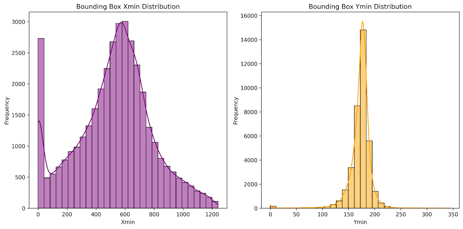
A bounding box’s xmin represents the distance from its leftmost point to the left edge of the image, and its ymin represents the distance from its bottom-most point to the bottom edge of the image.

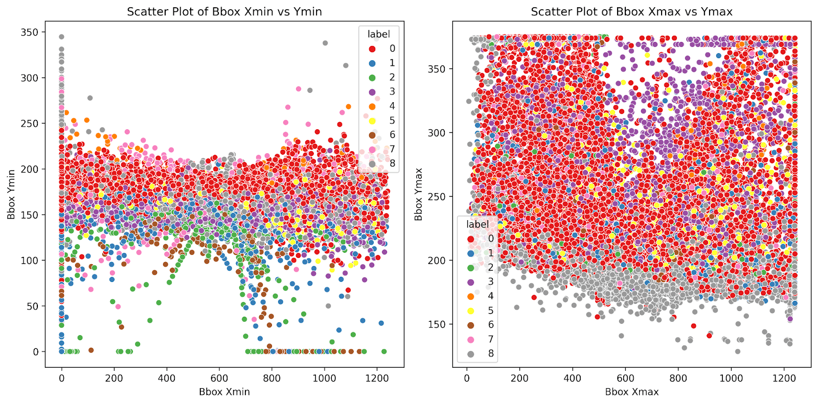
Most of the bounding boxes’ xmin are concentrated between 0 to 40 pixels or 500 to 600 pixels. This suggests the majority of the objects appear on the left side, representing oncoming traffic, or on the center-right side of the image, representing roadside objects. The bounding boxes’ ymin are concentrated between 150 to 200 pixels. This suggests that objects are likely located in the center of the image, where the roadline is located. Fig. 6 shows visualizations of the xmin and ymin distributions for the bounding boxes in the dataset, and Fig. 7 displays a scatter plot for bounding box positions.

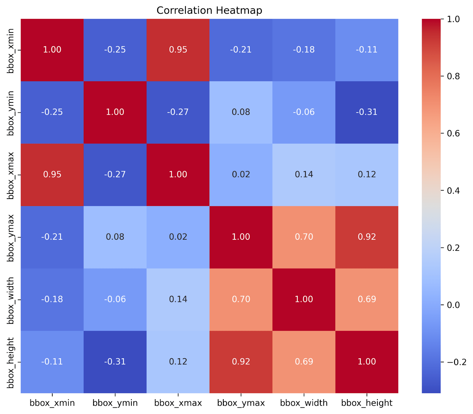
Fig. 8 shows a correlation heatmap between the bounding boxes’ width, height, xmin, ymin, xmax, and ymax values. The relationship between xmin and ymin and the relationship between xmax and ymax each have a strong negative correlation of -0.25 and -0.27, respectively. This suggests that objects on the sides of the image appear to be higher up in the image, while objects in the center of the image appear lower in the image. This pattern reflects how distant or elevated objects appear towards the edges and higher up.

YOLO Models

YOLO (You Only Look Once)¹⁵, proposed in 2015, is a state-of-the-art object detection algorithm that uses an end-to-end neural network to predict bounding boxes and class probabilities simultaneously. Instead of detecting possible regions of interest, YOLO performs all its predictions with connected layers, making it faster than other algorithms like R-CNN(Region-based Convolutional Neural Network), which identifies potential object regions in an image and then uses a neural network to classify what each region contains, or DPM(Deformable Part Models), which represent objects as collections of parts that can flex and move relative to each other while maintaining spatial relationships¹⁶.

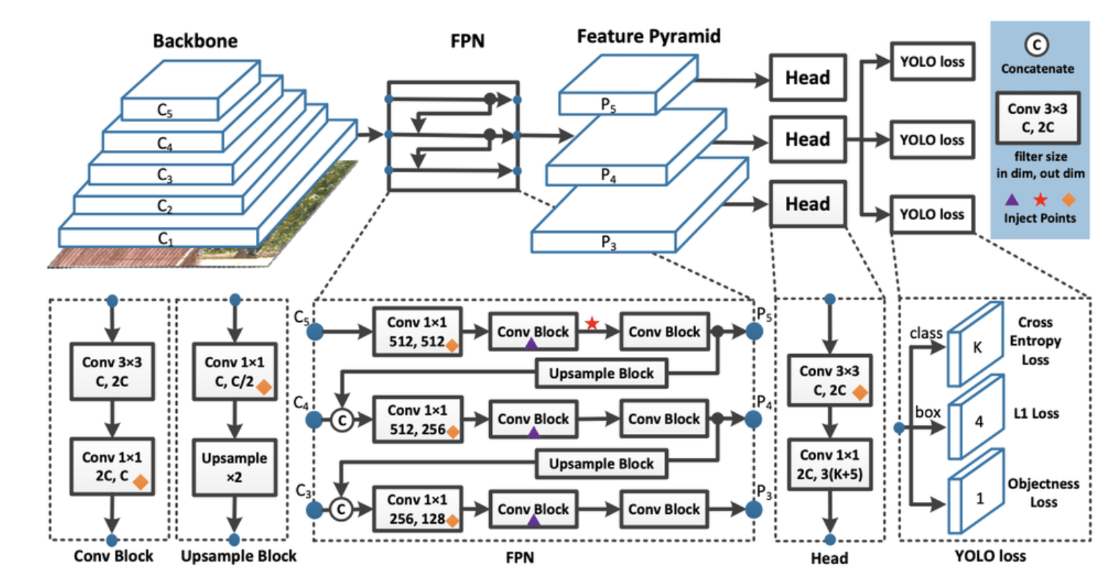
YOLO takes images as inputs and uses a deep convolutional neural network to detect objects in the images. The architecture of the CNN model YOLO utilizes is shown in Fig. 9. YOLO divides the input image into a square grid. When an object is present in the image, each grid cell predicts a bounding box and produces a confidence score for the bounding boxes. Each grid cell can predict multiple bounding boxes, but during training, the algorithm chooses whichever bounding box overlaps most with the actual object location. As training progresses, the grid cells become better at predicting bounding boxes¹⁷.

In this paper, we have implemented YOLO models v7, v8, v9, v10, v11, and v12. Descriptions for each YOLO model implemented are provided below:

YOLOv7

YOLOv7¹⁸, released in July 2022, is a single-stage real-time object detection system. YOLOv7 focuses on the optimization of the training process and introduces several key features and improvements over previous YOLO versions.

It proposes a planned re-parameterized model, a technique that can be used in different types of neural network layers with the concept of gradient propagation path.

The model also introduces a new label assignment method called coarse-to-fine lead guided label assignment. This method starts with a rough decision about which network layer should detect each object, then gradually refines those assignments based on which layers performed the best. The model also proposes extended and compounded scaling methods for the real-time object detector¹⁹.

Compared to previous models, YOLOv7 reduces parameter count by 40% and computation by 50%, while achieving a faster inference speed and a higher detection accuracy.

YOLOv8²⁰, released by Ultralytics in January 2023, builds on the advancements of previous yolo versions and introduces new features and optimizations. The model employs backbone and neck architectures. The backbone extracts features from raw images, and the neck combines and organizes these features. This allows the head to make final predictions on the object locations and classifications. This results in improved feature extraction and object detection performances.

YOLOv8 also adopts an anchor-free split Ultralytics head. This directly predicts object locations without using predefined anchor boxes, which results in better accuracy and a more efficient detection process. YOLOv8 offers a range of pre-trained models specific to various tasks and performance requirements, making it applicable to multiple use cases.

YOLOv8 focuses on maintaining an optimal balance between accuracy and speed. Performance-wise, YOLOv8 achieves faster inference speed than most other object detection models while maintaining a high level of accuracy.

YOLOv9

YOLOv9²¹, released in February 2024, introduces innovative approaches to overcoming the information loss challenge inherent in neural networks. The model improves learning capacity and ensures retention of crucial information through implementing programmable gradient information (PGI) and a generalized efficient layer aggregation network (GELAN).

PGI is implemented to address the information bottleneck problem. The information bottleneck principle reveals that as data passes through successive layers of a network, the potential for information loss increases. The technique uses an auxiliary reversible branch to allow for the generation of reliable gradients. This results in more accurate model updates, improving overall detection performance.

The implementation of GELAN allows YOLOv9 to improve its parameter utilization and computational efficiency. GELAN is a lightweight architecture that combines features from different network layers. This helps make YOLOv9 adaptable to a wide range of applications without sacrificing its speed or accuracy.

YOLOv10

YOLOv10²², released in May 2024 by researchers at Tsinghua University, addresses post-processing and model architecture deficiencies present in previous YOLO versions. YOLOv10 eliminates non-maximum suppression(NMS) and optimizes various model components to reduce computational overhead and improve performance.

The architecture of YOLOv10 is similar to the architecture of previous YOLO versions, but it introduces several new features. The model’s architecture consists of a backbone and neck similar to those of previous models; however, it features two heads. YOLOv10 utilizes a one-to-many head that generates multiple predictions per object during training, and a one-to-one head that generates the single best prediction per object during inference.

The one-to-one head utilized during inference removes the need for NMS. YOLOv10 also incorporates a holistic efficiency-accuracy-driven model design. Efficiency enhancements include lightweight classification heads using depth-wise separable convolutions, spatial-channel decoupled downsampling that separates spatial and channel processing to reduce information loss, and rank-guided block design that adapts architecture based on redundancy to optimize parameter utilization. All of these techniques minimize inference latency and computational overhead while maintaining accuracy.

YOLOv11

YOLOv11²³, released in September 2024 by Ultralytics, contains improvements in architecture and training methods over previous YOLO models. YOLOv11 has many model variants, each applicable to specific tasks like pose estimation, instance segmentation, image classification, object detection, or oriented object detection.

YOLOv11 employs an enhanced backbone and neck architecture, which enhances the feature extraction capabilities of the model. YOLOv11 is optimized for efficiency and speed. YOLOv11 can also be deployed across various environments. This includes edge devices, cloud platforms, and systems supporting NVIDIA GPUs

YOLOv11 has been able to achieve higher accuracies than some previous YOLO models with fewer parameters. When implemented on the COCO dataset, YOLOv11 achieved a higher accuracy than YOLOv8 with 22% fewer parameters.

YOLOv12

YOLOv12²⁴, released in 2025, was developed by researchers from the University of Buffalo, SUNY, and the University of Chinese Academy of Sciences. It introduces an attention-centric architecture different from the traditional CNN-based approaches used in previous YOLO models.
The attention-centric architecture YOLOv12 employs focuses on an image’s important areas, rather than treating every part of the image equally. This cuts down on unnecessary processing, making the model sharper and more efficient. YOLOv12 also utilizes FlashAttention, a memory-efficient algorithm, to speed up image analysis. FlashAttention optimizes data strain and uses less memory.

YOLOv12 organizes its layers using Residual Efficient Layer Aggregation Networks (R-ELAN). R-ELAN is a feature aggregation model based on ELAN, designed to address optimization challenges. It incorporates block-level residual connections and a bottleneck-like structure. R-ELAN makes training more stable and object recognition sharper.

YOLOv12 comes in different variants optimized for different applications. Smaller versions prioritize speed, while medium and large versions strike a balance between speed and accuracy. Because of its architecture, YOLOv12 is expected to run slower than previous YOLO models like YOLOv11.

Experiments and Results

Training and Implementation Details

All models were implemented using their small variant and initialized with pretrained weights from the COCO (Common Objects in Context) dataset. The dataset was split into 72% for training, 8% for validation, and 20% for testing using random sampling with a fixed seed of 42. Training was conducted for 100 epochs with a batch size of 16 and input image dimensions of pixels, using the NVIDIA Tesla P100 GPU. The model was trained using a Stochastic Gradient Descent optimizer configured with an initial learning rate of 0.01, momentum of 0.937, and weight decay of 0.0005. The learning rate schedule employed linear decay with a final learning rate fraction of 0.01, resulting in a final learning rate of 0.0001 by the end of training, along with a 3-epoch warmup period starting from a warmup momentum of 0.8. Data augmentation techniques included mosaic augmentation, color space adjustments (hue=0.015, saturation=0.7, value=0.4), horizontal flipping with 50% probability, random translation of 10%, and scaling with a gain of 0.5. Non-Maximum Suppression used an IoU threshold of 0.7 and a confidence threshold of 0.001 for validation. Each model employs a composite loss function consisting of three weighted components: bounding box regression loss with a gain of 7.5, classification loss with a gain of 0.5, and Distribution Focal Loss with a gain of 1.5 for refined box localization. The architectures use Sigmoid Linear Unit activation functions throughout the network. All experiments used the Ultralytics library, and were conducted on Kaggle, a popular platform for machine learning projects.

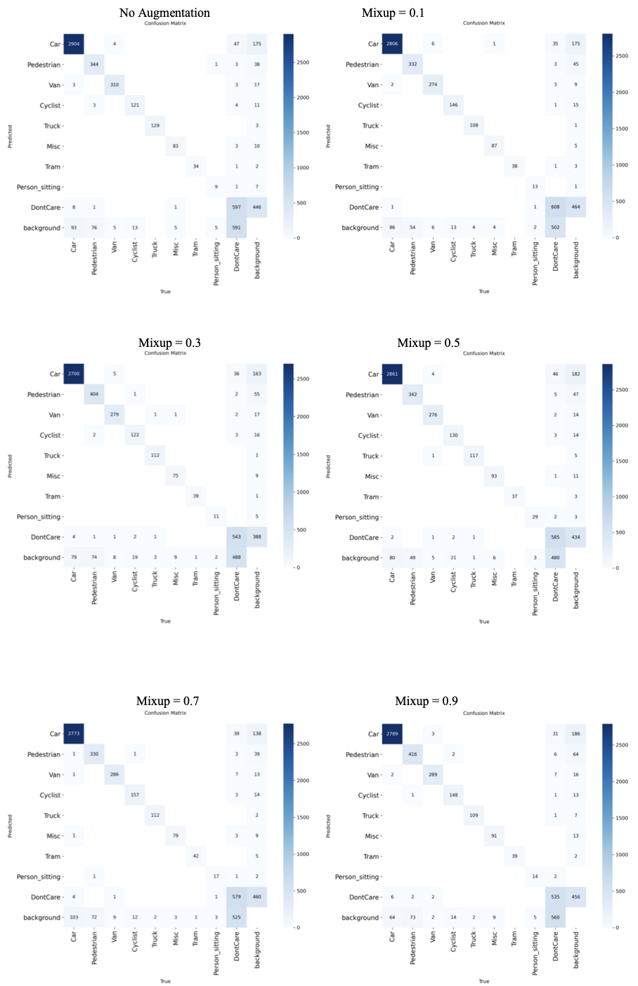
Two additional augmentation schemes have been implemented on YOLOv9: mixup and cutmix. Mixup blends two images and their labels to help the model identify objects when they are partially obscured or blurred. The mixup coefficient controls the probability of applying the augmentation. For YOLOv9, it has been kept as 0.1, 0.3, 0.5, 0.7, and 0.9. On the other hand, cutmix takes a rectangular region out of one training image and pastes it onto another image. This creates realistic occlusion examples for the model to train on, improving the robustness of the model. The cut mix hyperparameter controls the probability of adding the augmentation to a given training image. For YOLOv9, the cutmix coefficient has also been kept as 0.1, 0.3, 0.5, 0.7, and 0.9.

Performance Metrics

The performance metrics we have used in our research are precision, recall, Mean Average Precision(mAP), and F1 score. A confusion matrix has been made for each experiment run, and mAP has been measured at a 50% overlap threshold and a 50% to 90% overlap threshold.

Precision measures the percent of correct predictions out of all predictions made in the positive class. The formula for precision is shown in the equation below. TP denotes true positive(a real object that the detector correctly found), while FP denotes false positive (detected an object that wasn’t actually there).

(1)  

Recall measures the percentage of objects the model detected out of the total number of objects in the dataset. The formula for recall is shown in the equation below. FN denotes false negatives(a real object that the detector missed).

(2)  

The Mean Average Precision(mAP) measures how well a model performs across the entire confidence spectrum. It is calculated by taking the area under the curve formed by a precision vs recall graph. Averaging out the area under this curve for all classes will provide the mAP.

The last metric used is F1 score. F1 score calculates the harmonic mean of precision and recall. It provides a balanced score between the precision and recall. The formula for F1 score is shown in the equation below.

(3)  

All of these relationships can be viewed using a confusion matrix.

Performance of different YOLO models

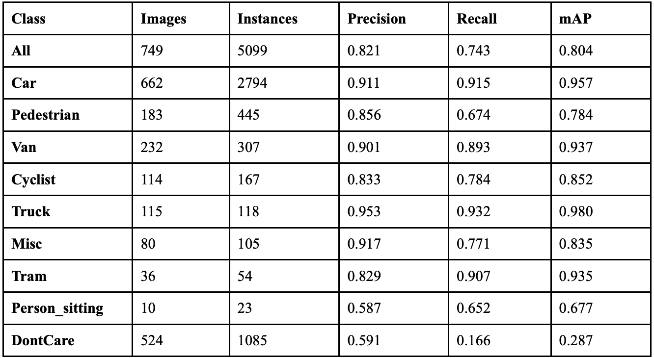
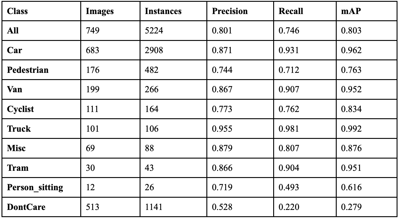
Our experiments showed that YOLOv7 achieved an overall precision of 82.1%, a recall of 74.3%, a mAP50 of 80.4%, and a mAP50-95 of 57.4%. It took 3.062 hours to train for 100 epochs, and resulted in an F1 score of 0.780. Table 1 further shows the class-wise performance of YOLOv7. The model’s detection pipeline often fails between the detection and classification stages. 837 of the real objects the model detected were classified as background during the final prediction, but the model wrongly predicted 387 objects. This suggests the model’s NMS is simultaneously under-suppressing false positives and over-suppressing valid detections. This is likely because of bounding box regression errors and an inconsistent application of IoU(Intersection over Union) thresholds, which is the measure of how much predicted boxes overlap with each other to decide which duplicates to remove. The bounding boxes that YOLOv7 draws are slightly misaligned, so when the NMS tries to remove duplicates, it accidentally deletes the real object while keeping the fake one.

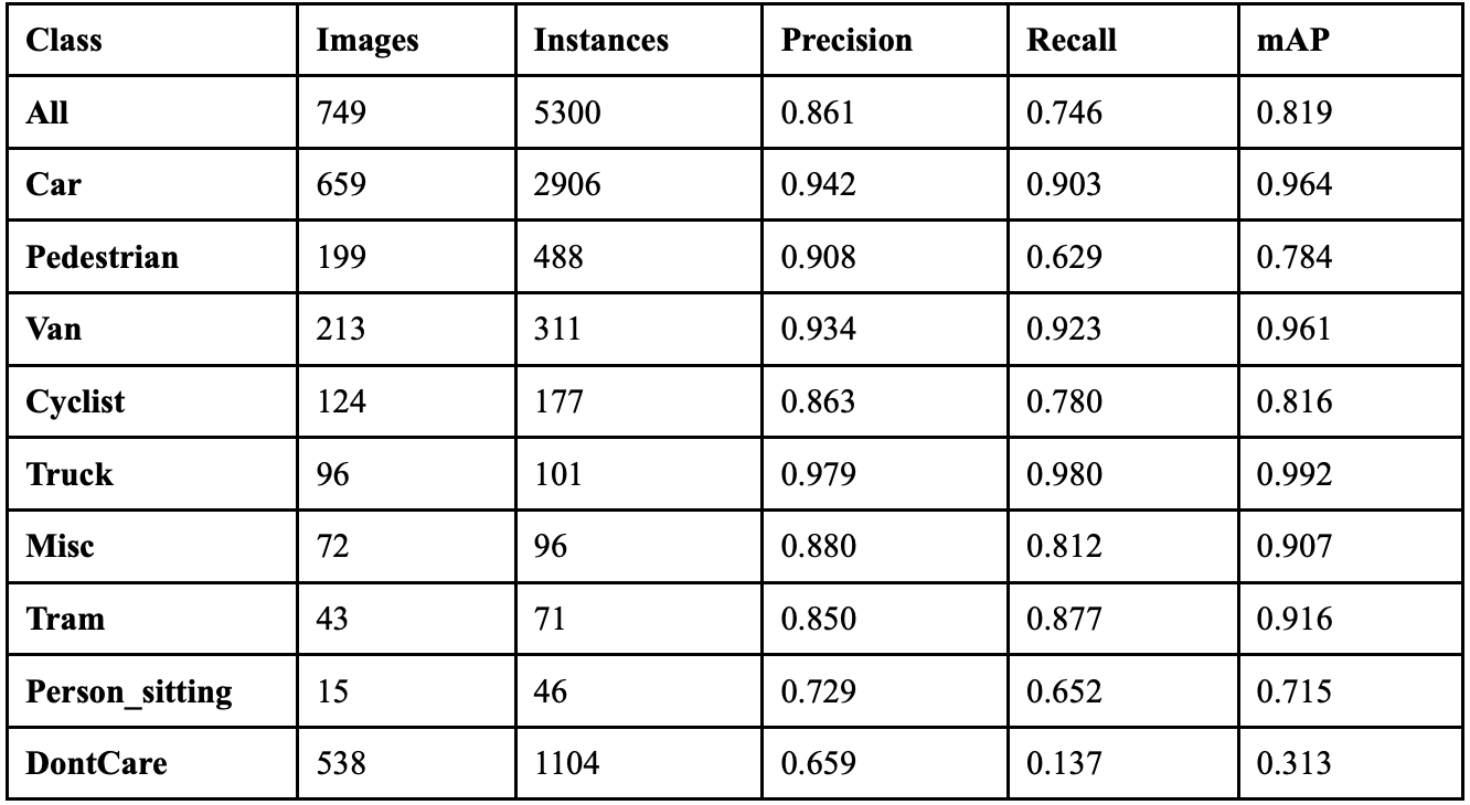
YOLOv8 achieved an overall precision of 86.1%, a recall of 74.6%, a mAP50 of 81.9%, and a mAP50-95 of 59.2%. The YOLOv8 model took 2.805 hours to train on its 100 epochs, and resulted in an F1 score of 0.799. Table 2 shows the class-wise performance of YOLOv8. The model exhibits severe object deletion syndrome, erasing 899 real objects while creating only 395 phantom objects, resulting in a net destruction of 504 visual objects from scenes. The widespread object disappearance suggests YOLOv8’s anchor-free detection head successfully identifies objects, but the model loses confidence during final classification, causing detected objects to be reclassified as background due to overly conservative confidence thresholds. The technical issues stem from YOLOv8’s NMS implementation over-suppressing valid detections while simultaneously allowing false positives to persist, indicating poor calibration of IoU thresholds and the split Ultralytics head’s confidence scoring mechanism.

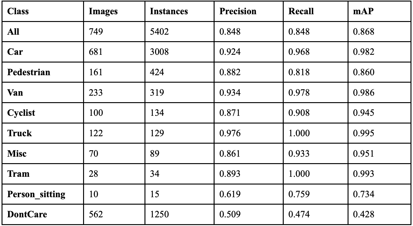
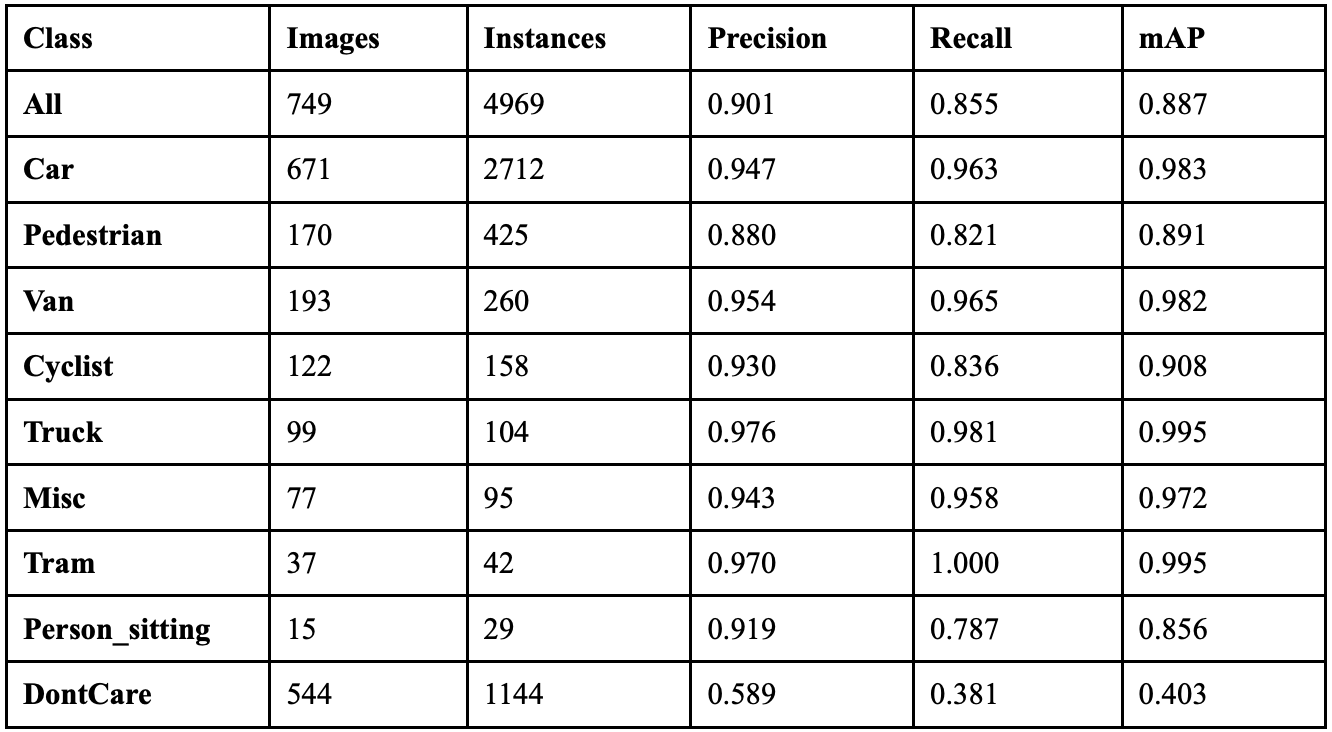
YOLOv9 achieved an overall precision of 84.8%, a recall of 84.8%, a mAP50 of 86.8%, and a mAP50-95 of 69.6%. The YOLOv9 model took 9.468 hours to train on its 100 epochs, and resulted in an F1 score of 0.848. Table 3 shows the class-wise performance of YOLOv9. The model’s PGI mechanism successfully addresses information bottleneck problems for most object categories, with 6 classes showing less than 10% erasure rates, indicating strong information preservation during forward propagation. YOLOv9’s GELAN architecture proves highly efficient with 4 classes, achieving less than 90% identity stability.

Despite these improvements, the model maintains conservative classification behavior with certain challenging classes, like Person_sitting, while creating only 197 phantom objects. This suggests YOLOv9 balances precision and recall effectively in its detection pipeline.

YOLOv10 achieved an overall precision of 80.1%, a recall of 74.6%, a mAP50 of 80.3% and a mAP50-95 of 58.5%. The YOLOv10 model took 3.219 hours to train on its 100 epochs, and resulted in an F1 score of 0.773. Table 4 shows the class-wise performance of YOLOv10. The model achieved 3,821 correct object detections, but predicted 453 phantom objects and did not detect 597 objects. The efficiency benefits offered by YOLOv10’s elimination of NMS come at the cost of worsened precision and recall. This model performed the worst out of all models tested, suggesting NMS is needed for object detection consistency and accuracy.

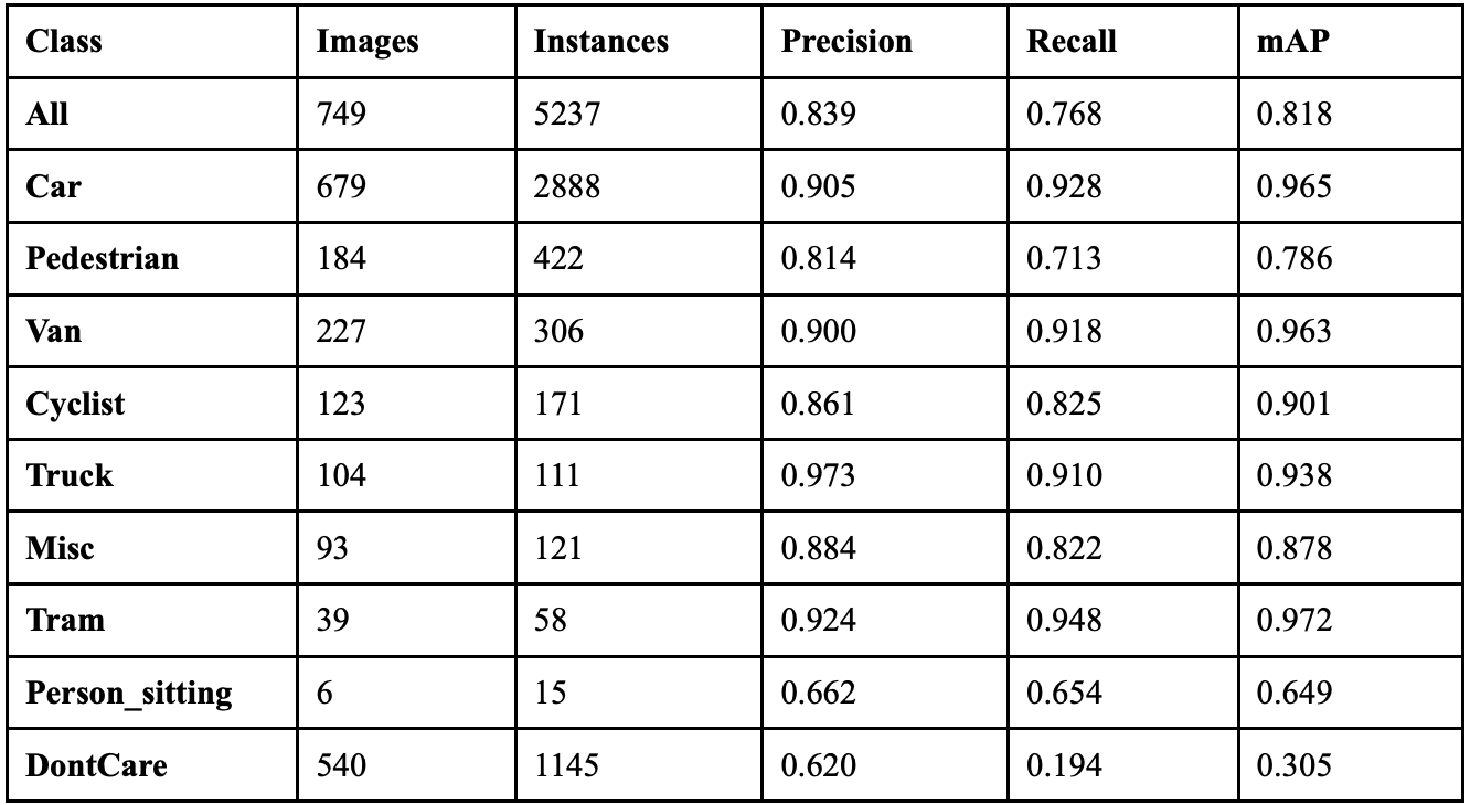
YOLOv11 achieved an overall precision of 83.9%, a recall of 76.8%, a mAP50 of 81.8% and a mAP50-95 of 60.9%. The YOLOv11 model took 3.227 hours to train on its 100 epochs, and resulted in an F1 score of 0.802. Table 5 shows the class-wise performance of YOLOv11. The model correctly predicts 4,817 objects, but decreases, erases 928, and predicts 339 phantom objects. This model struggles most with background detection and differentiating between different types of vehicles. 38 cars are classified as background objects, and 10 cars are classified as vans. This suggests YOLOv11 prioritizes computational efficiency over feature discrimination, resulting in the model being unable to distinguish between similar object classes.

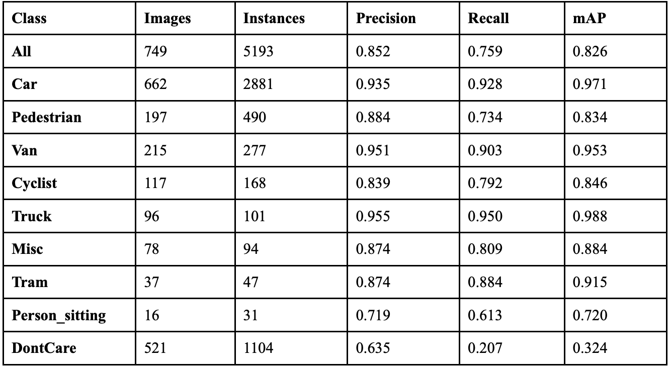
YOLOv12 achieved an overall precision of 85.2%, a recall of 75.9%, a mAP50 of 82.6% and a mAP50-95 of 60.6%. The YOLOv12 model took 3.269 hours to train on its 100 epochs, and resulted in an F1 score of 0.803. Table 6 shows the class-wise performance of YOLOv12. The model correctly predicts 4,779 objects, while erasing 795 and creating 331. The model’s performance is very class-dependent, with only 3 classes achieving less than 15% erasure rates. The model simultaneously over-attends to background regions while under-attending to real objects, similarly to most of the other YOLO models tested. 152 phantom cars are predicted, 102 phantom pedestrians are predicted, 35 cars are classified as background, 10 DontCare instances are classified as cars, and 6 cars are classified as pedestrians. This suggests that YOLOv12’s attention-centric architecture fails to solve the object detection problems encountered in previous models, like YOLOv11.

Table 7 displays the overall performance of each YOLO model together. YOLOv8 achieved the highest precision, but did not perform exceptionally well in recall.

YOLOv9 achieved the highest recall while maintaining a high precision, so it attained the highest F1 score. The models that performed the next best were YOLOv12 and YOLOv11, both achieving F1 scores 0.045 and 0.044 lower than YOLOv9, respectively. The median latency is 2.55 milliseconds per image. Despite its exceptional performance, YOLOv9’s latency is almost three times as much as this median. The models that provide a more balanced ratio of latency and performance are YOLOv11 and YOLOv12. All six models show similar class-wise trends. Each model performs best on larger objects, like trucks, cars, and vans. Smaller objects like people and cyclists have the worst performances. Every model’s best performing class is:

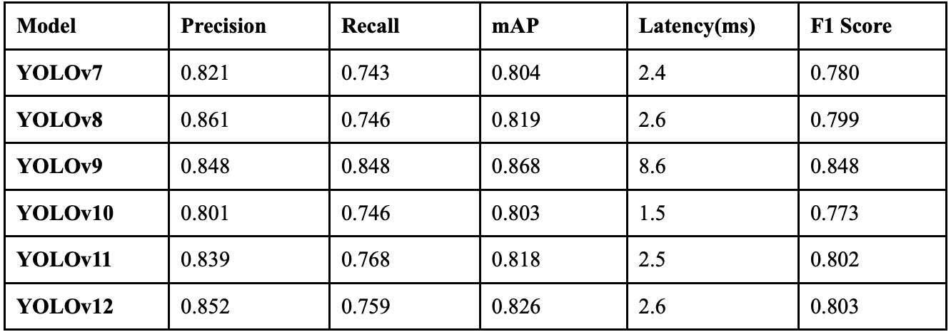
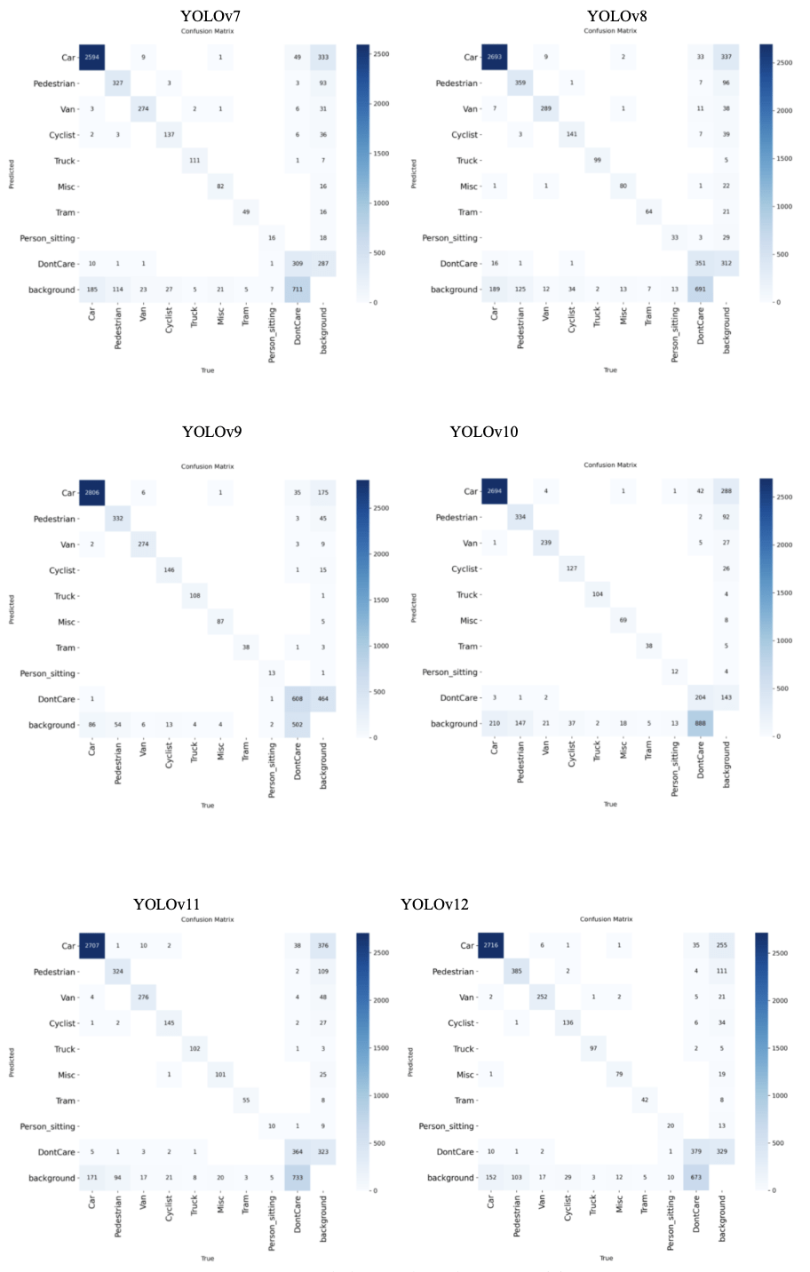
Truck, while their worst performing class is Person_sitting. Fig. 10 displays the confusion matrices for the 6 models, and Fig. 11 depicts sample prediction images from YOLOv9.

Impact of Data Augmentation Techniques

Effect of Mixup Augmentation

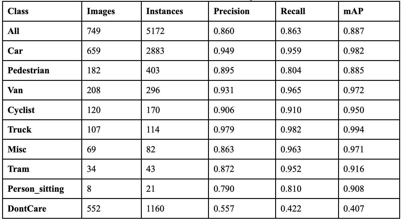
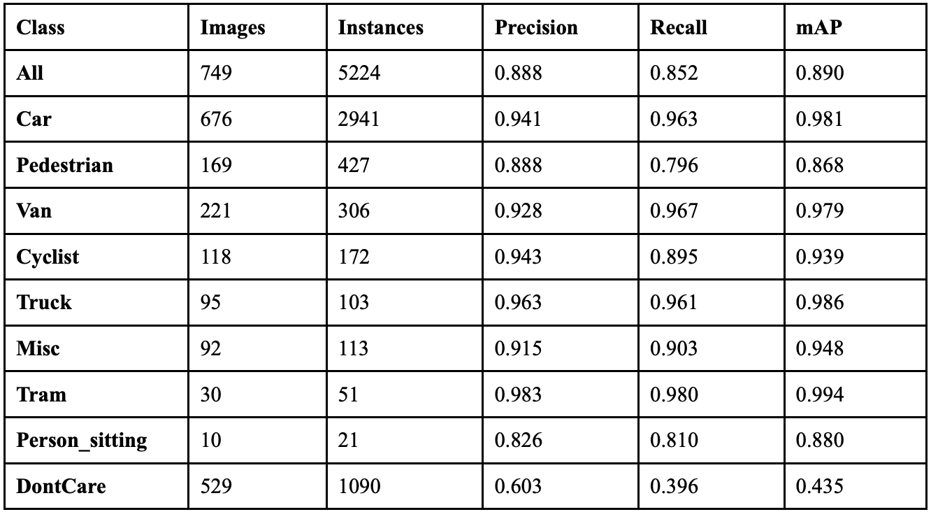
When YOLOv9 ran with a mixup augmentation coefficient of 0.1, it achieved an overall precision of 89.3%, a recall of 86.0%, a mAP50 of 89.6%, a mAP50-95 of 71.5%, and a F1 score of 0.876. This implementation of mixup showed a 4.5% increase in precision, a 1.2% increase in recall, and an improvement in F1 score of .28. Table 8 shows the class-wise performance of implementing mixup at this value. The non-vehicle classes saw major improvements in precision: Person_sitting increased by 23.1%, Pedestrian increased by 3.2%, and Cyclist increased by 4.8%. The recall for the Truck and Van classes dropped by 3.6% and 2.0% respectively, yet both classes’ recalls remained over 95% When the model ran with a mixup coefficient of 0.3, it achieved an overall precision of 89.8%, a recall of 83.0%, a mAP50 of 88.7%, a mAP50-95 of 71.8%, and a F1 score of 0.863.

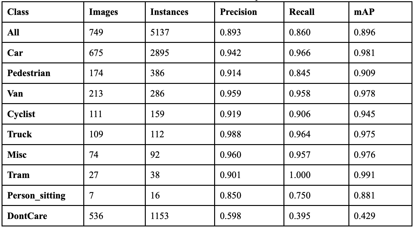
Table 9 shows the class-wise performance of implementing mixup at this value. While the overall performance dropped when increasing the mixup to 0.3, the Pedestrian class saw improvements. The precision of this class improved by 1.5% and the model achieved 404 correct detections. However, the Cyclist class dropped in precision by 4.0% and background confusion increased. Across several classes, there were more false positives than before, suggesting the higher mixup coefficient may be making the model too conservative in certain cases.

When the model ran with a mixup coefficient of 0.5, it achieved an overall precision of 88.7%, a recall of 86.8%, a mAP50 of 89.2%, a mAP50-95 of 71.3%, and a F1 score of 0.877. Table 10 shows the class-wise performance of implementing mixup at this value. Overall performance increased compared to the last two experiments. The classes that benefited from the new mixup coefficient the most were the vehicle classes: Car, Van, and Truck. Person_sitting also saw major improvements, as it achieved 29 correct predictions, 20 more than the model did without augmentation. The Cyclist class, however, had a drop in recall with minimal improvement in precision, and background false positives also decreased.

When the model ran with a mixup coefficient of 0.7, it achieved an overall precision of 86.0%, a recall of 86.3%, a mAP50 of 88.7%, a mAP50-95 of 71.3%, and a F1 score of 0.861. Table 11 shows the class-wise performance of implementing mixup at this value. When increasing the augmentation to 0.7, there was an overall decline; however, some classes still saw improvements. The classes that peaked with this implementation were Cyclist, with 157 correct predictions, and Tram, with 42 correct predictions. Every other class saw regression, with Pedestrian having its worst performance in this experiment. This implementation also resulted in increased background confusion, as the model is getting less confident about what instances are objects or backgrounds.

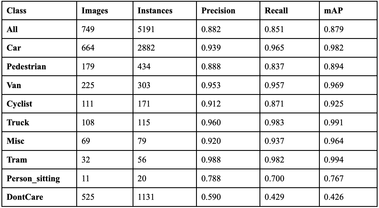
When the model ran with a mixup coefficient of 0.9, it achieved an overall precision of 88.9%, a recall of 86.7%, a mAP50 of 89.2%, a mAP50-95 of 72.4%, and a F1 score of 0.878. Table 12 shows the class-wise performance of implementing mixup at this value. The classes that peaked in this implementation were Truck, Car, Van, and Cyclist. While they did not peak in this experiment, other classes still had far better performance than they did when no augmentation was applied to the model. This implementation also resulted in reduced background confusion, suggesting the model is getting more confident in identifying objects.

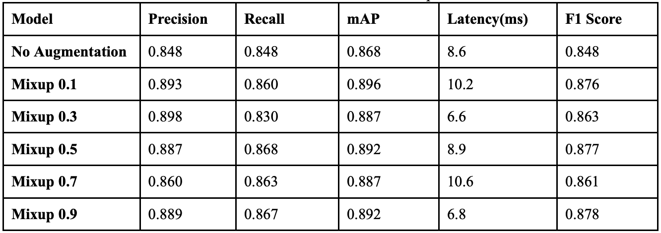
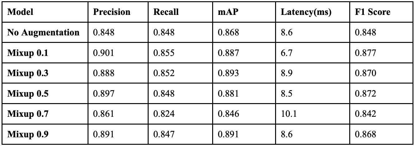
Table 13 displays the overall performance of each mixup coefficient together. When the coefficient was 0.1, the model achieved the highest precision, and when it was implemented at 0.5, it achieved its highest recall. When the coefficient was 0.9, it struck a better balance between precision and recall, resulting in the highest F1 score.

Compared to when the model had no augmentation, implementing mixup at 0.9 resulted in a 4.1% increase in precision, a 1.9% increase in recall, and a F1 score increase of 0.030, a considerable improvement. All classes benefited from the augmentation, but the non-vehicle classes benefited the most. The Person_sitting, Pedestrian, and Cycling classes all saw substantial improvements when subjected to severe augmentation, while the Car, Truck, and Van classes saw minimal improvements. Since the non-vehicle classes are less frequent in the dataset and contain smaller objects, this suggests that mixup augmentation helps improve precision and recall on instances that show up less frequently or are smaller. Fig. 12 displays the confusion matrices for all implementations of mixup.

Effect of Cutmix Augmentation

When YOLOv9 ran with a cutmix coefficient of 0.1, it achieved an overall precision of 90.1%, a recall of 85.5%, a mAP50 of 88.7%, a mAP50-95 of 70.9%, and a F1 score of 0.877. Table 14 shows the class-wise performance of implementing cutmix at this value. The non-vehicle classes saw major improvements in precision: Person_sitting increased by 30.0%, Pedestrian remained stable with a slight decline of 0.2%, and Cyclist increased by 5.9%. Person_sitting achieved 19 correct detections, more than doubling from 9 with no augmentation. Background confusion decreased significantly across most classes, with 122 fewer total background misclassifications compared to no augmentation.

When the model ran with a cutmix coefficient of 0.3, it achieved an overall precision of 88.8%, a recall of 85.2%, a mAP50 of 89.0%, a mAP50-95 of 71.6%, and a F1 score of 0.870. Table 15 shows the class-wise performance of implementing cutmix at this value. This augmentation level achieved the highest mAP50 score across all cutmix coefficients. The Pedestrian class saw significant improvements, achieving 369 correct detections compared to 344 with no augmentation, representing a 7.3% increase. Person_sitting maintained its improved performance with 19 correct detections. However, some vehicle classes, like Van, showed slight performance decreases compared to lighter augmentation levels.

When the model ran with a cutmix coefficient of 0.5, it achieved an overall precision of 88.2%, a recall of 85.1%, a mAP50 of 87.9%, a mAP50-95 of 71.3%, and a F1 score of 0.866. Table 16 shows the class-wise performance of implementing cutmix at this value. Performance began to decline compared to lighter augmentation levels, though it still maintained improvements over no augmentation. Person_sitting dropped to 14 correct detections, showing sensitivity to higher cutmix coefficients. Vehicle classes remained relatively stable, with Car maintaining 98.2% mAP50. Background confusion increased slightly compared to 0.1 and 0.3, with 67 fewer background misclassifications than with no augmentation.

When the model ran with a cutmix coefficient of 0.7, it achieved an overall precision of 85.2%, a recall of 82.7%, a mAP50 of 85.1%, a mAP50-95 of 68.8%, and a F1 score of 0.839. Table 17 shows the class-wise performance of implementing cutmix at this value. This represented the worst overall performance across all cutmix values, with significant declines in most metrics. Person_sitting performance collapsed to just 4 correct detections with 53.4% mAP50, suggesting over-augmentation. However, some classes, like Truck, achieved a perfect 100% recall, and Tram maintained strong performance with 99.5% mAP50. Background confusion patterns remained similar to 0.5, but the overall detection confidence decreased substantially.

When the model ran with a cutmix coefficient of 0.9, it achieved an overall precision of 86.6%, a recall of 86.9%, a mAP50 of 89.1%, a mAP50-95 of 71.2%, and a F1 score of 0.867. Table 18 shows the class-wise performance of implementing cutmix at this value. Performance recovered significantly from the 0.7 dip, showing the highest recall across all cutmix values. Person_sitting achieved remarkable recovery with 19 correct detections and 94.0% mAP50, its best performance across all augmentation levels. The model achieved the best balance between precision and recall at this extreme augmentation level. Background confusion decreased by 94 fewer misclassifications than with no augmentation, suggesting improved object-background distinction.

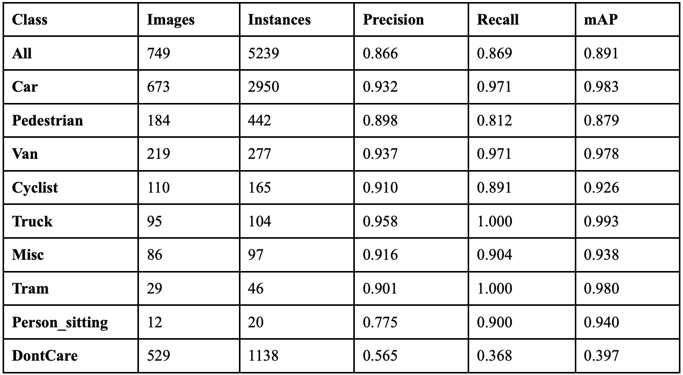
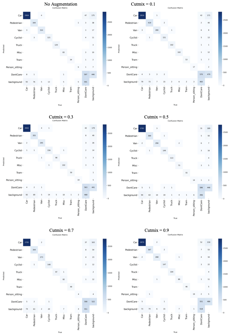
Table 19 displays the overall performance of each cutmix value together. When cutmix was implemented at 0.1, the model achieved the highest precision at 90.1%, and when implemented at 0.9, it achieved the highest recall at 86.9%. The model achieved the highest mAP50 of 89.0% at cutmix 0.3, while cutmix 0.1 resulted in the highest F1 score of 0.877. Compared to when the model had no augmentation, implementing cutmix at 0.1 resulted in a 7.1% increase in precision, though with a 1.6% decrease in recall, and a F1 score increase of 0.027. All classes benefited from cutmix augmentation, but the non-vehicle classes benefited the most dramatically. The Person_sitting class showed the most substantial improvements, achieving over double the correct detections with cutmix compared to no augmentation. Since the non-vehicle classes are less frequent in the dataset and contain smaller objects, this suggests that cutmix augmentation particularly helps improve performance on instances that show up less frequently or are smaller, likely due to the occlusion-based training that cutmix provides. Fig. 13 displays the confusion matrices for all implementations of cutmix.

Conclusions and Future Work

In this paper, we set out to improve object detection models for car safety features to reduce the number of accidents and fatalities that occur on roads. To do this, we compared 6 different YOLO models and investigated how we can improve them with data augmentation schemes. It was found that the model that achieved the highest overall performance was YOLOv9, which achieved a precision of 84.8%, a recall of 84.8%, and an F1 score of 84.8%. Implementing a mixup factor of 0.9 and a cutmix factor of 0.1 improved the performance of the model the most. The mixup factor of 0.9 improves the model’s precision by 4.1% and its recall by 1.9%, resulting in a F1 score increase of 3.0%. The cutmix factor of 0.1 increases the model’s precision by 5.3% and its recall by 0.7%, resulting in a F1 score increase of 2.9%.

Our objective of determining the most accurate object detection and classification model, and finding the best ways to improve it, was achieved: To attain the highest accuracy and precision when detecting roadside objects, YOLOv9 must be used with a mixup factor of 0.9 or a cutmix factor of 0.1. The implementation of this more precise and accurate model could transform automotive safety standards. It provides drivers with enhanced awareness of their surroundings, instead of relying on their reaction times and potentially impaired judgment. This will heavily reduce car accidents and injuries, allowing drivers to feel safer in their cars.

Several areas can be investigated further. First, the work can be extended to include other object detection models alongside YOLO. Second, more training parameters other than augmentation schemes can be used to improve the model. Third, real-time object detection devices can be built into vehicles using improved models to help prevent accidents and fatalities. There were also several limitations in this study. First, the study’s scope was constrained to controlled dataset conditions without accounting for environmental variables like fog, rain, or nighttime scenarios that commonly affect real-world driving. Additionally, performance evaluation relied on standard metrics without considering edge cases or failure modes that could prove critical in actual deployment scenarios. The next critical step is transitioning these laboratory findings into production vehicles, where this optimized object detection system could significantly reduce the 1.2 million annual traffic fatalities caused by delayed driver reactions.

References

1. Road traffic injuries. (2023, December 13). World Health Organization (WHO). Retrieved July 16, 2025, from https://www.who.int/news-room/fact-sheets/detail/road -traffic-injuries [↩]
2. U.S. Department of Transportation & National Highway Traffic Safety Administration. (2017, October). 2016 Fatal Motor Vehicle Crashes: Overview. https://crashstats.nhtsa.dot.gov/Api/Public/ViewPublication/812456 [↩]
3. Winland, V. (2025, March 6). What Is Feature Extraction? IBM. https://www.ibm.co m/think/topics/feature-extraction [↩]
4. Li, K., Ma, W., Sajid, U., Wu, Y., & Wang, G. (2019). Object Detection with Convolutional Neural Networks. ArXiv. https://arxiv.org/abs/1912.01844 [↩]
5. Geiger, A., Lenz, P., Stiller, C., & Urtasun, R. (2013). Vision meets robotics: The KITTI dataset. International Journal of Robotics Research, 32(11), 1231-1237. https://www.cvlibs.net/datasets/kitti/ [↩]
6. Yang, S., Xiao, W., Zhang, M., Guo, S., Zhao, J., & Shen, F. (2022). Image Data Augmentation for Deep Learning: A Survey. ArXiv. https://arxiv.org/abs/2204.08610 [↩]
7. Chen, W., Yan, J., Huang, W., et al. (2024). Robust object detection for autonomous driving based on semi-supervised learning. Security and Safety, 3, 2024002. https://sands.edpsciences.org/articles/sands/full_html/2024/01/sands20230024/ [↩]
8. Sahoo, L. K., & Varadarajan, V. (2025). Deep learning for autonomous driving systems: technological innovations, strategic implementations, and business implications – a comprehensive review. Complex Engineering Systems, 5, 2. https://doi.org/10.20517/ces.2024.83 [↩]
9. Zhao, Y., Lv, W., Xu, S., Wei, J., Wang, G., Dang, Q., Liu, Y., & Chen, J. (2023). DETRs Beat YOLOs on Real-time Object Detection. ArXiv. https://arxiv.org/abs/2304.08069 [↩]
10. Vu, T., Sun, B., Yuan, B., Ngai, A., Li, Y., & Frahm, J. (2023). Supervision Interpolation via LossMix: Generalizing Mixup for Object Detection and Beyond. ArXiv. https://arxiv.org/abs/2303.10343 [↩]
11. Zhao, H., Sheng, D., Bao, J., Chen, D., Chen, D., Wen, F., Yuan, L., Liu, C., Zhou, W., Chu, Q., Zhang, W. & Yu, N.. (2023). X-Paste: Revisiting Scalable Copy-Paste for Instance Segmentation using CLIP and StableDiffusion. Proceedings of the 40th International Conference on Machine Learning, in Proceedings of Machine Learning Research 202:42098-42109 Available from https://proceedings.mlr.press/v202/zhao23f.html [↩]
12. Jia, X., Tong, Y., Qiao, H., et al. (2023). Fast and accurate object detector for autonomous driving based on improved YOLOv5. Scientific Reports, 13, 9711. https://doi.org/10.1038/s41598-023-36868-w [↩]
13. Zhou, Y., Wen, S., Wang, D., Meng, J., Mu, J., & Irampaye, R. (2022). MobileYOLO: Real-Time Object Detection Algorithm in Autonomous Driving Scenarios. Sensors (Basel, Switzerland), 22(9), 3349. https://doi.org/10.3390/s22093349 [↩]
14. Wei, J., As’arry, A., Anas Md Rezali, K., Zuhri Mohamed Yusoff, M., Ma, H., & Zhang, K. (2025). A review of YOLO algorithm and its applications in autonomous driving object detection. IEEE Access, 13, 93688-93711. https://doi.org/10.1109/ACCESS.2025.3573376 [↩]
15. Redmon, J., Divvala, S., Girshick, R., & Farhadi, A. (2015). You Only Look Once: Unified, Real-Time Object Detection. ArXiv. https://arxiv.org/abs/1506.02640 [↩]
16. Jocher, G., & Keita, Z., 2024, September 28. YOLO Object Detection Explained. DataCamp. https://www.datacamp.com/blog/yolo-object-detection-explained [↩]
17. Kindu, R. (2023, January 17). YOLO: Algorithm for Object Detection Explained [+Examples]. V7 Labs. https://www.v7labs.com/blog/yolo-object-detection [↩]
18. Wang, C., Bochkovskiy, A., & Liao, H. (2022). YOLOv7: Trainable bag-of-freebies sets new state-of-the-art for real-time object detectors. ArXiv. https://arxiv.org/abs/220 7.02696 [↩]
19. Boesch, G. (2023, November 21). YOLOv7: A Powerful Object Detection Algorithm- viso.ai. Viso Suite. https://viso.ai/deep-learning/yolov7-guide/ [↩]
20. Reis, D., Kupec, J., Hong, J., & Daoudi, A. (2023). Real-Time Flying Object Detection with YOLOv8. ArXiv. https://arxiv.org/abs/2305.09972 [↩]
21. Wang, C., Yeh, I., & Liao, H. (2024). YOLOv9: Learning What You Want to Learn Using Programmable Gradient Information. ArXiv. https://arxiv.org/abs/2402.13616 [↩]
22. Wang, A., Chen, H., Liu, L., Chen, K., Lin, Z., Han, J., & Ding, G. (2024). YOLOv10: Real-Time End-to-End Object Detection. ArXiv. https://arxiv.org/abs/2405 .14458 [↩]
23. Khanam, R., & Hussain, M. (2024). YOLOv11: An Overview of the Key Architectural Enhancements. ArXiv. https://arxiv.org/abs/2410.17725 [↩]
24. Tian, Y., Ye, Q., & Doermann, D. (2025). YOLOv12: Attention-Centric Real-Time Object Detectors. ArXiv. https://arxiv.org/abs/2502.12524 [↩]