Tree Seedlings Survival Prediction Using Machine Learning Under Class Imbalance

Leyla Bashirova¹, Abdulla Kerimov^2
1 College du Leman International School, Switzerland
² Stanford University PhD Alumni, Houston, TX, USA

Abstract

Most studies on tree seedlings survival evaluate plant–soil feedbacks, functional traits, microbial dynamics, and environmental effects in isolation. We present a case study using a single controlled experimental dataset (one season; four species; seven soils) to evaluate how well machine learning models can predict seedling survival. We tested multiple algorithms (Random Forest, XGBoost, KNN, and Logistic Regression) and compared different class-imbalance approaches: class weighting, undersampling, and oversampling. Under class weighting, minority-class (Alive) performance was uneven across algorithms, with Logistic Regression, KNN, and XGBoost achieving similar Alive test F1 scores (~52–54%) while Random Forest performed best (Alive test F1 = 62.3% ±6.6%) and also led ROC AUC and PR AUC. The undersampling approach reduced differences between the strongest models, with Random Forest and XGBoost becoming statistically not significant in accuracy, although absolute minority-class gains were modest. The oversampling technique, ADASYN, resulted in the strongest overall minority-class performance, particularly, for XGBoost (Alive test F1 = 61.6% ±8.1%; Alive PR AUC = 54.1% ±9.7%).  The ADASYN showed the clear performance differences between the models and increased the algorithm-specific differences.  SHAP-based feature importance analysis identified phenolics, lignin, non-structural carbohydrates (NSC), and arbuscular mycorrhizal fungi (AMF) as the strongest contributors to model predictions. This supports ecological theory emphasizing chemical defense, tissue repair capacity, and mutualistic pathogen protection. While our findings are limited to this case study and their generalization to other forests, soils, species, and time remains to be tested. We found that machine learning paired with an imbalance technique can help generate testable predictions of seedling outcomes for reforestation and forest management contexts.

Keywords: Tree seedlings, environment, light, function traits, conditions, survival, machine learning, model tuning, confidence intervals, oversampling, SHAP analysis

Introduction

Tree survival prediction is essential for both global and ecological sustainability. Trees play an important role in maintaining biodiversity, regulating climate change, and supporting life on Earth. Predicting if tree seedlings will survive under different environmental conditions, such as soil type, soil chemical and physical properties, nutrient availability, and light exposure, is key for understanding how forests respond to environmental conditions. By understanding and modeling these relationships, we can potentially assess the impacts of climate change, deforestation, and soil degradation on forest dynamics¹. Predicting tree seedlings survival helps with understanding shifts in forest composition and health, guide reforestation and assist migration efforts. It also can inform conservation strategies, and support ecosystem resilience. Overall, being able to predict tree seedlings survival can allow scientists and land managers to make informed decisions that protect the environment and forest ecosystems.

Tree seedling survival is impacted by complex biotic and abiotic factors. They interact at different spatial and biological scales. Seedlings experience some of the highest mortality rates within a tree’s life cycle. Therefore, early survival prediction is important in tree population persistence and forest structure. Environmental constraints such as moisture stress, nutrient limitation, and light availability can strongly affect a seedling’s survival rate. Also, biotic interactions, such as competition with neighboring plants, colonization by beneficial fungi, or exposure to pathogens, can fundamentally change survival outcomes. Understanding how these different factors together impact survival has therefore become a key goal in ecology, restoration, and forest management. However, despite extensive research in ecology, predicting survival of tree seedlings remains challenging because they respond nonlinearly to environmental conditions and biological interactions. These relationships often vary between different species and soil type, and growing conditions.

As global forests are affected by climate change, invasive species, and anthropogenic disturbance, there is a need for tools that can predict survival under different conditions. Machine learning offers a potential solution. It can integrate large numbers of environmental and biological variables, capture nonlinear interactions, and identify complex patterns that are difficult to detect with traditional approaches. Developing such predictive models is critical for reforestation and conservation planning, where practitioners must decide which species and where to plant them. Most importantly to identify the environmental conditions that can help plants to grow and thrive. By combining ecological understanding with data science, predictive modeling can help us to manage forests, enhance ecosystem resilience, and mitigate future biodiversity loss.

Relevant Works

Extensive work in ecological research aims to understand the key factors affecting tree seedling survival. Survival outcomes are based on the plant–soil feedbacks (PSFs), functional traits, microbial communities, and environmental conditions. Plant–soil feedbacks are a key mechanism affecting seedling growth. This includes when plants modify soil biotic and abiotic properties in ways that influence plant growth^2,3,4,5,6. These feedback loops, first articulated by⁷, can influence biodiversity and ecosystem functions. Soil-borne microbes, such as fungi and pathogenic organisms, are key agents of PSFs^8,9.

Within these microbial communities, Arbuscular Mycorrhizal Fungi (AMF) play a particularly significant role by forming mutualistic relationships with seedlings, exchanging nutrients and water for photosynthates¹⁰. Mycorrhizal colonization is often higher in conspecific soils and soils containing adult trees of the same mycorrhizal type, therefore affecting seedling growth^11,12,13. AMF can indirectly suppress pathogens¹⁴, while ectomycorrhizal fungi (EMF) provide physical protection to roots¹⁵.

Functional traits, such as physiological or structural attributes, impact survival by influencing stress tolerance, defense, and recovery¹⁶. Key traits such as phenolics, lignin, and non-structural carbohydrates (NSC) relate directly to chemical defense, structural integrity, and energy storage^17,18,19. Their impact depends on soil type, microbial composition, and nutrient availability^20,21,22,23.

Environmental factors, such as light availability, can change both PSFs and functional traits^24,25. Light controls microbial abundance^26,27, increases AMF activity^28,29, and influences both seedling and pathogen mortality^30,31,32. Light also affects the amount of phenolics and lignin^33,34,35.

Recent work in literature attempted to apply computational tools to include these different effects. Wood et al. (2023) explored the use of Cox proportional hazards models to predict seedling survival. They identified light availability, species types, and carbon reserves as key contributors³⁶. Together, these studies demonstrate that seedling survival is the result of complex biotic and abiotic interactions that change between different species, soils, and environmental conditions.

Research Gap and Contribution

Many existing studies about tree seedling survival focus on investigating individual factors, such as PSFs, functional traits, or light-driven microbial dynamics, in isolation. These studies provide important insights but are not able to capture the nonlinear, complex interactions between different factors that affect the survival outcomes. Traditional statistical models, such as the Cox proportional hazards model, assume linearity that simplifies ecological processes. As a result, they may overlook nonlinear patterns from simultaneous interactions among different factors such as soil microbes, plant traits, nutrient availability, and environmental variability. 

This creates a clear methodological gap. There is a need for integrated, data-driven predictive frameworks capable of handling complex interactions and high-dimensional inputs. Machine learning models are well-suited to this challenge because they can capture nonlinear relationships, capable of processing multiple variable types, and identify important predictors of survival. While recent efforts include exploring the machine learning based tools, the application of machine learning to seedling survival remains limited and underdeveloped.

To address this gap, our study evaluates multiple machine learning algorithms to predict seedling survival across varying soil, microbial, and environmental conditions.  Our work contributes by (1) integrating multiple ecological drivers into a single predictive model, (2) identifying which modeling strategies best capture minority-class survival patterns, and (3) demonstrating how machine learning can complement ecological theory to improve forecasting of seedling outcomes. Our combined ecological and computational approach can strengthen the efforts to support reforestation, forest management, and climate adaptation planning.

Dataset

In this study, we used a tree seedlings survival dataset from Woods et al. 2023 [36]. They conducted experiments, using a factorial blocked design with four tree species, seven soil types, and different light conditions, to understand how tree seedling functional traits influence survival in different conditions. Overall, there are 3,024 seedlings data has been collected.

The seedlings were monitored twice a week throughout a growing season. At three weeks, they would randomly select groups of seedlings to measure for mycorrhizal colonization, phenolics, lignin, and NSC. They measured how much fungi would be on the seed or soil, how many chemicals in the plant to keep it healthy, how many chemicals on the cell wall to keep it strong and stable, and lastly carbohydrates that are not a part of the plant to help it grow and have energy. Wood et al., (2023) suggested that seedling traits could have an important role in mediating the effects of local solid source and light levels on seedling survivorship and thus plant traits could have an important role in plant-soil feedbacks³⁶. 

The dataset includes information about seed identification and experimental setup, planting and growth dates, tree seedling and soil characteristics, light information, fungal colonization, and biochemical characteristics, and whether or not the seedling survived at the end of growing season as shown in Table 1.  Our target column describes the survival outcome of the planted seedlings. The Alive column indicates if the seedling was alive by the second growing season.

Seed identification  and experimental setup provides identifier and structural information about how the experiment was set up, such as seed identifier, number of  the field plots the seedlings were planted in. The planting and growth timeline describes the time when the seedlings died or was harvested. The Plant date column is the day that seedlings were planted in the field plots. Time column is the number of days passed when the plant died or was harvested. 

Tree seedling and soil characteristics data include information about tree and soil species, soil sterile and conspecific flags.  The species column describes different tree types that include Acer saccharum, Prunus serotina, Quercus alba, and Quercus rubra. Soil column includes all tree species the soil was taken from and Acer rubrum, Populus grandidentata, and a sterilized conspecific for each species. The sterile column indicates if the soil is sterilized or not. Conspecific column indicates if the soil is conspecific, heterospecific, or sterilized conspecific. 

Information about the light exposure of the tree seedlings is another crucial data in this dataset. Light column is the amount of light reaching the plant’s subplot at a height of 1 m. 

The fungal in this experiment is beneficial to the tree and soil. Soil mycro column is the mycorrhizal type of species culturing the soil. Mycro is the mycorrhizal type of seedling species which is either AMF or EMF. AMF is the percent of arbuscular mycorrhizal fungi colonization on the fine roots of harvested seedlings. EMF is the percentage of ectomycorrhizal fungi colonization on the root tips of harvested seedlings. 

Biochemical characteristics data includes  several calculated metrics. The NSC column is calculated as percent dry mass nonstructural carbohydrates (NSC). Lignin column is calculated as percent dry mass lignin. Lastly, the phenolics column is calculated as nmol Gallic acid equivalents per mg dry extract.

Variable Name	Variable Type	Description
Plant date	datetime	Day the seedling was planted in the field plot.
Time	numeric	Number of days when the seedling died or was harvested.
Species	categorical	Different tree species including Acer saccharum, Prunus serotina, Quercus alba, and Quercus rubra.
Soil	categorical	Soil source from Acer saccharum, Prunus serotina, Quercus alba, Quercus rubra, Acer rubrum, Populus grandidentata, or sterilized soil.
Sterile	categorical	Indicates whether the soil was sterilized or not.
Conspecific	categorical	Indicates whether the soil was conspecific, heterospecific, or sterilized conspecific.
Light	numeric	Amount of light reaching each subplot at a height of 1 m.
Soil myco	categorical	Mycorrhizal type (AMF, EMF, or Sterile) of the species used to culture the soil.
Myco	categorical	Mycorrhizal type (AMF or EMF) of the seedling species.
AMF	numeric	Percentage of arbuscular mycorrhizal fungi colonization on the fine roots of harvested seedlings.
EMF	numeric	Percentage of ectomycorrhizal fungi colonization on the root tips of harvested seedlings.
NSC	numeric	Nonstructural carbohydrates, calculated as percent dry mass.
Lignin	numeric	Lignin content, calculated as percent dry mass.
Phenolics	numeric	Phenolic content, calculated as nmol gallic acid equivalents per mg dry extract.
Alive	categorical	Indicates whether the seedling was alive or dead at the end of the first growing season.

Exploratory Data Analysis

In this section, we present the findings from exploratory data analysis. The goal of this analysis is to understand the relationships, patterns, trends, and correlations in the data set. Ultimately, we aim to explore relationships between different input variables with respect to the target variable Alive – whether the seedling was alive at the end of the first growing season.

Figure 1 illustrates count distribution of target variable Alive. It shows an imbalanced distribution of Dead and Alive seedlings. There are 2292 Dead seedlings and 491 Alive seedlings at the end of the growing season. This data imbalance distribution introduces bias towards the majority class, Dead seedlings.

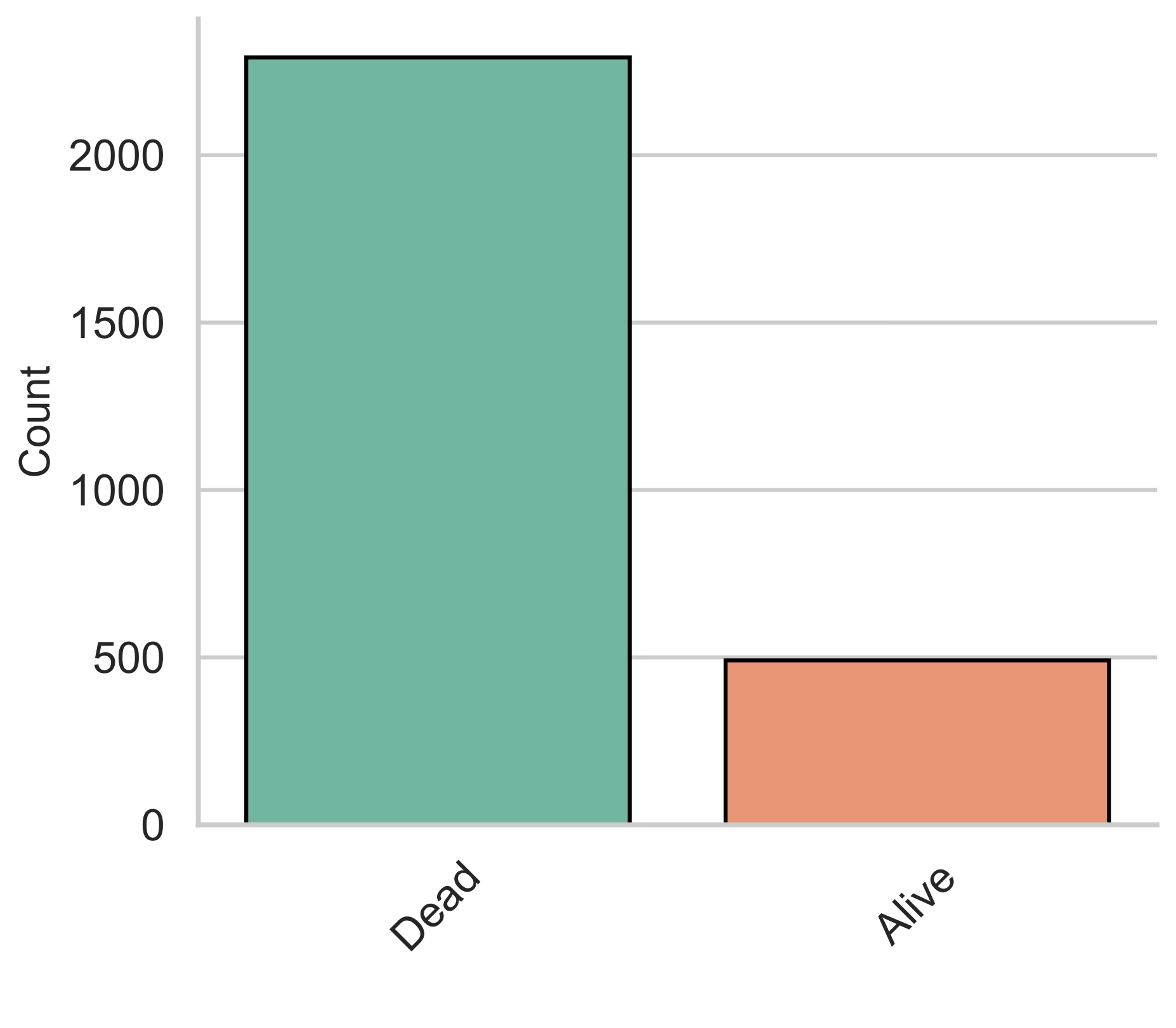
Figure 2 displays the count of Dead or Alive seedlings per species type. It illustrates that the Acer saccharum and Prunus serotina have more Dead seedlings compared to Alive. Quercus alba Quercus Rubra has the most seedlings that live compared to the other types of species. This suggests that Acer saccharum and Prunus serotina seedlings are least likely to survive and Quercus alba Quercus Rubra are more likely to survive at the end of the first growing season.

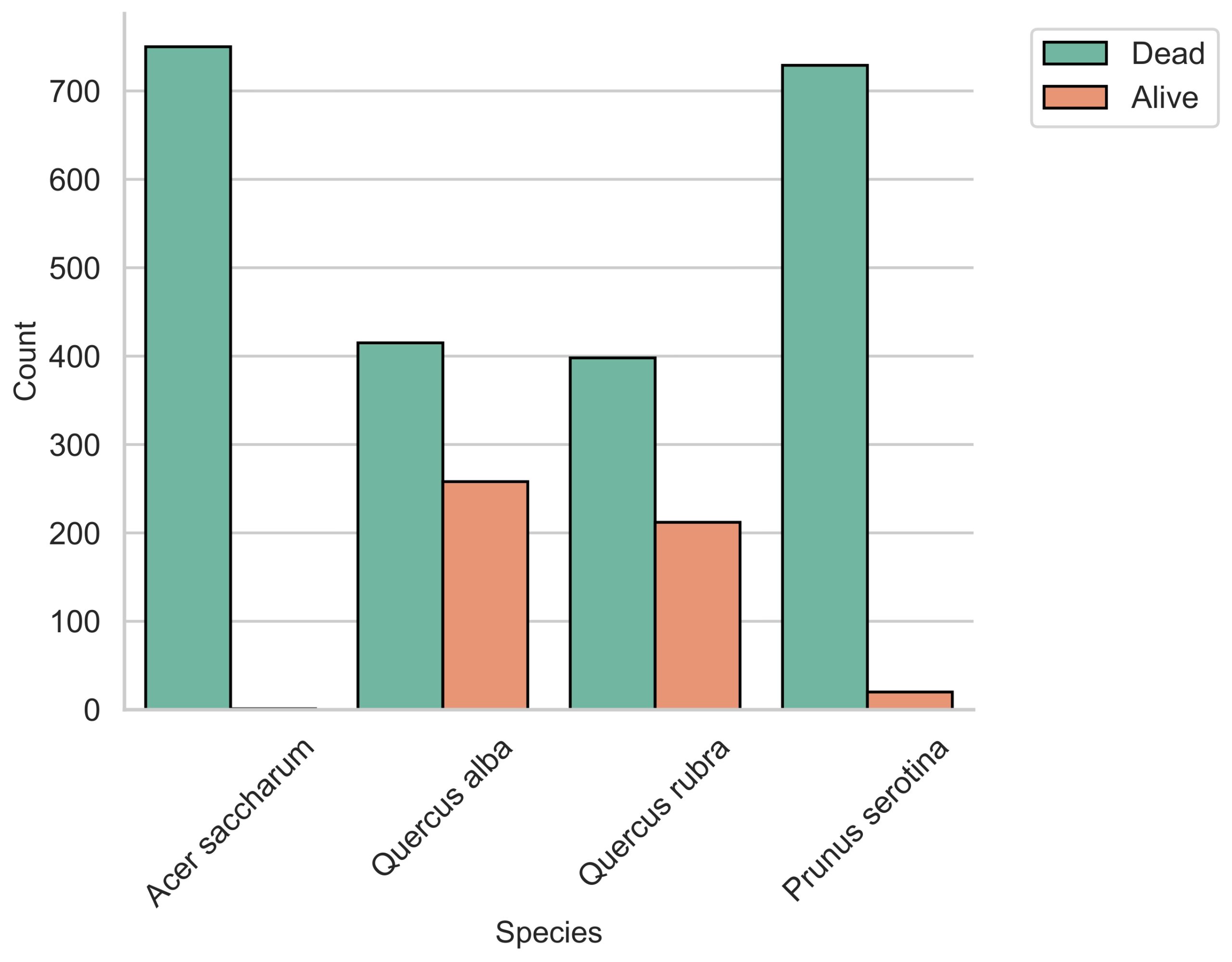
Figure 3 shows the effect of the light on the Dead and Alive seedlings from different species. The median of the light of the Alive seedlings is marginally higher than the one of the Dead seedlings. The 25 and 75 percent tiles of light the distribution of Alive seedlings is slightly different than the ones of Dead seedlings. The interquartile range of the light distribution of Alive seedlings for prunus serotina is the widest compared to the ones of quercus alba. There are few Alive seedlings for the Acer saccharum as shown in Figure 2. 

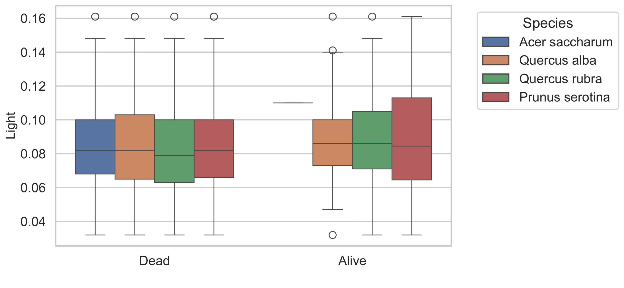
Figure 4 depicts the relationship between phenolics and sterile with respect to the target variable Alive. The median of phenolics for Alive seedlings is significantly larger than the median of phenolics for Dead seedlings. Overall, the median phenolics with non-sterile seedlings is larger than sterile seedlings. Additionally, the phenolics values of non-sterile Alive seedlings are consistently higher than the non-sterile Dead seedlings. This suggests that non-sterile seedlings with high phenolics values are likely to be Alive at the end of the first growing season.

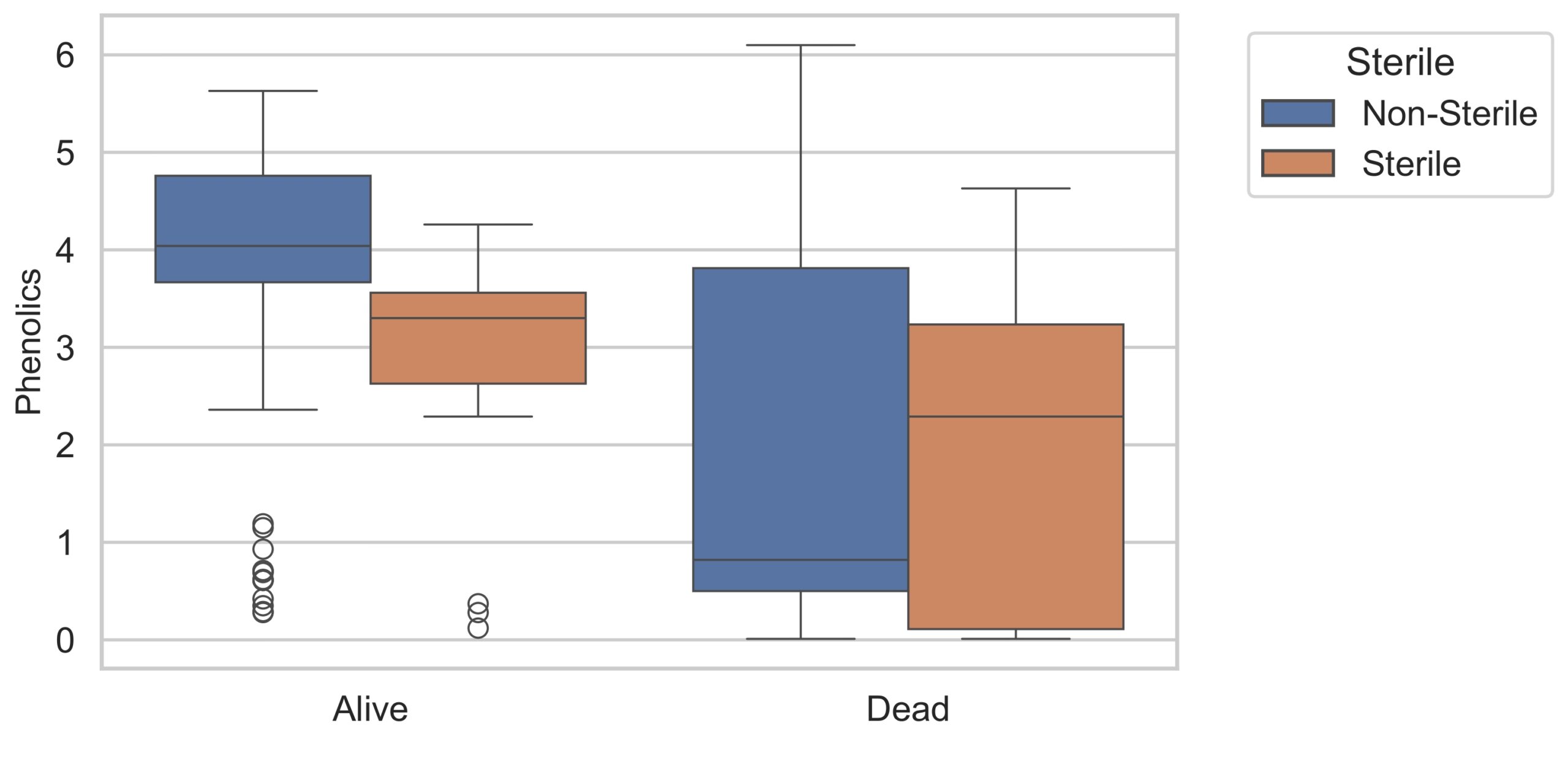
Figure 5 shows the relationship between phenolics and conspecific with respect to target variable Alive. Lowest median and smallest interquartile range out of all three types of conspecific is observed in sterile for both Dead and Alive seedlings.  

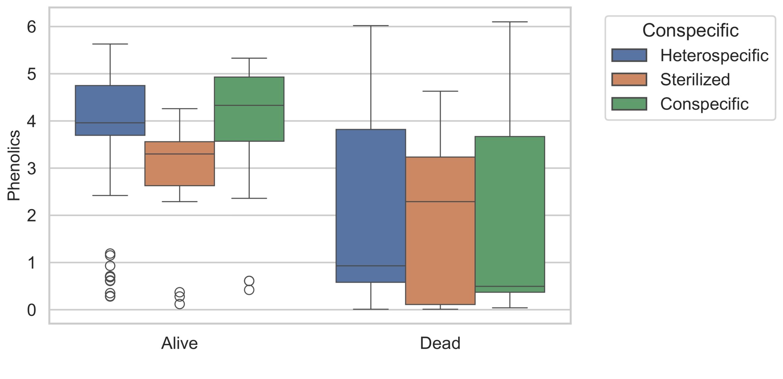
Figure 6 shows the relationship between phenolics and the target variable Alive with respect to soil type. All the Alive seedling’s median phenolics is higher than those of Dead seedlings’ one. In Alive seedlings, the district low phenolics median is observed in Prunus serotina and sterile soil.

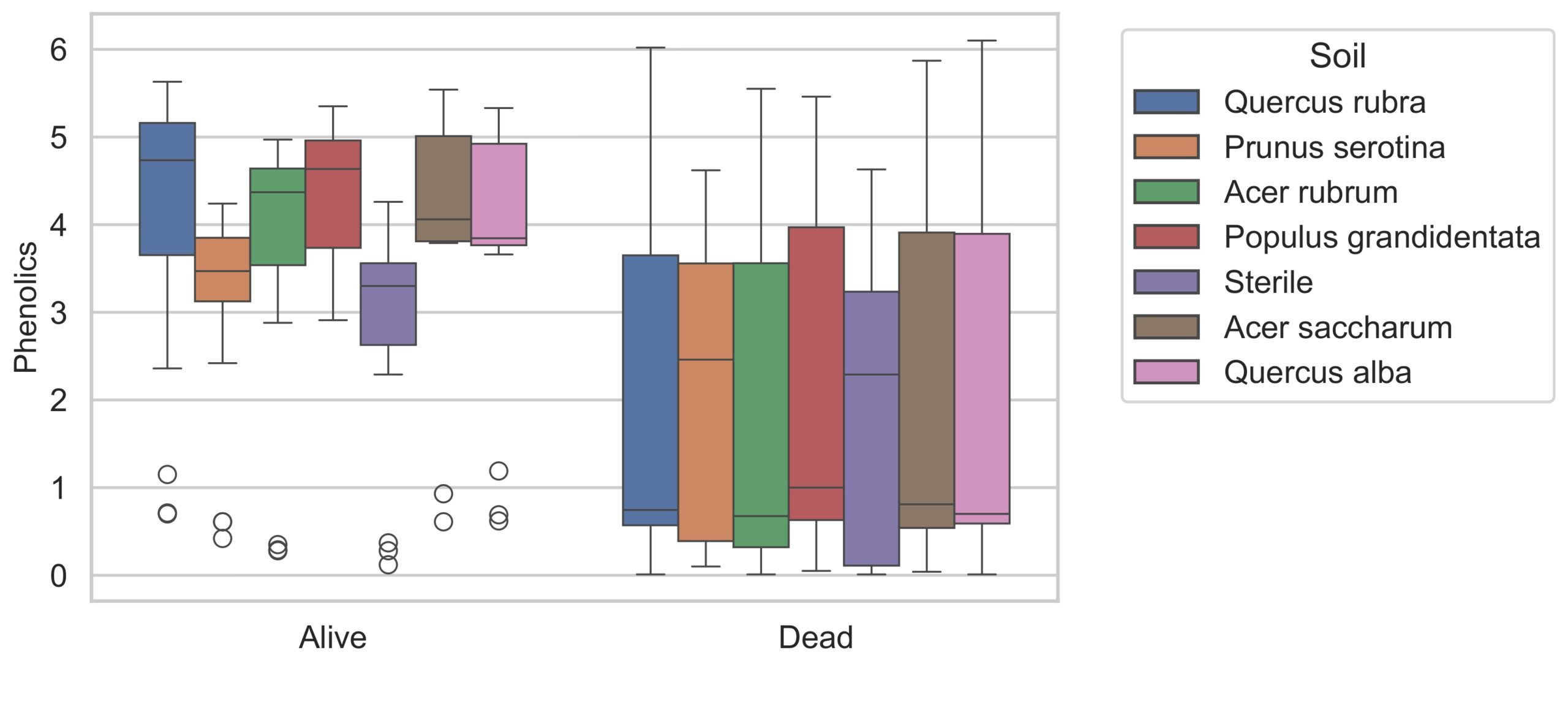
Figure 7 illustrates the relationship between phenolics and target variable Alive with respect to soil myco. Comparing the median of Alive to Dead seedlings, the value is always higher for Alive seedlings. The interquartile range also decreases for Alive seedlings. The lowest median is sterile for both Alive and Dead seedlings while the highest is EMF. 

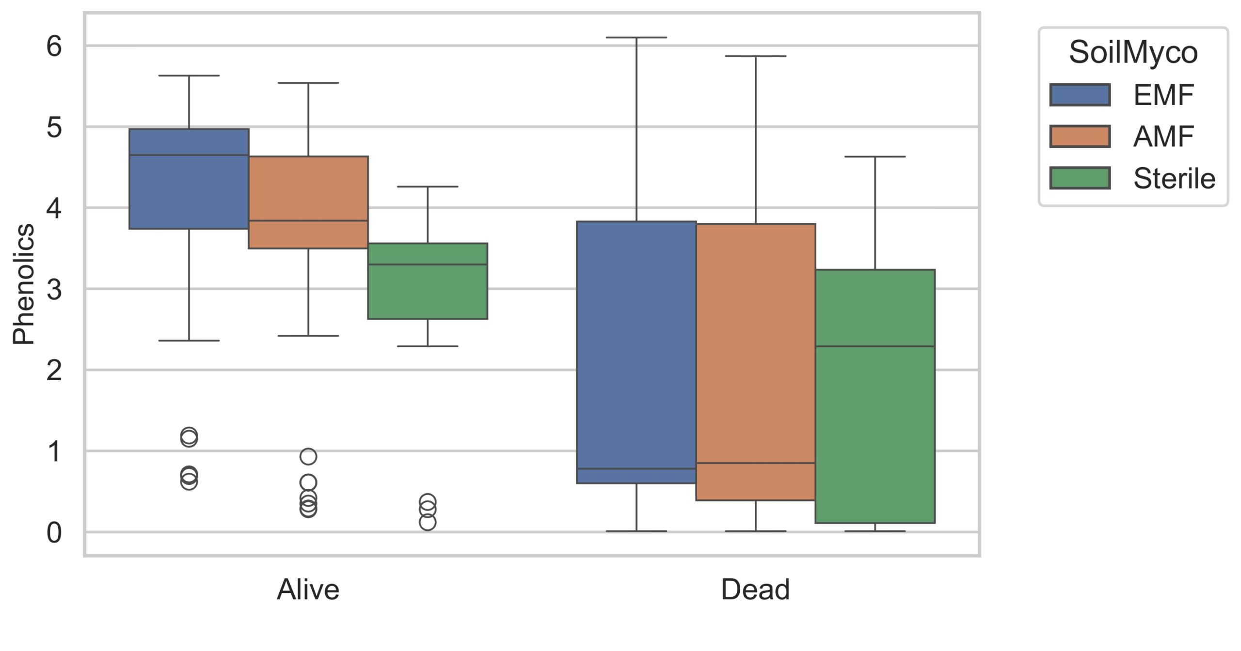
Figure 8 shows the Spearman correlation matrix between numeric variables. The red color indicates positive correlation. On the other hand, the blue indicated a negative relationship. Phenolics, lignin, and NSC are relatively  highly correlated feature pairs. The correlation between NSC and lignin is 0.62, NSC and phenolics is 0.74, and phenolics and lignin is 0.63. Despite the presence of some relatively high correlations in the data set there is no strong evidence of collinearity (||coefficient|| > 0.8).

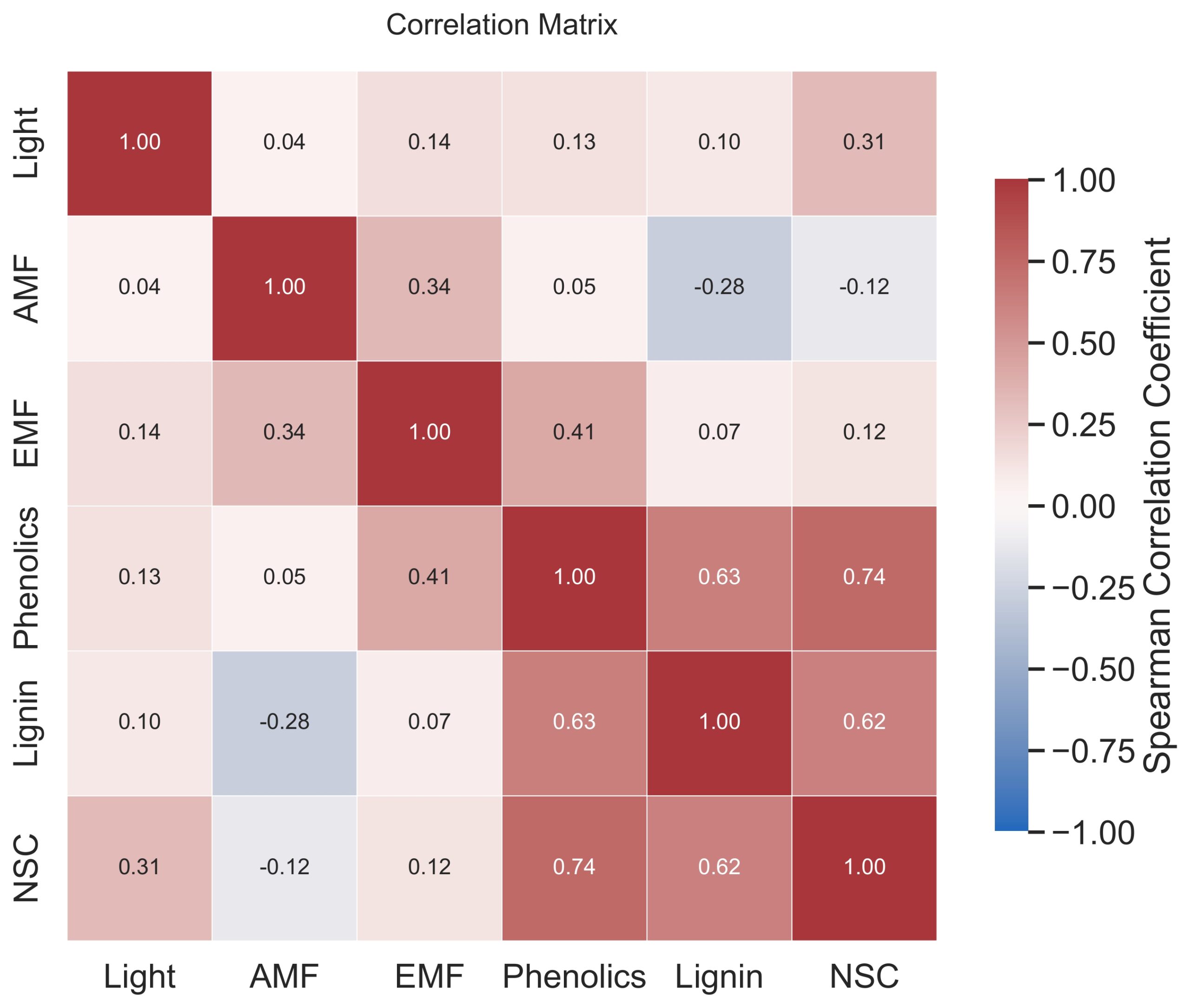
Figure 9 depicts the relationship between phenolics and NSC with respect to species types. There is a positive relation between phenolic and NSC separated by species clusters.  The Acer saccharum cluster has the least amount of NSC and phenolics. Meanwhile, Quercus alba has the most phenolics and NSC values. It appears that Quercus alba and Quercus rubra clusters slightly overlap.  Quercus species clusters are well separated from Prunus and Acer species clusters. 

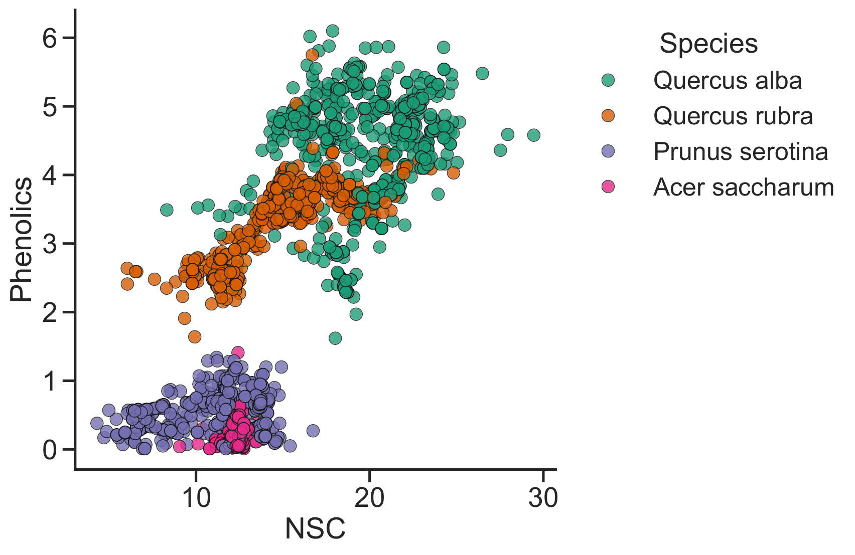
Figure 10 shows the relationship between lignin and phenolics with respect to target variable Alive. Two separate clusters are observed in Dead seedlings but only one of the clusters overlap with Alive seedlings. The bottom cluster includes only myco AMF and mainly Dead samples, and the top cluster includes only myco EMF samples with overlapping Alive and Dead classes.

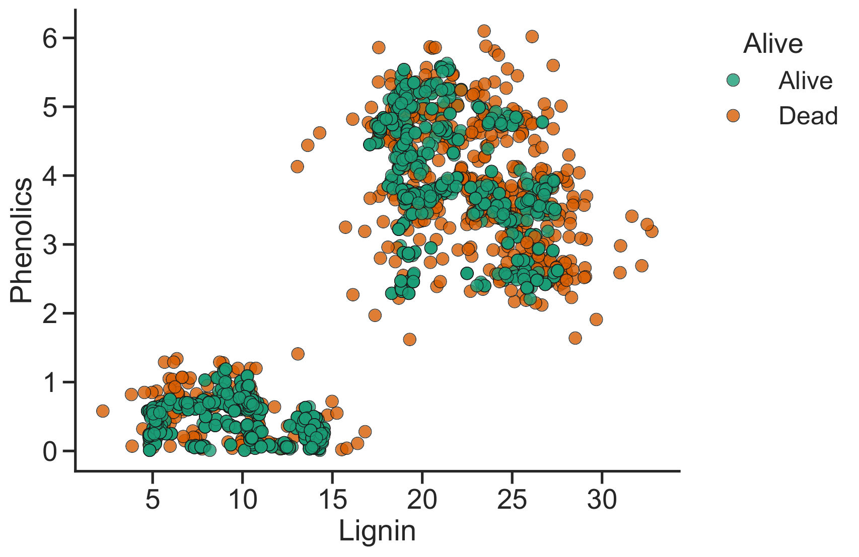
Figure 11 illustrates the relationship of phenolics and lignin with respect to soil type. There are two well separated clusters similarly to Figure 10. It appears that soil type has no effect on phenolics and lignin relationships because of significant overlap in the data.

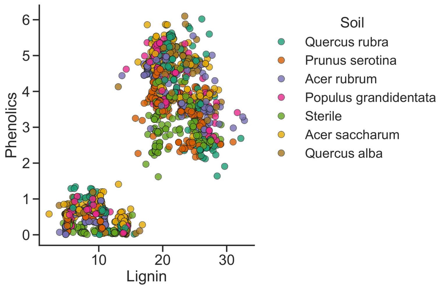
Figure 12 illustrates the relationship between phenolics and lignin with respect to myco EMF and AMF. The separation between AMF and EMF is very apparent. While AMF has high levels of phenolics and lignin, EMF has much lower levels.

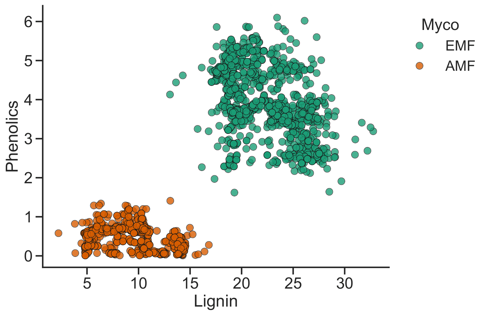
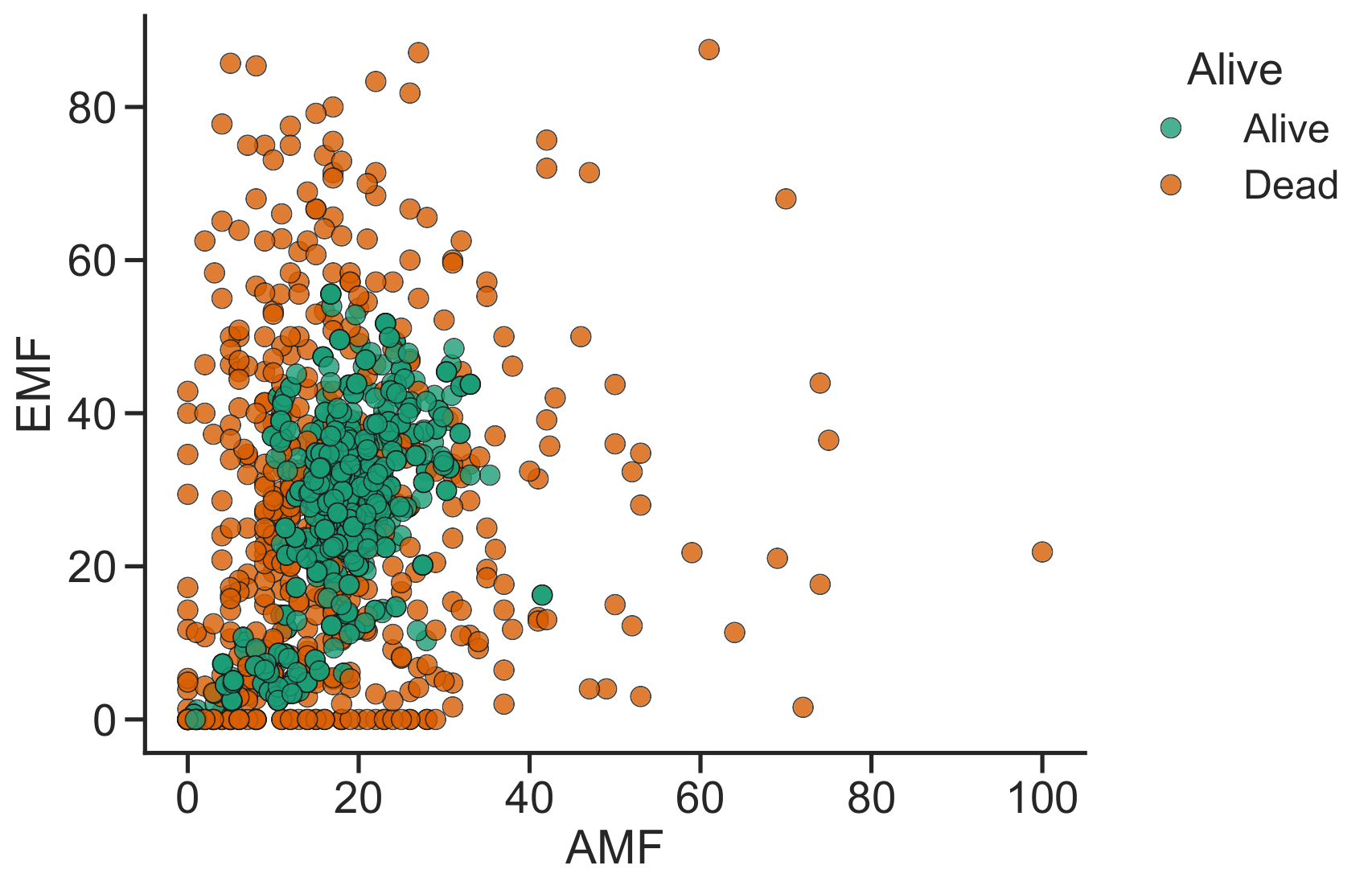
Figure 13 demonstrates the relationship between EMF and AMF colored by the target variable Alive. Data is clustered in the bottom left corner. Most of the Alive seedlings data points are concentrated in the corner while Dead seedlings data points are spread out.

Methodology

Input Features and Output Target

The target output is Alive which indicates if seedling was Alive or Dead at the end of the first growing season. EMF feature is removed due to the significant presence of missing values (~54%). Including EMF would have required significant imputation, which could add unnecessary assumptions and limitations given our dataset. Plant date was removed based on their lack of relevance to the prediction of tree survival. Time variable was excluded because it could potentially introduce data leakage that could directly reveal the outcome of the survival prediction. The remaining input features are species, soil, sterile, conspecific, light, soil myco, myco, AMF, NSC, lignin, and phenolics. 

Data Preprocessing

Encoding Categorical Features

In order to include categorical features into the models, we converted the categorical features into numerical. Categorical features are species, soil, sterile, conspecific, soil myco, and myco as shown in Table 1. Sterile is a binary feature where 0 indicates not sterilized soil and 1 refers to sterilized soil. Species, soil, conspecific, and myco features are encoded using the one hot encoding. One hot encoding is a method for transforming categorical features into numerical columns where each unique category is represented by a binary column with a value of 1 showing its presence and 0 showing its absence. The unique categories of each categorical feature can be found in Table 1. Our target column Alive  is a binary column where 1 indicates seedling was alive at the end of the first growing season and 0 indicates the seedling was dead.

Scaling Numeric Features

We applied feature scaling only for models (e.g. Logistic Regression and KNN), which are sensitive to differences in feature magnitude. We used a StandardScaler to make scale input features by subtracting the mean and dividing by the standard deviation of each feature. The scaler was fitted on the training data and the same transformation was applied to the test data to avoid data leakage. 

Models and Evaluation Metrics

We divided our dataset into training and testing sets using an 80:20 ratio. To ensure that each label category accurately represented the original distribution, we used a stratified split by label³⁷. This method preserves the same ratio of each class in both the training and testing sets. By maintaining this balance, the model can learn effectively from the training data and be fairly evaluated on the test data.

Note that the original experiment is a blocked factorial design, with many seedlings in the same field plot. However, plots do not represent the same environmental units. Across the different plots, soil, species, and light availability vary within plots, and most of this variation occurs at the seedling scale. Holding out entire plots does not cleanly withhold a distinct, consistent set of environmental conditions. Thus, a plot-level train-test split would therefore be expected to yield a training–testing separation similar to the approach we used above.

We trained and tested different machine learning models such as Logistic Regression, K-Nearest Neighbors (KNN), Random Forest, and XGBoost. Logistic Regression finds the best line to separate the Alive and Dead classes. It is a simple model that performs well when there is a clear separation between the classes. The disadvantages include sensitivity to outliers and poor performance when the data has complex and nonlinear relations³⁸. K-Nearest Neighbors (KNN), categorizes the point based on the neighbor points around it. It is simple to understand, and works well in linear and non-linear data. It is also slow and sensitive to outliers³⁹. 

Random Forest creates multiple decision trees, each trained on a random subset of data and features, and then combines their results. It is a powerful model that can handle large datasets, and has less overfitting compared to a single decision tree. But it is also slow, not interpretable, and can be prone to overfitting if not tuned properly ⁴⁰. XGBoost creates decision trees sequentially and for every new tree it finds and corrects the mistakes of the last one. It can handle large and complex datasets efficiently. But, it is also more complex with multiple hyperparameters resulting in being challenging to tune and interpret⁴¹.

We evaluated model performance using precision, recall, and F1-score⁴². Precision quantifies the proportion of predicted positives that are truly positive, recall measures the proportion of actual positives the model correctly identifies. F1 score is  the harmonic mean of precision and recall. In addition, we computed ROC AUC, which aggregates performance across classification thresholds by tracking the true–false positive trade-off, and precision-recall, PR AUC, which summarizes the precision–recall trade-off and is especially informative under class imbalance⁴³. We compare these metrics on the training and test sets to assess overall performance and identify potential overfitting.

Hyperparameter Tuning

Hyperparameter tuning is used to select the combination of model parameters that lets a model learn most effectively. We used grid search to explore parameters values as shown in Table 2. The goal is to identify the parameter combination that maximized performance of the model⁴⁴. To evaluate each parameter combination and quantify the variability, we ran repeated (10 times) stratified 3-fold cross-validation, which preserves the Alive/Dead class balance in every split and lets us compute confidence intervals for all evaluation metrics.

We used Logistic Regression as a baseline linear classifier. This is done to provide a clear reference point (linear decision boundary with well-understood behavior) against any gains from non-linear models (Random Forest, XGBoost). For the k-Nearest Neighbors model (Table 2), we tuned hyperparameters that directly control neighborhood size, similarity definition, and how strongly nearby samples influence predictions. We varied n_neighbors across a range from 1 to 50 values to balance the classic bias–variance trade-off: low k captures local structure but can overfit noise, while higher k smooths the decision boundary and can underfit. We compared weights of {“uniform”, “distance”} to test equal voting against distance-weighted voting, where closer neighbors receive more influence—often improving robustness when neighbors vary in proximity. We also tuned the distance metric, using Minkowski. Because KNN is distance-based and sensitive to feature scale, we scaled all features using Standard Scaler.

For the Random Forest (Table 2), we tuned each hyperparameter with empirical and literature-based evidence. We compared bootstrap {True, False} to test classical bagging—sampling with replacement to decorrelate trees and reduce variance—against using the full dataset per tree. We set class_weight {“balanced”, “balanced_subsample”} to counter Alive/Dead class imbalance, which is defined as weighting classes inversely to their frequencies. We varied max_features between  1 and 25 (up to the full encoded feature set) with increment of 1 to manage the bias–variance trade-off by controlling inter-tree correlation: smaller feature subsets decorrelate trees; larger ones strengthen individual trees. To control growth of the tree we increased min_samples_split between 20 and 100 with an increment of 5, since larger thresholds restrict fine splits and help curb overfitting. We tried n_estimators {100,200,500,1000} because adding trees typically lowers variance with diminishing returns, so performance plateaus after a few hundred to ~1000 trees. 

For the XGBoost model (Table 2), we varied colsample_bytree from 0.5 to 1.0 with increment of 0.1 to apply column subsampling at the tree level. We also varied the subsample from 0.5 to 1.0 with increment of 0.1 to inject row subsampling each boosting round, which helps prevent overfitting. We tested learning_rate between 0.001 and 0.03 to control shrinkage strength. It reduces each step to make boosting more conservative, and the original paper highlights shrinkage as a core overfitting guard. We paired those rates with n_estimators  {100, 200, 500, 1000} to test the standard trade-off that lower learning rates typically require more trees (diminishing returns after a few hundred is common). Finally, we tuned scale_pos_weight broadly (0.01–100) to handle class imbalance, leveraging the library’s guidance that it rebalances positive vs. negative instances.

Model	Parameter	Range
KNN	n_neighbors	Between 1 and 50 with an increment of 1
	weights	“uniform” and “distance”
	metric	minkowski, cosine
Random Forest	n_estimators	{100, 200, 500, 1000}
	max_features	Between 1 and 25 with an increment of 1
	min_samples_split	Between 20 and 100 with an increment of 5
	class_weight	balanced, balanced_subsample
	bootstrap	{True, False}
XGBoost	colsample_bytree	Between 0.5 and 1.0 with increments of 0.1
	learning_rate	{0.001, 0.002, 0.003, 0.01, 0.02, 0.03, 0.1, 0.2, 0.3}
	n_estimators	{100, 200, 500, 1000}
	scale_pos_weight	{0.01, 0.1, 0.5, 1, 5, 10, 20, 30, 40, 50, 100}
	subsample	Between 0.5 and 1.0 with increments of 0.1

To evaluate training performance, we used repeated (10 times) stratified 3-fold cross-validation and calculated the mean ± 95% confidence interval (CI) of all metrics across all folds and repeats. We saved the evaluation metrics separately for the Alive and Dead classes from every repeated split, averaged them to get the cross-validated mean, and computed its 95% confidence interval. 

To evaluate the test performance, we calculated 95% confidence intervals using a bootstrap with 1,000 resamples of the test predictions⁴⁵. For each bootstrapped resample, we computed all evaluation metrics for the Alive and Dead classes. We then calculated the bootstrap mean with its 95% confidence interval.

Our hyperparameter tuning included a broad search range (for both Random Forest and XGBoost) combined with 10x repeated 3-fold cross-validation. Repeated CV helps reduce variance in performance estimates. However, an exhaustive search over many hyperparameter combinations can still increase the chance of selecting configurations that perform well on CV partly due to randomness. Therefore, we acknowledge a potential optimism risk in CV-based model selection without  nested CV. We report final performance on an independent held-out test set that was not used during tuning. Future work could further reduce selection bias by using nested CV or a dedicated validation set.

Paired Model Comparison with McNemar’s Test

After tuning, we compared models on the same test set using statistical significance McNemar’s test⁴⁶ to understand if the difference between the model’s accuracy is luckily due to chance.  This paired test isolates the cases where the models disagree, when one prediction is correct and the other is not, then checks if those discordant counts are symmetric. The output p-value tests the null hypothesis of equal error rates. p-value<0.05 indicates the observed difference between models’ performances is unlikely due to chance. Therefore, one model outperforms the other on the identical examples. 

Handling Data Imbalance

In our dataset, there is a moderate class imbalance between Alive and Dead tree seedlings. The count of Dead tree seedlings (2292) is greater than the Alive ones (491). This imbalance may introduce bias into the model, as a result favoring Dead class predictions. To address the class imbalance issue, we explored different mitigation strategies and compared model performance across them. As it was mentioned above, the data were split into training and test sets using a stratified 80/20 split. All imbalance handling approaches were applied only to the training data, while the test set was kept unmodified to ensure a fair and consistent comparison of methods under the same evaluation conditions. Thus, the original training set class counts were 393 Alive and 1833 Dead (stratified 80/20 split).

The first approach we used was a case of cost-sensitivity learning, such as class weighting during the model training.  We used algorithm-specific weighting during training⁴⁷. For Random Forest, we used the built-in class_weight=”balanced” or “balanced_subsample” parameter, which weights classes inversely to their frequencies. It up-weights the minority (e.g., Alive) class and down-weights the majority (Dead) class. For XGBoost, we varied the scale_pos_weight parameter to reflect the class imbalance ratio, increasing the contribution of the minority (e.g., Alive) class to the loss and gradients.

Another approach we used was undersampling⁴⁸. This method removes a random subset of the majority class in the training data to match the size of the minority class. The model takes an equal number of samples from both Alive and Dead classes during training.  But the disadvantage is that we remove potentially useful observations. As noted above, the test set was not modified and remained sampled from the original data distribution for all evaluations. After undersampling, the training set was balanced to 393 Alive and 393 Dead samples.

Lastly, we explored the oversampling technique by expanding the minority (Alive) class in the training data to approximate the majority (Dead) class size. We applied SMOTE (Synthetic Minority Over-Sampling Technique), which generates synthetic Alive samples by interpolating between existing minority instances (Chawla et al., 2002). We also used ADASYN, an adaptive variant that focuses synthesis on harder-to-learn minority examples⁴⁹. Oversampling was applied only to the training dataset, while the test set was kept unmodified and retained its original class distribution. Within cross-validation, oversampling was applied independently within each CV split, applying SMOTE/ADASYN only to the CV training fold (after the fold split) and leaving the corresponding validation fold unchanged, thereby preventing any synthetic-sample leakage between folds. After oversampling, the training set class counts were approximately balanced at 1833 Alive (synthetic + original) and 1833 Dead.

Feature Importance Analysis

Feature importance analysis is a technique that is used to evaluate which input variables have the strongest or weakest influence on a model’s predictions. SHAP is a method used to explain how machine learning models make their predictions⁵⁰. This helps with understanding which features are most important and how much each one contributed to a specific prediction. SHAP calculates how much each feature contributes to a machine learning model’s prediction. With these calculations, the inputs can be shown if it gives a positive or negative effect and by how much. We implemented SHAP analysis to understand and quantify the contribution of tree seedling and soil characteristics, light information, fungal colonization, and biochemical characteristics, on model predictions of Alive or Dead seedlings.

Results and Discussion

Results from Cost-Sensitive Learning – Class Weighting Approach

Evaluation metrics and hyperparameter settings were assessed for models trained on the original training dataset using a class weighting approach to address class imbalance. The comparison focused on key performance indicators—F1 scores, ROC AUC, and PR AUC across cross-validation (CV) and test sets, along with their corresponding confidence intervals to evaluate performance stability and generalization across models. The detailed evaluation metrics with corresponding confidence intervals and optimal hyperparameter settings for each model are reported in Appendix, Table A1. Overall, the results show that Logistic Regression, KNN, and XGBoost achieved nearly identical F1 performance on the minority class, while Random Forest provided the best and most stable balance across all metrics. Its higher test F1, ROC AUC, and PR AUC scores demonstrate superior generalization and robustness under the class-weighted training approach.

Across models, the F1 scores for the Alive class on the test set were fairly similar for Logistic Regression, KNN, XGBoost, while Random Forest achieved a clear improvement. Logistic Regression recorded an Alive test F1 of 52.3% ±6.4%, KNN scored 53.5% ±8.4%, and XGBoost achieved 52.1% ±8.8%—all within a close range as shown in Figure 14 (top). The Dead class showed consistently strong performance across these models, with test F1 values of 78.1% ±3.4% for Logistic Regression, 89.3% ±2.1% for KNN, and 90.1% ±2.0% for XGBoost. The Random Forest model notably outperformed the others for the Alive label, reaching a test F1 score of 62.3% ±6.6%, while maintaining a competitive Dead class test F1 score of 87.0% ±2.3%.

All models demonstrated strong overall test ROC AUC values in the mid-to-high 80% range as shown in Figure 14 (bottom). Logistic Regression achieved Alive class test ROC AUC score of 84.0% ±3.6%, KNN showed 84.5% ±4.1%, XGBoost reached 86.1% ±3.9%, and Random Forest obtained the highest test ROC AUC score at 88.3% ±3.4%. The narrow confidence intervals across models (±3–4%) indicate stable classification performance across test folds. The ROC curves shown on the left subplot of Figure 15 visually confirm these results—each curve lies well above the diagonal reference line, reflecting effective class discrimination, with the Random Forest and XGBoost curves exhibiting the largest area under the curve. However, it is important to note that ROC AUC may not be a fully reliable indicator for imbalanced data, as it assigns equal weight to both classes. Therefore, while all models showed strong separation ability, evaluating PR AUC provides more insight into their true performance on the minority Alive class.

The PR AUC test scores reveal greater differences between models and better reflect the challenges of imbalanced data as shown in Figure 14 (bottom). Logistic Regression had the lowest Alive class test PR AUC at 43.1% ±9.0%, indicating limited precision when identifying minority cases. KNN improved modestly to 47.7% ±9.2%, and XGBoost performed slightly better with 51.8% ±10.1%, but all three exhibited wide confidence intervals, suggesting instability in minority-class predictions. The Random Forest model again led with the highest Alive test PR AUC of 55.6% ±10.3%. These results show that while all models struggled to achieve high PR AUCs for the minority class, Random Forest maintained the most reliable performance under class imbalance among the models. The right subplot in Figure 15 showing the PR curves highlights these trends—Random Forest and XGBoost maintain the highest precision across most recall values, while Logistic Regression’s curve drops steeply, emphasizing its lower precision at high recall. These visual results complement the quantitative metrics, confirming that Random Forest and XGBoost achieved the most robust performance on the minority Alive class. 

When comparing train and test performance, all models demonstrated limited overfitting and maintained consistency between CV train and test sets as shown in Table A1. Logistic Regression’s F1 and AUC values changed minimally between CV train and test. KNN exhibited similarly stable behavior. XGBoost showed slightly higher variability but maintained solid generalization. Random Forest, despite a marginal decrease in PR AUC, preserved strong and stable F1, ROC and PR AUC scores. Confidence intervals generally widened from train to test across all models, particularly for F1 and PR AUC in the Alive class as shown in Table A1. F1 score confidence interval for the Alive class increases from ±2–5% in CV train to ±6-9% in test, and PR AUC score confidence interval increases from ±4-6% in CV train to ±9-11%. This reflects higher variability and uncertainty when models were exposed to unseen minority-class data. The Dead class intervals remained narrower confirming stable majority-class predictions. 

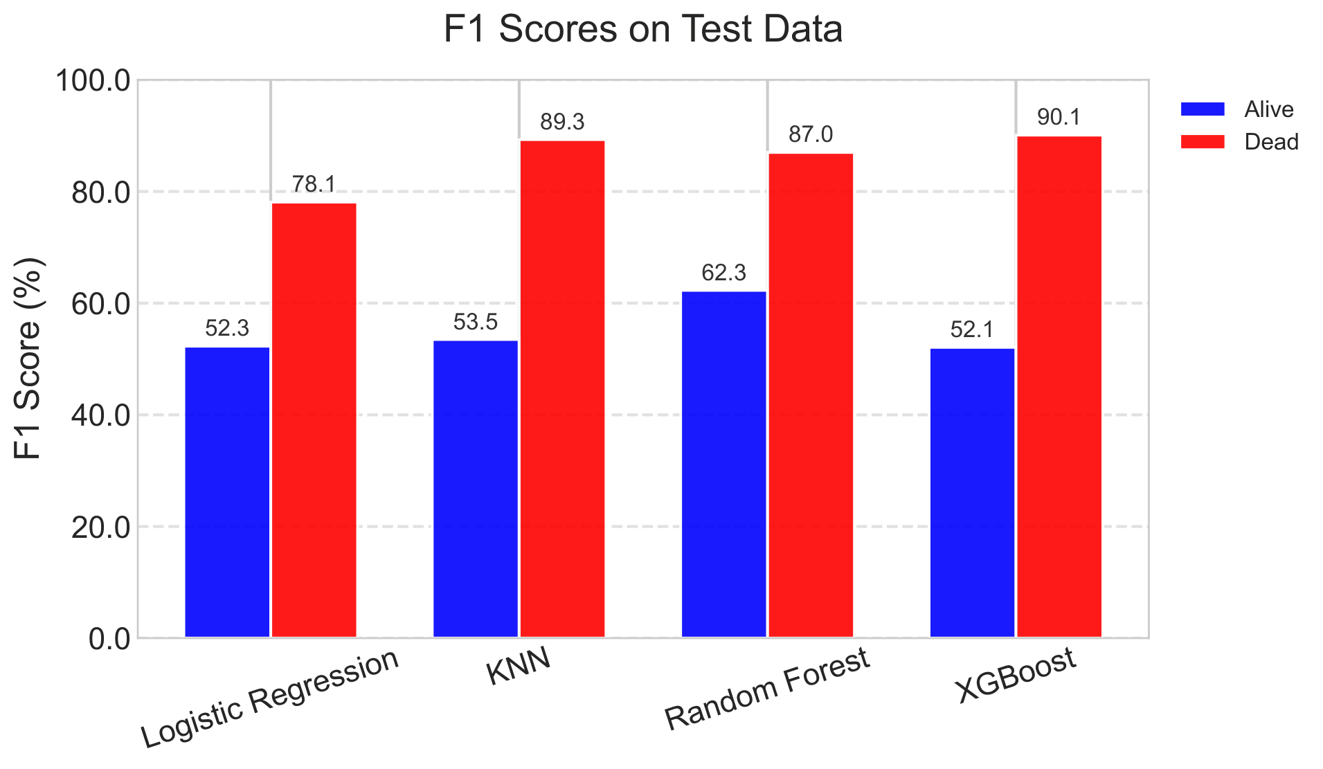
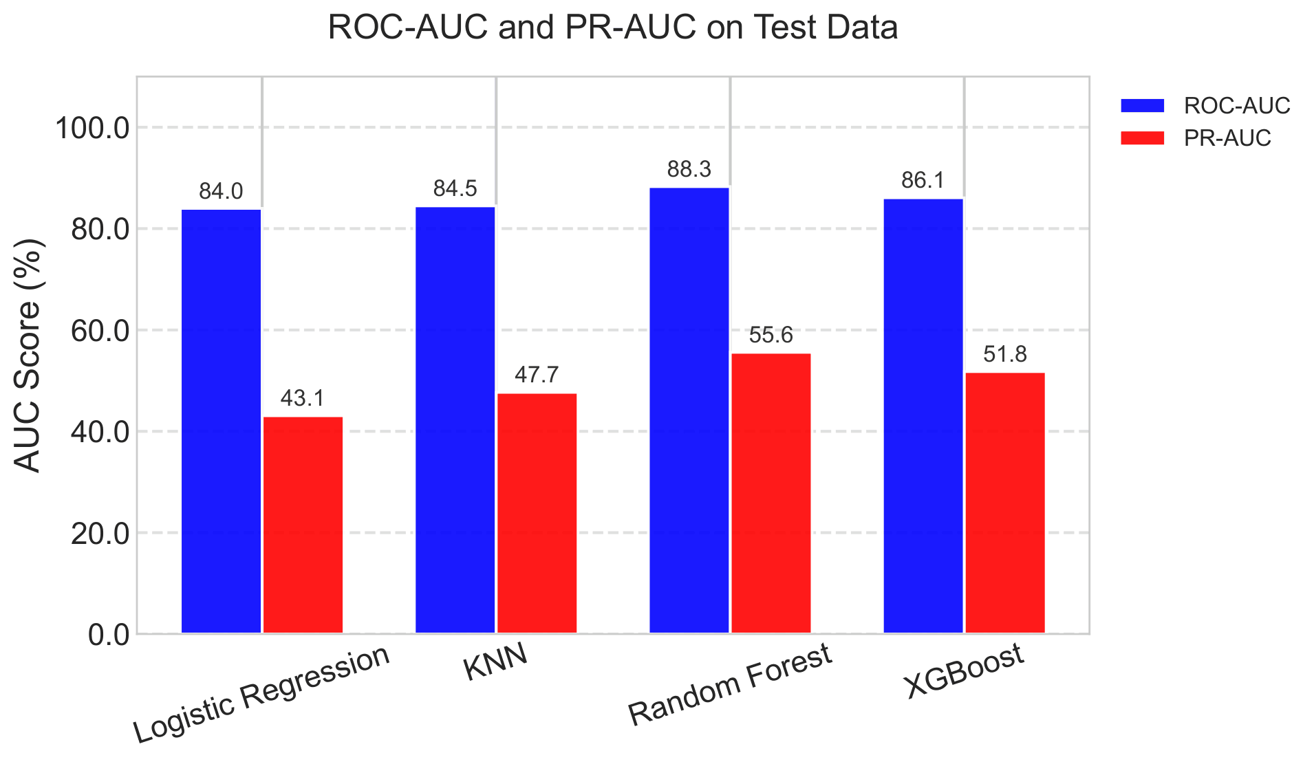
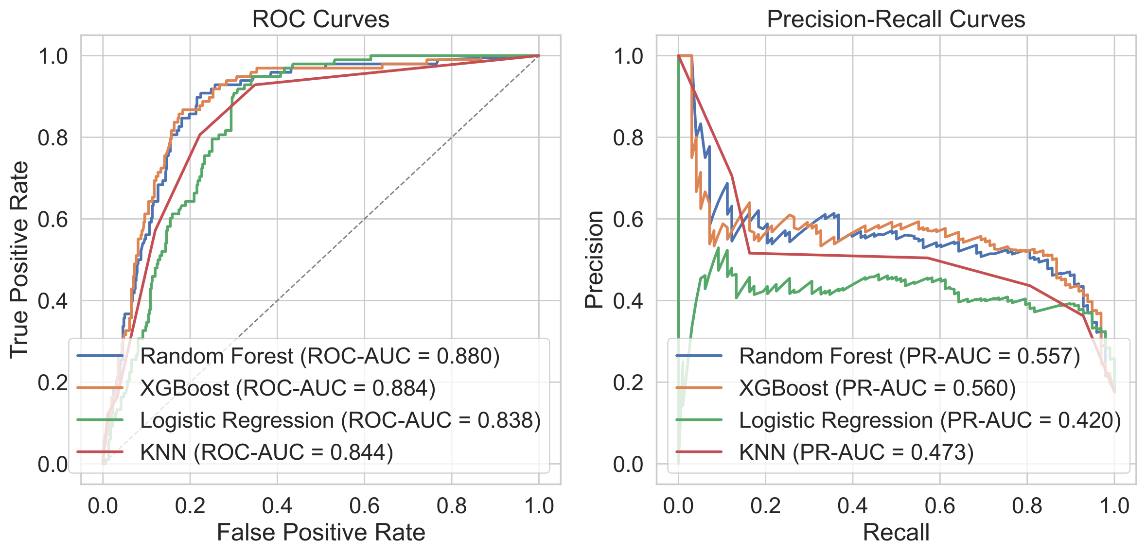
Table 3 presents pairwise McNemar p-values comparing the accuracy of the optimal models on the test dataset, with all models trained on the original training data using a class weighting approach. These p-values test whether the difference in predictive accuracy between two models is statistically significant, with values below 0.05 indicating evidence of a meaningful difference. Overall, the results show that Logistic Regression performs significantly worse than the other models, while XGBoost and Random Forest generally demonstrate the strongest performance.

Logistic Regression differs significantly from all competing models. In the comparison with Random Forest, the p-value is 0.0000, with Random Forest being correct in 66 cases where Logistic Regression is wrong, compared with only 9 cases in the opposite direction. XGBoost also significantly outperforms Logistic Regression (p = 0.0000), with 124 cases favoring XGBoost and 38 favoring Logistic Regression. Likewise, KNN performs significantly better than Logistic Regression (p = 0.0000), with 106 cases where KNN is correct and Logistic Regression is wrong, compared with 36 cases in the reverse direction. These findings consistently indicate that Logistic Regression has the weakest predictive accuracy among the models evaluated.

Among the remaining models, Random Forest and XGBoost differ significantly (p = 0.0030), with Random Forest being correct in 59 cases where XGBoost is wrong, compared with 30 cases favoring XGBoost, indicating that Random Forest achieves significantly higher accuracy. The comparison between XGBoost and KNN is also statistically significant (p = 0.0489), although the evidence is weaker, with 37 cases favoring XGBoost and 21 favoring KNN. In contrast, the comparison between KNN and Random Forest is not statistically significant (p = 0.2034), despite KNN being correct in 51 cases versus 38 for Random Forest. Taken together, these results suggest that Random Forest is the strongest-performing model, Logistic Regression is the weakest, and KNN and XGBoost show comparable performance on the test set.

Model A	Model B	p-value	Model A is correct, Model B is wrong	Model A is wrong, Model B is correct
Random Forest	Logistic Regression	0.0000	66	9
Random Forest	XGBoost	0.0030	59	30
XGBoost	Logistic Regression	0.0000	124	38
Logistic Regression	KNN	0.0000	36	106
KNN	Random Forest	0.2034	51	38
XGBoost	KNN	0.0489	37	21

Results from Undersampled Approach

Evaluation metrics and hyperparameter settings were obtained for models trained on the undersampled training dataset, using optimal parameters selected through cross-validation. The comparison focuses on F1 scores, ROC AUC, and PR AUC, with accompanying confidence intervals (±) to assess stability and generalization across models. The detailed evaluation metrics with corresponding confidence intervals and optimal hyperparameter settings for each model are reported in Appendix, Table A2.

Across the models, the Alive class test F1 scores were moderate and generally comparable across KNN and XGBoost, while Logistic Regression performed slightly lower and Random Forest achieved the strongest minority-class performance as shown in Figure 16 (top). Logistic Regression achieved an Alive test F1 score of 52.5% ±6.5%, KNN improved this to 55.1% ±6.7%, and XGBoost reached 55.0% ±6.6% as shown in Table A2. Random Forest produced the highest Alive test F1 score at 59.8% ±6.4%, indicating the best overall precision–recall balance for the minority Alive class under undersampling approach. For the Dead class, Logistic Regression reached a test F1 score of 78.5% ±3.1%, KNN improved to 82.4% ±2.9%, XGBoost achieved 83.3% ±2.9%, and Random Forest again led with 85.4% ±2.6% (Table A2). Overall, the undersampling approach enabled all models to achieve moderate test performance on both classes, with Random Forest and XGBoost demonstrating the strongest F1 performance.

All models exhibited strong discriminative ability based on ROC AUC, with values consistently in the mid-80% range on the test set as shown in Figure 16 (bottom). Logistic Regression achieved a test ROC AUC of 84.1% ±3.5%, KNN was similar at 84.3% ±3.6%, and XGBoost improved to 85.9% ±4.0% as shown in Table A2. Random Forest achieved the highest test ROC AUC at 86.7% ±3.6%, reflecting the strongest overall class separation among the models. The relatively narrow confidence intervals (±3–4%) indicate stable discrimination across test folds. Taken together, the ROC AUC results align with the test F1, with Random Forest and XGBoost showing the most consistent overall discrimination. The ROC curves shown on the left subplot of Figure 17 visually confirm these results—each curve lies well above the diagonal reference line, reflecting effective class discrimination, with the Random Forest and XGBoost curves exhibiting the largest area under the curve. 

The test PR AUC values further highlight differences in minority-class precision–recall performance under undersampling approach as shown in Figure 16 (bottom). Logistic Regression achieved an Alive PR AUC of 44.7% ±8.9%, KNN was similar at 43.7% ±7.8%, while Random Forest improved to 51.7% ±10.0% as shown in Table A2. XGBoost delivered the highest Alive PR AUC at 52.2% ±10.3%, indicating the most favorable precision–recall trade-off for the Alive class and the strongest ability to control false positives. Confidence intervals for PR AUC were wider than those for ROC AUC ( ±8–10%), reflecting greater variability in precision across folds. Overall, the PR AUC results reinforce that Random Forest and XGBoost provide the most robust minority-class performance under undersampling, consistent with their stronger test F1 and ROC AUC values. The right subplot in Figure 17 showing the PR curves highlights that Random Forest and XGBoost maintain the highest precision across most recall values, while Logistic Regression’s curve drops steeply, emphasizing its lower precision at high recall. These visual results complement the quantitative metrics, confirming that Random Forest and XGBoost achieved the most robust performance on the minority Alive class. 

Across all models, CV train and test performance remained reasonably consistent, suggesting some overfitting despite the reduced training set size inherent to undersampling (Table A2). In general, confidence intervals widened from CV train to test, particularly for the Alive class metrics. For example, Alive F1 confidence intervals increased from approximately ±2–4% in CV train to ±6–7% on the test set , and Alive PR AUC intervals increased from roughly ±4–8% in CV train to ±8–10% in test. Overall, the undersampling approach produced  stable discrimination across models, with Random Forest and XGBoost consistently achieving the highest and most reliable test F1, ROC AUC, and PR AUC performance.

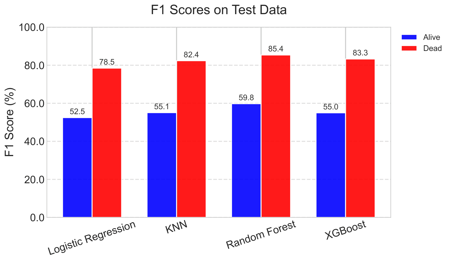
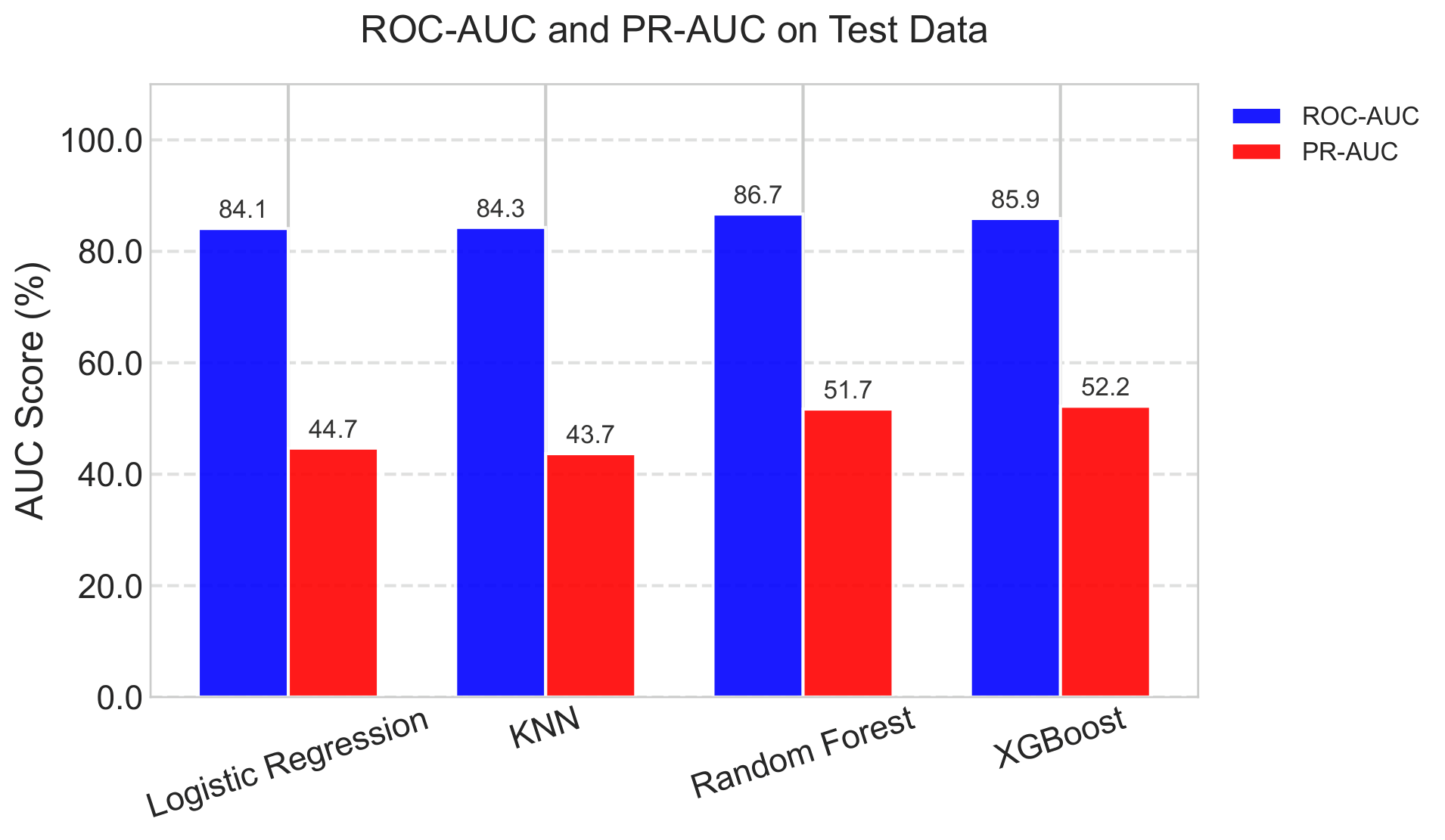
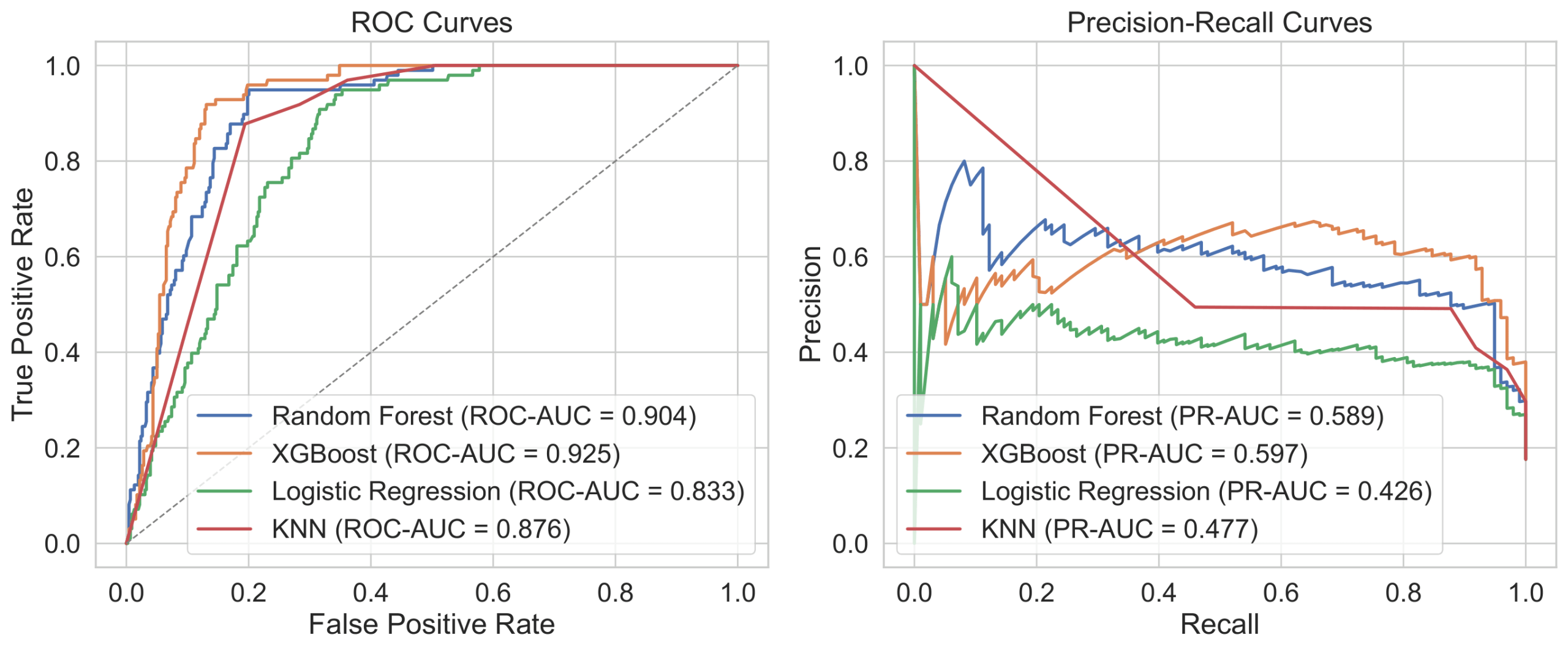
Table 4 presents pairwise McNemar p-values comparing the accuracy of the models on the test dataset when trained on the undersampled training data. These p-values assess whether the difference in predictive accuracy between two models is statistically significant, with values below 0.05 indicating evidence of a meaningful difference. Overall, the results show that Logistic Regression again performs worse than the other models, while Random Forest and XGBoost remain among the strongest-performing approaches.

Logistic Regression differs significantly from all competing models. In the comparison with Random Forest, the p-value is 0.0000, with Random Forest being correct in 53 cases where Logistic Regression is wrong, compared with only 8 cases in the opposite direction. XGBoost also significantly outperforms Logistic Regression (p = 0.0000), with 64 cases favoring XGBoost and 23 favoring Logistic Regression. Similarly, KNN performs significantly better than Logistic Regression (p = 0.0042), with 41 cases where KNN is correct and Logistic Regression is wrong, compared with 18 cases in the reverse direction. These results indicate that Logistic Regression has the weakest predictive accuracy among the undersampling-based models.

Among the remaining models, the comparison between Random Forest and XGBoost yields a p-value of 0.6650, indicating no statistically significant difference in accuracy between them. Random Forest is correct in 26 cases where XGBoost is wrong, while XGBoost is correct in 22 cases where Random Forest is wrong, suggesting that their predictive performance is broadly comparable. In contrast, KNN performs significantly worse than both Random Forest and XGBoost. The comparison between KNN and Random Forest is statistically significant (p = 0.0024), with Random Forest being correct in 35 cases compared with 13 for KNN. Likewise, XGBoost significantly outperforms KNN (p = 0.0184), with 35 cases favoring XGBoost and 17 favoring KNN. Taken together, these findings suggest that under the undersampling approach, Random Forest and XGBoost are the strongest-performing models with comparable accuracy, KNN shows intermediate performance, and Logistic Regression remains the weakest model.

Model A	Model B	p-value	Model A is correct, Model B is wrong	Model A is wrong, Model B is correct
Random Forest	Logistic Regression	0.0000	53	8
Random Forest	XGBoost	0.6650	26	22
XGBoost	Logistic Regression	0.0000	64	23
Logistic Regression	KNN	0.0042	18	41
KNN	Random Forest	0.0024	13	35
XGBoost	KNN	0.0184	35	17

Results from Oversampled Approach

Evaluation metrics and hyperparameter settings were obtained for models trained on the oversampled dataset, using optimal parameters tuned through cross-validation. The comparison highlights F1 scores, ROC AUC, and PR AUC along with confidence intervals (±) to assess the stability and generalization of each model under oversampling. We evaluated two synthetic oversampling methods—SMOTE and ADASYN—and found that both produced very similar performance patterns across all models. Because ADASYN yielded slightly better results overall than SMOTE, we present the ADASYN-based oversampling outcomes in this section. The detailed evaluation metrics with corresponding confidence intervals and optimal hyperparameter settings for each model are reported in Appendix, Table A3. Overall, oversampling yields the strongest and most reliable minority-class performance for the ensemble methods—particularly XGBoost—while Random Forest remains competitive and both outperform Logistic Regression and KNN across most test-set metrics.

Across the models, oversampling produced moderate-to-strong Alive class test F1 scores, with the ensemble methods achieving the most favorable balance and Logistic Regression and KNN performing slightly lower as shown in Figure 18 (top). Logistic Regression achieved an Alive test F1 score of 54.4% ±2.3%, while KNN reached 53.3% ±8.6% as shown in Table A3. Random Forest improved minority-class performance to 59.2% ±6.8%, and XGBoost produced the highest Alive test F1 score at 61.6% ±8.1% (Table A3). For the Dead class, Logistic Regression reached a test F1 score of 79.7% ±1.9%, while KNN achieved 89.2% ±2.1%. Random Forest produced a Dead test F1 score of 87.3% ±2.2%, and XGBoost again led with 90.5% ±2.0% (Table A3). Overall, the oversampling approach improved performance particularly for the minority Alive class, with XGBoost and Random Forest demonstrating the strongest F1 results across both classes.

All models maintained strong discriminative ability based on their test ROC AUC values, with ensemble methods again achieving the highest class separation as shown in Figure 18 (bottom). Logistic Regression achieved a test ROC AUC of 83.4% ±2.5%, while KNN was similar at 84.3% ±3.9% as shown in Table A3. Random Forest achieved the highest test ROC AUC at 87.7% ±3.4%, and XGBoost closely followed at 88.7% ±3.2%, indicating excellent discrimination between Alive and Dead seedlings under oversampling. The ROC AUC confidence intervals remained relatively narrow (approximately ±2–4%), suggesting stable discrimination across evaluation folds, and reinforcing the stronger overall ranking of the ensemble models. The ROC curves shown on the left subplot of Figure 19 visually confirm these results—each curve lies well above the diagonal reference line, reflecting effective class discrimination, with the Random Forest and XGBoost curves exhibiting the largest area under the curve. 

The test PR AUC values further highlight the precision–recall trade-offs for the minority Alive class under oversampling approach as shown in Figure 18 (bottom). Logistic Regression produced a comparatively low Alive PR AUC of 39.8% ±5.2%, while KNN improved to 47.5% ±9.0% (Table A3). Random Forest achieved an Alive PR AUC of 52.8% ±9.9%, and XGBoost produced the highest PR AUC at 54.1% ±9.7%, indicating the most favorable precision–recall balance and strongest ability to limit false positives while capturing Alive seedlings. Confidence intervals for PR AUC (roughly ±5–10%) were wider than those for ROC AUC , reflecting greater variability in precision across folds and models, particularly for KNN and the ensemble methods. The right subplot in Figure 19 showing the PR curves highlights that Random Forest and XGBoost maintain the highest precision across most recall values, while Logistic Regression’s curve drops steeply, emphasizing its lower precision at high recall. These visual results complement the quantitative metrics, confirming that Random Forest and XGBoost achieved the most robust performance on the minority Alive class. 

Across the models, CV train and test performance were generally consistent, indicating limited overfitting despite the expanded training set size introduced by oversampling (Table A3). For example, Random Forest remained close from CV train to test for Alive F1 (62.0% ±4.2% to 59.2% ±6.8%) and ROC AUC (89.5% ±1.7% to 87.7% ±3.4%), while XGBoost showed a similar pattern for Alive F1 (59.1% ±5.0 to 61.6% ±8.1) and ROC AUC (88.7% ±1.7% to 88.7% ±3.2). In contrast, Logistic Regression’s train and test values are identical across all reported metrics (e.g., Alive F1 = 54.4% ±2.3% and ROC AUC = 83.4% ±2.5%), which suggests the same summary values were carried across both splits in Table A3. 

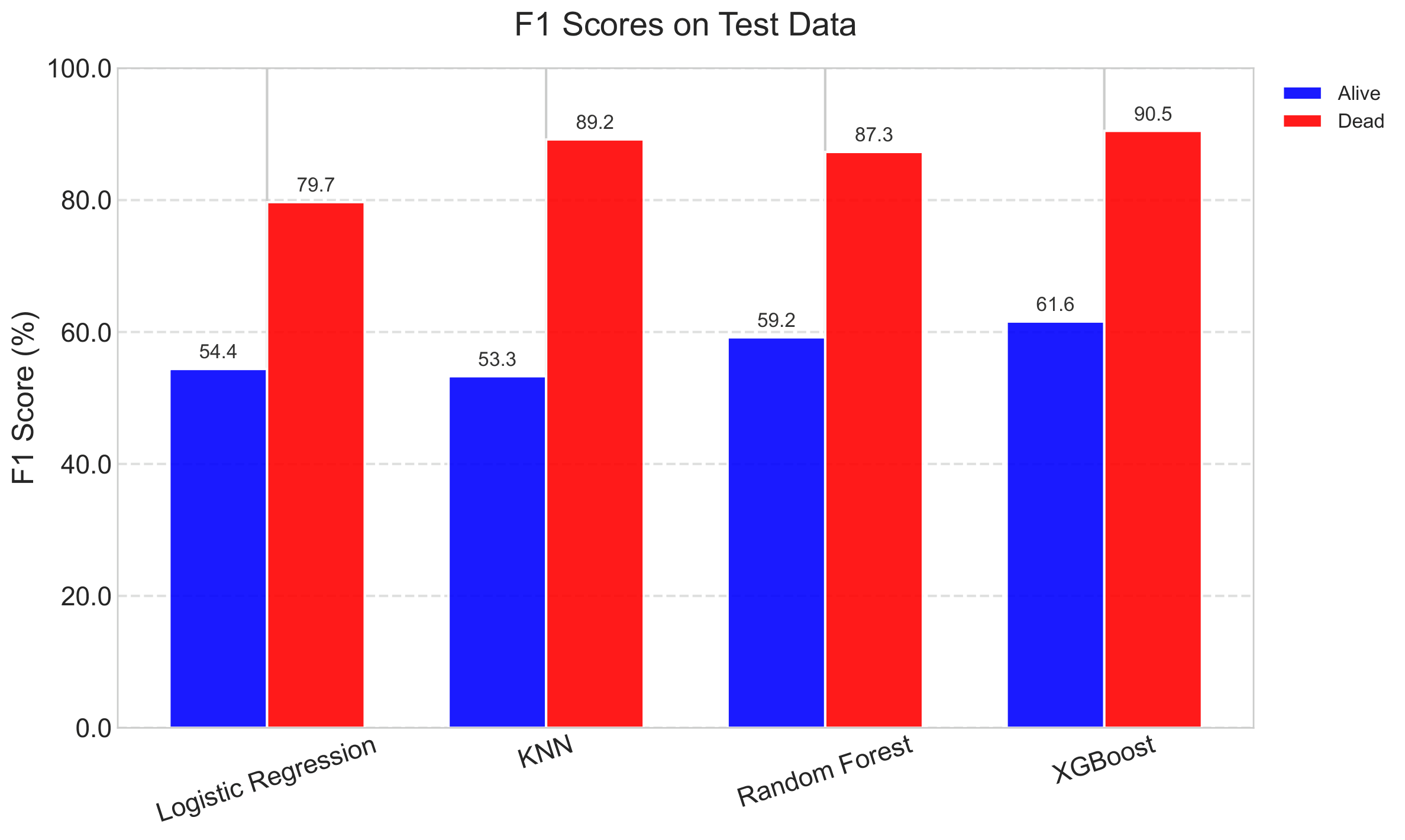
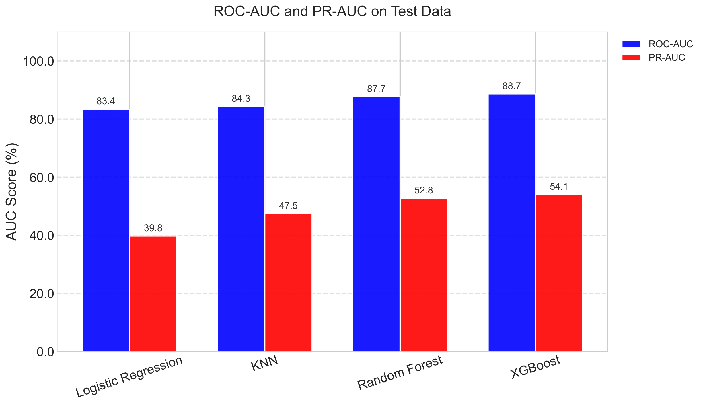
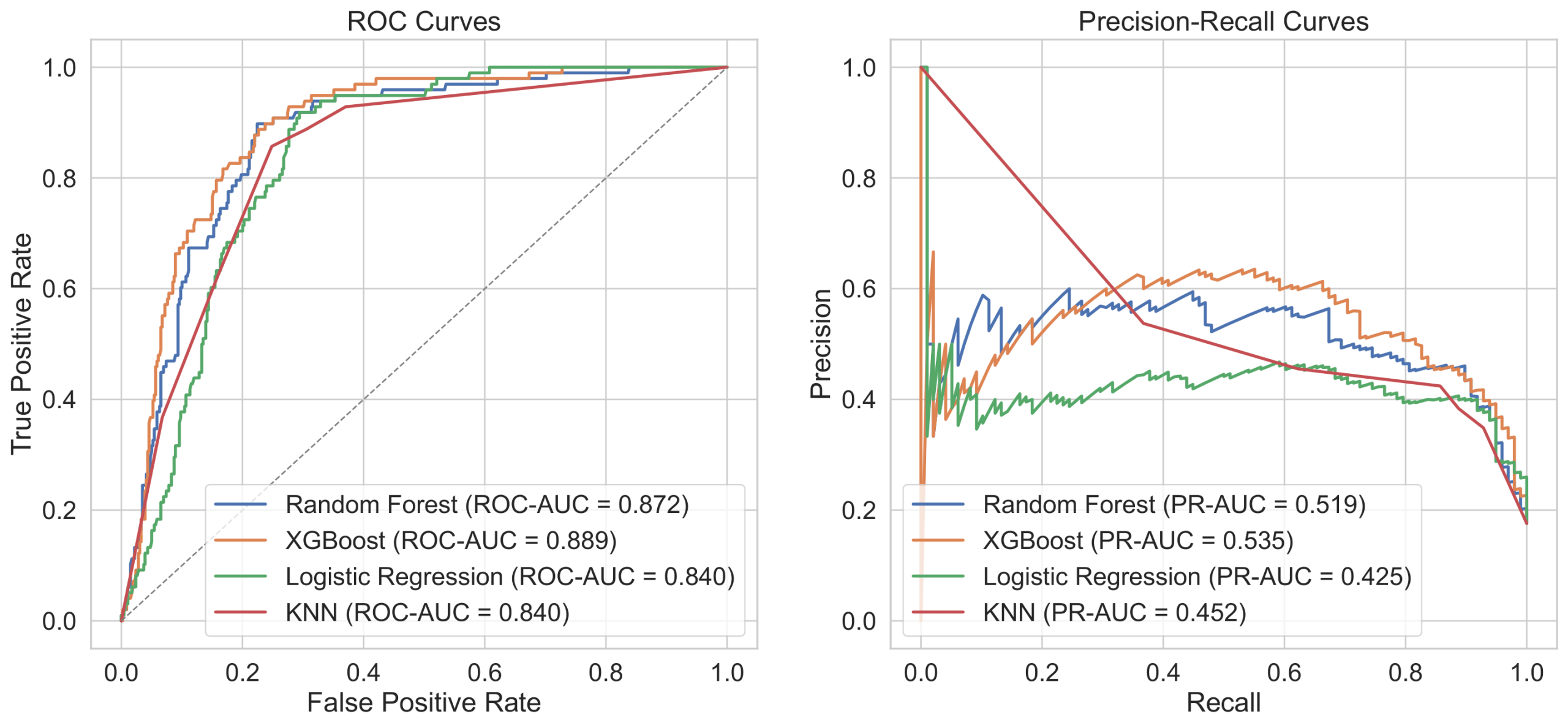
Table 5 presents pairwise McNemar p-values comparing the accuracy of the optimal models on the test dataset when trained on the oversampled training data. These p-values assess whether the difference in predictive accuracy between two models is statistically significant, with values below 0.05 indicating evidence of a meaningful difference. Overall, the results show that Logistic Regression performs significantly worse than the other models, while XGBoost demonstrates the strongest predictive performance.

Logistic Regression differs significantly from all competing models. In the comparison with Random Forest, the p-value is 0.0000, with Random Forest being correct in 76 cases where Logistic Regression is wrong, compared with only 29 cases in the opposite direction. XGBoost also significantly outperforms Logistic Regression (p = 0.0000), with 98 cases favoring XGBoost and 28 favoring Logistic Regression. Likewise, KNN performs significantly better than Logistic Regression (p = 0.0070), with 60 cases where KNN is correct and Logistic Regression is wrong, compared with 33 cases in the reverse direction. These results consistently indicate that Logistic Regression has the weakest predictive accuracy among the models evaluated under the oversampling approach.

Among the remaining models, Random Forest and XGBoost differ significantly (p = 0.0021), with XGBoost being correct in 37 cases where Random Forest is wrong, compared with 14 cases favoring Random Forest, indicating that XGBoost achieves significantly higher accuracy than Random Forest. The comparison between XGBoost and KNN is also statistically significant (p = 0.0000), with 65 cases favoring XGBoost and 22 favoring KNN, showing that XGBoost outperforms KNN by a clear margin. Similarly, the comparison between KNN and Random Forest yields a p-value of 0.0111, with Random Forest being correct in 38 cases where KNN is wrong, compared with 18 cases favoring KNN, indicating that Random Forest also performs significantly better than KNN. Taken together, these findings suggest a clear ranking under the oversampling approach, with XGBoost as the strongest-performing model, followed by Random Forest, then KNN, while Logistic Regression remains the weakest.

Model A	Model B	p-value	Model A is correct, Model B is wrong	Model A is wrong, Model B is correct
Random Forest	Logistic Regression	0.0000	76	29
Random Forest	XGBoost	0.0021	14	37
XGBoost	Logistic Regression	0.0000	98	28
Logistic Regression	KNN	0.0070	33	60
KNN	Random Forest	0.0111	18	38
XGBoost	KNN	0.0000	65	22

Model Interpretation Analysis

Figure 20 illustrates how much each feature influences the model’s predictions. Using the best-performing model (Random Forest), trained on the original training set with class weighting approach,  we applied SHAP analysis to identify the variables that most affect the model. Phenolics, Lignin, AMF, and NSC were the most important features, with higher values contributing to predictions. Light and Myco_EMF had moderate effects compared to the top features but still influenced the predictions. Soil and Species (Acer saccharum and Prunus serotina) had relatively small impacts. The remaining features had negligible impact. Overall, the model relied most heavily on chemical traits , mycorrhizal associations, and light to make predictions, while other variables played a lesser role in determining survival.

Previous studies suggest that Phenolics and Lignin are linked to seedling defense, and that NSC may support maintenance and tissue repair processes [36]. Consistent with this literature, Phenolics, Lignin, and NSC were among the most influential features in our SHAP analysis, indicating strong associations with the model’s predicted survival. AMF also helps defend the seedling against pathogens. AMF is mutualistic meaning it does not hurt the seedling and it does help the seedling but for a cost. AMF gives the seedling water and nutrients in exchange for photosynthates. This is also consistent with our observation where AMF plays an important role after Phenolics in tree survival predictions in our dataset.  We emphasize that these relationships are correlational in this study; given covariation with species, light, and AMF, the model does not isolate the independent causal effects of these traits on survival.

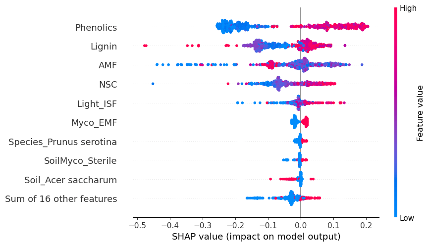
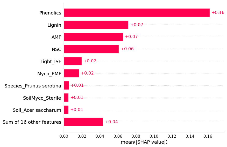
Figure 20 | Per-sample SHAP summary plot showing feature contributions for each individual observation (left), and average SHAP value plot summarizing global feature importance (right).

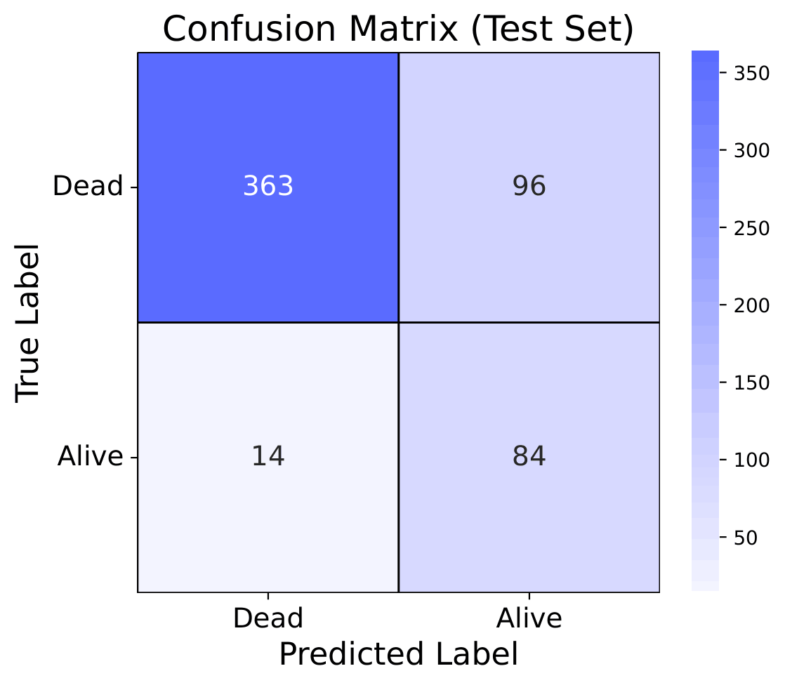
This confusion matrix in Figure 21 shows that the test results of the best performing model (Random Forest) trained on the original training dataset with class weighting approach as an example for model interpretation. The detailed evaluation metrics of the model are discussed above in Figure 14 and Table A1. The test confusion matrix shows that the chosen model performs reasonably well overall, correctly classifying 363 Dead seedlings and 84 Alive seedlings. However, it makes more errors when predicting survival: 96 individuals who were actually Dead were incorrectly predicted as Alive, while only 14 Alive individuals were misclassified as Dead. This indicates the model is better at identifying deaths than survivals, with a higher sensitivity for the Dead class but comparatively lower recall for the Alive class. In practical terms, the model tends to over-predict survival in some cases, which could be problematic in applications where failing to identify a Dead outcome carries significant consequences.

Discussion

Across the three imbalance-handling strategies—class weighting, undersampling, and oversampling—systematic differences emerged in minority-class detection, model ranking, and prediction agreement. Although all approaches aimed to correct the Alive/Dead imbalance, they shaped the training signal in different ways, which in turn affected how consistently models generalized to the unchanged test distribution and how interchangeable their predictions were across algorithms.

Under the class weighting approach, Logistic Regression, KNN, and XGBoost produced nearly identical Alive test F1 scores (52.3% ±6.4%, 53.5% ±8.4%, and 52.1% ±8.8%), while Random Forest achieved a clear gain (62.3% ±6.6%) and also led ROC AUC (88.3% ±3.4%) and PR AUC (55.6% ±10.3%). However, the wide PR AUC confide intervals across models (roughly ±9–11%) indicate that minority-class precision was unstable, consistent with the fact that weighting shifts decision boundaries without changing the underlying majority-dominated feature distribution. This helps explain why McNemar tests showed strong disagreements in accuracy outcomes—Logistic Regression was significantly worse than the other models, and even Random Forest and XGBoost differed significantly—suggesting that class weighting still allowed algorithm-specific biases to persist, with ensemble methods benefiting most from the limited minority signal.

Training on the undersampled dataset reduced this imbalance-driven separation between methods by forcing all models to learn from an explicitly balanced class distribution in the training dataset. The result was a more compressed performance landscape: Alive test F1 scores clustered between 52.5% ±6.5% and 59.8% ±6.4% (Logistic Regression to Random Forest), and ROC AUC values were tightly grouped in the mid-80% range (84.1% ±3.5% to 86.7% ±3.6%). Minority-class PR AUC was also comparable across models, with Random Forest (51.7% ±10.0%) and XGBoost (52.2% ±10.3%) modestly ahead of Logistic Regression and KNN (~44%). Importantly, McNemar testing showed that Random Forest and XGBoost were statistically indistinguishable (p = 0.6650), indicating that once the training distribution was balanced through undersampling, the two strongest models converged toward similar test-set decisions. At the same time, Logistic Regression still lagged significantly behind the others, and KNN underperformed both ensemble methods, suggesting that while undersampling narrows algorithmic differences, model capacity and decision flexibility still matter for capturing minority-class structure.

Oversampling using ADASYN produced strong minority-class metrics as well, but also amplified differences between algorithms and introduced more pronounced model-specific behavior. The Alive test F1 scores increased most for the ensemble models—Random Forest reached 59.2% ±6.8% and XGBoost peaked at 61.6% ±8.1%—while Logistic Regression and KNN remained lower (54.4% ±2.3% and 53.3% ±8.6%). Discrimination also improved for the ensembles, with Random Forest and XGBoost achieving high ROC AUC values (87.7% ±3.4% and 88.7% ±3.2%), and XGBoost producing the best Alive PR AUC (54.1% ±9.7%). Unlike undersampling, however, McNemar tests showed significant differences across nearly all pairwise comparisons, including XGBoost outperforming Random Forest (p = 0.0021) and both ensembles outperforming KNN and Logistic Regression. This pattern suggests that oversampling strengthened the minority-class signal in a way that benefited higher-capacity learners most, yielding a clearer performance ranking rather than prediction convergence. The relatively wide PR AUC confidence intervals for the minority class ( ±5-10%) also indicate that precision–recall performance remained sensitive to data splits, even as mean performance improved.

Overall, the comparison across strategies shows that the choice of imbalance mitigation influences not only average minority-class performance but also the consistency and interchangeability of model predictions. Class weighting provided moderate improvements but preserved substantial inter-model disagreement, with Random Forest emerging as the most robust option under the original distribution. Undersampling produced the greatest convergence in model behavior—most notably between Random Forest and XGBoost—suggesting it yields the most comparable predictive outcomes across strong learners, even if absolute minority-class gains were modest. Oversampling delivered the best overall minority-class performance, especially for XGBoost, but resulted in the sharpest separation between algorithms, indicating that the synthetic balancing signal amplified differences in how models exploit minority-class structure. Taken together, these results suggest that if the primary goal is maximum minority-class detection and precision–recall performance, oversampling with a high-capacity ensemble (particularly XGBoost) is most effective; if the goal is stable, method-agnostic performance with reduced dependence on model choice, undersampling provides the most consistent behavior; and if preserving the original majority-class information is critical while still improving minority detection, class weighting offers a practical compromise with Random Forest providing the most reliable results under that setting.

Compared with the Cox-model results in Wood et al. (2023), our imbalance-handling findings tell a similar story about what happens when you “tune” a system without changing the dominant structure driving outcomes [36]. In Wood et al. (2023), light availability was the strongest and most consistent predictor of seedling survival, whereas soil-source/PSF terms were generally weak and trait effects were modest and species-specific. Likewise, in our study, class weighting adjusts the loss function and can shift decision boundaries, but it does not change the underlying data structure; accordingly, minority-class performance remained moderate and uneven across algorithms, with Logistic Regression, KNN, and XGBoost showing nearly identical Alive test F1 scores (~52–54%) while Random Forest benefited most (Alive test F1 = 62.3% ±6.6%) and achieved the strongest PR AUC. In contrast, undersampling directly changes the effective training distribution and reduced differences among the strongest models, producing more comparable predictive behavior (including statistically indistinguishable accuracy between Random Forest and XGBoost by McNemar testing). Finally, oversampling with ADASYN strengthened the minority-class signal enough to yield the best overall Alive performance—particularly for XGBoost (Alive test F1 = 61.6% ±8.1%; Alive PR AUC = 54.1% ±9.7%)—but it also amplified algorithm-specific advantages, leading to a clearer performance ranking and significant disagreements across most model pairs rather than uniformly stabilizing predictions.

Limitations

A primary limitation in our study is that the data were collected under controlled conditions. Seedlings were not exposed to various environmental conditions, such as temperature fluctuations, drought, pests, or other environmental disturbances. The models’ prediction capabilities are limited to stable, relatively constant conditions. They may perform well on data similar to our  controlled setting but could struggle to generalize to other environments, where survival outcomes are driven by more complex and different factors.

The dataset is also limited to only four tree species and seven soil types. This narrow range constrains what the models can learn about species-specific and soil-dependent survival. Ecosystems include many more diverse species and soils types. Since the models were trained on only a small subset of possible species and soil types, their predictions cannot be assumed to transfer across more diverse seedlings.

In addition, the EMF feature was excluded from our analysis due to a high proportion of missing values (~54%). Including it would have required significant imputation, which could introduce additional assumptions given the size of our dataset. As a result, the fungal colonization signal learned by the models is based only on AMF, and interpretations regarding broader mycorrhizal roles should be made with caution. As a part of future work, validation of imputation approaches would allow a more rigorous assessment of mycorrhizal roles

Another limitation is related to the size and balance of the dataset. A moderate class imbalance with many more Dead than Alive seedlings introduces bias into the training. Models naturally learn more from the majority class and may end up with reduced sensitivity to minority-class patterns. This imbalance is the reason behind the variability in minority-class performance across different models.

Also, our study has temporal limitations. Measurements are taken only up to the end of the growing season. This means that the models can only predict survival within that specific time frame. Without multi-season or long-term monitoring, the models cannot predict delayed mortality or later-life survival dependencies that may occur after the first season.

Conclusions

Using a single controlled experimental dataset (one growing season; four species; seven soils), we evaluated multiple machine learning models under three data imbalance handling techniques. Under the class weighting approach, minority-class (Alive) predictions were uneven between different algorithms. Logistic Regression, KNN, and XGBoost produced almost similar Alive test F1 scores (~52–54%) while Random Forest was the strongest overall with  Alive test F1 scores of 62.3% ±6.6%. The undersampling technique reduced differences between models. Random Forest and XGBoost appeared statistically not significant in accuracy based on McNemar testing. This indicates no difference in predictive power when trained on a balanced dataset. The oversampling technique (ADASYN) achieved the strongest overall minority-class metrics. XGBoost showed the strongest performance (Alive test F1 = 61.6% ±8.1%; Alive PR AUC = 54.1% ±9.7%) and the greatest differences in accuracy between the models.

Using the best performing model trained on the original training dataset with class weighting approach, feature importance analysis with SHAP showed that chemical defense and carbon-storage traits, together with mycorrhizal associations, were key contributors to survival predictions in our dataset. Phenolics, lignin, NSC, and AMF showed the strongest positive contributions, aligning with ecological theory emphasizing defense chemistry, tissue repair capacity, and pathogen protection mediated by mutualistic fungi. In this case study, our results show that seedling survival is affected by interacting biotic and trait-based mechanisms rather than single factor. This illustrates how machine learning can support ecological theory by identifying which features include the most predictive information when multiple factors are considered simultaneously.

At the same time, our conclusions should be interpreted limited to our case study. Note that observations were collected under controlled conditions, included a limited set of species and soils, and covered only one growing season. Therefore,  the models predictions of survival outcome and findings from feature importance analysis transfer to other forests and environmental conditions remains untested. Future work should extend this approach to broader species and soil types, and multi-season monitoring.  It would be beneficial to incorporate other environmental factors (e.g., drought and temperature variability) to evaluate models performance. Overall, this case study provides evidence that  nonlinear models with appropriate imbalance handling techniques can produce useful predictions and generate testable hypotheses for broader reforestation and forest management forecasting efforts.

Appendix

Model	Train/Test	Label	Precision	Recall	F1	ROC AUC	PR AUC	Samples
Logistic Regression class_weight = “balanced”	CV Train	Alive	38.2% ± 2.1%	94.9% ± 3.4%	54.4% ± 2.3%	83.4% ± 2.5%	39.8% ± 5.2%	393
		Dead	98.4% ± 1.0%	67.0% ± 2.8%	79.7% ± 1.9%			1833
	Test	Alive	36.3% ± 5.9%	93.9% ± 4.9%	52.3% ± 6.4%	84.0% ± 3.6%	43.1% ± 9.0%	98
		Dead	98.0% ± 1.6%	64.9% ± 4.5%	78.1% ± 3.4%			459
KNN Model n_neighbors = 5 weights = “uniform” distance = “minkowski”	CV Train	Alive	50.1% ± 5.4%	53.9% ± 7.9%	51.8% ± 4.3%	84.8% ± 2.0%	48.7% ± 3.9%	393
		Dead	90.0% ± 1.3%	88.4% ± 2.9%	89.2% ± 1.4%			1833
	Test	Alive	50.4% ± 9.5%	57.2% ± 9.9%	53.5% ± 8.4%	84.5% ± 4.1%	47.7% ± 9.2%	98
		Dead	90.6% ± 2.8%	88.0% ± 3.1%	89.3% ± 2.1%			459
Random Forest class_weight = “balanced” max_features = 16 min_samples_split = 55 n_estimators = 500	CV Train	Alive	47.4% ± 3.8%	85.3% ± 6.2%	60.9% ± 3.7%	89.5% ± 1.4%	61.3% ± 5.7%	393
		Dead	96.2% ± 1.5%	79.7% ± 3.5%	87.1% ± 2.0%			1833
	Test	Alive	47.5% ± 7.0%	90.9% ± 5.6%	62.3% ± 6.6%	88.3% ± 3.4%	55.6% ± 10.3%	98
		Dead	97.6% ± 1.5%	78.5% ± 3.6%	87.0% ± 2.3%			459
XGBoost colsample_bytree = 0.6 learning_rate = 0.2 n_estimators = 100 scale_pos_weight = 1 subsample = 0.7	CV Train	Alive	57.8% ± 6.1%	52.7% ± 7.7%	55.0% ± 4.5%	88.9% ± 1.5%	59.8% ± 5.7%	393
		Dead	90.1% ± 1.3%	91.7% ± 2.4%	90.9% ± 1.1%			1833
	Test	Alive	53.6% ± 10.0%	50.9% ± 10.1%	52.1% ± 8.8%	86.1% ± 3.9%	51.8% ± 10.1%	98
		Dead	89.7% ± 2.7%	90.6% ± 2.7%	90.1% ± 2.0%			459

Model	Train/Test	Label	Precision	Recall	F1	ROC-AUC	PR-AUC	Samples
Logistic Regression	CV Train	Alive	73.8% ± 3.0%	94.1% ± 3.4%	82.7% ± 2.2%	82.6% ± 4.2%	75.1% ± 7.5%	393
		Dead	91.9% ± 4.2%	66.5% ± 5.4%	77.2% ± 3.5%			393
	Test	Alive	36.6% ± 6.2%	92.8% ± 5.1%	52.5% ± 6.5%	84.1% ± 3.5%	44.7% ± 8.9%	98
		Dead	97.7% ± 1.6%	65.7% ± 4.2%	78.5% ± 3.1%			459
KNN Model n_neighbors = 5 weights = “uniform” distance = “minkowski”	CV Train	Alive	75.9% ± 4.5%	89.4% ± 4.9%	82.0% ± 3.1%	84.5% ± 3.5%	78.0% ± 4.5%	393
		Dead	87.2% ± 4.7%	71.5% ± 7.4%	78.5% ± 4.4%			393
	Test	Alive	40.2% ± 6.6%	87.9% ± 6.4%	55.1% ± 6.7%	84.3% ± 3.6%	43.7% ± 7.8%	98
		Dead	96.5% ± 1.9%	72.0% ± 4.2%	82.4% ± 2.9%			459
Random Forest class_weight = “balanced” max_features = 22 min_sample_split = 40 n_estimators = 100	CV Train	Alive	76.6% ± 4.5%	88.4% ± 5.2%	82.0% ± 3.6%	88.3% ± 3.2%	87.1% ± 4.6%	393
		Dead	86.4% ± 5.6%	72.8% ± 7.2%	78.9% ± 4.3%			393
	Test	Alive	44.6% ± 6.5%	90.9% ± 5.9%	59.8% ± 6.4%	86.7% ± 3.6%	51.7% ± 10%	98
		Dead	97.5% ± 1.7%	76.0% ± 3.9%	85.4% ± 2.6%			459
XGBoost colsample_bytree = 0.7 learning_rate = 0.02 n_estimators = 500 scale_pos_weight = 1 subsample = 0.9	CV Train	Alive	78.2% ± 4.7%	87.6% ± 4.9%	82.6% ± 3.3%	88.8% ± 3.0%	87.0% ± 3.9%	393
		Dead	86.0% ± 4.5%	75.4% ± 6.7%	80.3% ± 4.7%			393
	Test	Alive	40.8% ± 6.6%	84.8% ± 7.2%	55.0% ± 6.6%	85.9% ± 4.0%	52.2% ± 10.3%	98
		Dead	95.8% ± 2.2%	73.7% ± 4.1%	83.3% ± 2.9%			459

Model	Train/Test	Label	Precision (%)	Recall (%)	F1 (%)	ROC-AUC	PR-AUC	Samples
Logistic Regression	Train	Alive	38.2% ± 2.1%	94.9% ± 3.4%	54.4% ± 2.3%	83.4% ± 2.5%	39.8% ± 5.2%	1833
		Dead	98.4% ± 1.0%	67.0% ± 2.8%	79.7% ± 1.9%			1833
	Test	Alive	38.2% ± 2.1%	94.9% ± 3.4%	54.4% ± 2.3%	83.4% ± 2.5%	39.8% ± 5.2%	98
		Dead	98.4% ± 1.0%	67.0% ± 2.8%	79.7% ± 1.9%			459
KNN Model n_neighbors = 5 weights = “uniform” distance = “minkowski”	Train	Alive	50.1% ± 5.4%	53.9% ± 7.9%	51.8% ± 4.3%	84.8% ± 2.0%	48.7% ± 3.9%	1833
		Dead	90.0% ± 1.3%	88.4% ± 2.9%	89.25% ± 1.4%			1833
	Test	Alive	50.3% ± 9.6%	56.8% ± 9.7%	53.3% ± 8.6%	84.3% ± 3.9%	47.5% ± 9.0%	1833
		Dead	90.5% ± 2.7%	88.0% ± 2.8%	89.2% ± 2.1%			459
Random Forest class_weight = “balanced” max_features = 1 min_samples_split = 40 n_estimators = 500	CV Train	Alive	50.4% ± 4.6%	81.0% ± 5.8%	62.0% ± 4.2%	89.5% ± 1.7%	60.9% ± 5.9%	1833
		Dead	95.3% ± 1.2%	82.8% ± 3.2%	88.6% ± 1.8%			1833
	Test	Alive	47.2% ± 7.4%	79.8% ± 8.2%	59.2% ± 6.8%	87.7% ± 3.4%	52.8% ± 9.9%	98
		Dead	94.9% ± 2.1%	80.8% ± 3.5%	87.3% ± 2.2%			459
XGBoost colsample_bytree = 0.8 learning_rate = 0.3 n_estimators = 1000 scale_pos_weight = 20 subsample = 0.9	CV Train	Alive	53.1% ± 4.6%	66.9% ± 7.1%	59.1% ± 5.0%	88.7% ± 1.7%	60.0% ± 5.9%	1833
		Dead	92.5% ± 1.4%	87.3% ± 2.8%	89.8% ± 1.3%			1833
	Test	Alive	55.5% ± 9.0%	69.5% ± 9.2%	61.6% ± 8.1%	88.7% ± 3.2%	54.1% ± 9.7%	98
		Dead	93.1% ± 2.4%	88.1% ± 3.1%	90.5% ± 2.0%			459

References 

1. Elith, J., and J. Franklin. “Species Distribution Modeling.” Reference Module in Life Sciences, 2017, https://doi.org/10.1016/b978-0-12-809633-8.02390-6 [↩]
2. Cadotte, M. W., C. A. Arnillas, S. W. Livingstone, and S. L. E. Yasui. “Predicting communities from functional traits.” Trends in Ecology & Evolution, vol. 30, no. 9, 2015, pp. 510-511 [↩]
3. Crawford KM, Bauer JT, Comita LS, Eppinga MB, Johnson DJ, Mangan SA, Queenborough SA, Strand AE, Suding KN, Umbanhowar J, Bever JD. “When and where plant-soil feedback may promote plant coexistence: a meta-analysis.” Ecology Letters, vol. 22, no. 8, 2019, pp. 1274-1284 [↩]
4. McGill, B. J., B. J. Enquist, E. Weiher, and M. Westoby. “Rebuilding community ecology from functional traits.” Trends in Ecology & Evolution, vol. 21, no. 4, 2006, pp. 178-185 [↩]
5. Van der Putten WH, Bardgett RD, Bever JD, Bezemer TM, Casper BB, Fukami T, Kardol P, Klironomos JN, Kulmatiski A, Schweitzer JA, Suding KN. “Plant–soil feedbacks: the past, the present and future challenges.” Journal of Ecology, vol. 101, no. 2, 2013, pp. 265-276 [↩]
6. Yang, Jie, Min Cao, and Nathan G. Swenson. “Why functional traits do not predict tree demographic rates.” Trends in Ecology & Evolution, vol. 33, no. 5, 2018, pp. 326-336 [↩]
7. Bever, James D., Kristi M. Westover, and Janis Antonovics. “Incorporating the soil community into plant population dynamics: the utility of the feedback approach.” Journal of Ecology, 1997, pp. 561-573 [↩]
8. Bever JD, Dickie IA, Facelli E, Facelli JM, Klironomos J, Moora M, Rillig MC, Stock WD, Tibbett M, Zobel M. “Rooting theories of plant community ecology in microbial interactions.” Trends in Ecology & Evolution, vol. 25, no. 8, 2010, pp. 468-478 [↩]
9. Jiang J, Abbott KC, Baudena M, Eppinga MB, Umbanhowar JA, Bever JD. “Pathogens and mutualists as joint drivers of host species coexistence and turnover: implications for plant competition and succession.” The American Naturalist, vol. 195, no. 4, 2020, pp. 591-602. [↩]
10. Wipf D, Krajinski F, van Tuinen D, Recorbet G, Courty PE. “Trading on the arbuscular mycorrhiza market: from arbuscules to common mycorrhizal networks.” New Phytologist, vol. 223, no. 3, 2019, pp. 1127-1142. [↩]
11. Bennett JA, Maherali H, Reinhart KO, Lekberg Y, Hart MM, Klironomos J. “Plant-soil feedbacks and mycorrhizal type influence temperate forest population dynamics.” Science, vol. 355, no. 6321, 2017, pp. 181-184. [↩]
12. Chen L, Swenson NG, Ji N, Mi X, Ren H, Guo L, Ma K. “Differential soil fungus accumulation and density dependence of trees in a subtropical forest.” Science, vol. 366, no. 6461, 2019, pp. 124-128. [↩]
13. Liang MinXia LM, Liu XuBing LX, Gilbert GS, Zheng Yi ZY, Luo Shan LS, Huang FengMin HF, Yu ShiXiao YS. “Adult trees cause density-dependent mortality in conspecific seedlings by regulating the frequency of pathogenic soil fungi.” Ecology Letters, vol. 19, no. 12, 2016, pp. 1448-1456. [↩]
14. Borowicz VA. “Do arbuscular mycorrhizal fungi alter plant–pathogen relations?” Ecology, vol. 82, no. 11, 2001, pp. 3057-3068. [↩]
15. Laliberté E, Lambers H, Burgess TI, Wright SJ. “Phosphorus limitation, soil-borne pathogens and the coexistence of plant species in hyperdiverse forests and shrublands.” New Phytologist, vol. 206, no. 2, 2015, pp. 507-521. [↩]
16. Violle C, Navas ML, Vile D, Kazakou E, Fortunel C, Hummel I, Garnier E. “Let the concept of trait be functional!” Oikos, vol. 116, no. 5, 2007, pp. 882-892. [↩]
17. Ichihara, Yu, and Keiko Yamaji. “Effect of light conditions on the resistance of current-year Fagus crenata seedlings against fungal pathogens causing damping-off in a natural beech forest: fungus isolation and histological and chemical resistance.” Journal of Chemical Ecology, vol. 35, no. 9, 2009, pp. 1077-1085. [↩]
18. Augspurger C.K. “Spatial patterns of damping-off disease during seedling recruitment in tropical forests.” 1990, pp. 131-144. [↩]
19. Dietze MC, Sala A, Carbone MS, Czimczik CI, Mantooth JA, Richardson AD, Vargas R. “Nonstructural carbon in woody plants.” Annual Review of Plant Biology, vol. 65, no. 1, 2014, pp. 667-687. [↩]
20. Witzell J. and Martín J.A. “Phenolic metabolites in the resistance of northern forest trees to pathogens—past experiences and future prospects.” Canadian Journal of Forest Research, vol. 38, no. 11, 2008, pp. 2711-2727 [↩]
21. Macaya-Sanz D, Witzell J, Collada C, Gil L, Martin JA. “Structure of core fungal endobiome in Ulmus minor: patterns within the tree and across genotypes differing in tolerance to Dutch elm disease.” bioRxiv, 2020, 2020-06. [↩]
22. Li J, Zhang X, Luo J, Lindsey S, Zhou F, Xie H, Li Y, Zhu P, Wang L, Shi Y, He H. “Differential accumulation of microbial necromass and plant lignin in synthetic versus organic fertilizer-amended soil.” Soil Biology and Biochemistry, vol. 149, 2020, 107967. [↩]
23. Luo R, Kuzyakov Y, Zhu B, Qiang W, Zhang Y, Pang X. “Phosphorus addition decreases plant lignin but increases microbial necromass contribution to soil organic carbon in a subalpine forest.” Global Change Biology, vol. 28, no. 13, 2022, pp. 4194-4210. [↩]
24. McCarthy-Neumann S. and Ibáñez I. “Plant–soil feedback links negative distance dependence and light gradient partitioning during seedling establishment.” Ecology, vol. 94, no. 4, 2013, pp. 780-786. [↩]
25. Smith-Ramesh L.M. and Reynolds H.L. “The next frontier of plant–soil feedback research: unraveling context dependence across biotic and abiotic gradients.” Journal of Vegetation Science, vol. 28, no. 3, 2017, pp. 484-494. [↩]
26. Koorem K, Tulva I, Davison J, Jairus T, Öpik M, Vasar M, Zobel M, Moora M “Arbuscular mycorrhizal fungal communities in forest plant roots are simultaneously shaped by host characteristics and canopy-mediated light availability.” Plant and Soil, vol. 410, no. 1, 2017, pp. 259-271. [↩]
27. Liu Y. and He F. “Incorporating the disease triangle framework for testing the effect of soil-borne pathogens on tree species diversity.” Functional Ecology, vol. 33, 2019, pp. 1211–1222. [↩]
28. Bereau M, Barigah TS, Louisanna E, Garbaye J. “Effects of endomycorrhizal development and light regimes on the growth of Dicorynia guianensis Amshoff seedlings.” Annals of Forest Science, vol. 57, no. 7, 2000, pp. 725-733. [↩]
29. Shi G, Liu Y, Johnson NC, Olsson PA, Mao L, Cheng G, Jiang S, An L, Du G, Feng H. “Interactive influence of light intensity and soil fertility on root-associated arbuscular mycorrhizal fungi.” Plant and Soil, vol. 378, no. 1, 2014, pp. 173-188. [↩]
30. Konvalinková T, Jansa J. “Lights off for arbuscular mycorrhiza: on its symbiotic functioning under light deprivation.” Frontiers in Plant Science, vol. 7, 2016, 782. [↩]
31. McCarthy‐Neumann S, Kobe RK. “Conspecific and heterospecific plant–soil feedbacks influence survivorship and growth of temperate tree seedlings.” Journal of Ecology, vol. 98, no. 2, 2010, pp. 408-418. [↩]
32. McCarthy-Neumann S, Ibáñez I. “Plant–soil feedback links negative distance dependence and light gradient partitioning during seedling establishment.” Ecology, vol. 94, no. 4, 2013, pp. 780-786. [↩]
33. Ichihara Y, Yamaji K. “Effect of light conditions on the resistance of current-year Fagus crenata seedlings against fungal pathogens causing damping-off in a natural beech forest: fungus isolation and histological and chemical resistance.” Journal of Chemical Ecology, vol. 35, no. 9, 2009, pp. 1077-1085. [↩]
34. Falcioni R, Moriwaki T, de Oliveira DM, Andreotti GC, de Souza LA, Dos Santos WD, Bonato CM, Antunes WC. “Increased gibberellins and light levels promote cell wall thickness and enhance lignin deposition in xylem fibers.” Frontiers in Plant Science, vol. 9, 2018, 1391. [↩]
35. LA Rogers, C Dubos, IF Cullis, C Surman, M Poole, J Willment, SD Mansfield, MM Campbell. “Light, the circadian clock, and sugar perception in the control of lignin biosynthesis.” Journal of Experimental Botany, vol. 56, no. 416, 2005, pp. 1651-1663. [↩]
36. KEA Wood, RK Kobe, I Ibáñez, S McCarthy-Neumann. “Tree seedling functional traits mediate plant-soil feedback survival responses across a gradient of light availability.” Plos one 18.11 (2023): e0293906. [↩] [↩]
37. Kohavi R. “A study of cross-validation and bootstrap for accuracy estimation and model selection.” IJCAI, vol. 14, no. 2, 1995. [↩]
38. Hastie T. Robert Tibshirani, and Jerome Friedman. “Random forests.” The Elements of Statistical Learning: Data Mining, Inference, and Prediction, Springer, New York, 2009, pp. 587-604. [↩]
39. Kavlakoglu E. “What Is the K-Nearest Neighbors (KNN) Algorithm?” IBM, 4 Oct. 2021, www.ibm.com/think/topics/knn. [↩]
40. Breiman L. “Random forests.” Machine Learning, vol. 45, no. 1, 2001, pp. 5-32. [↩]
41. Chen T, Guestrin C. “XGBoost: A Scalable Tree Boosting System.” Cornell University, 2016. [↩]
42. Powers DM. “Evaluation: from precision, recall and F-measure to ROC, informedness, markedness and correlation.” arXiv preprint, 2020, arxiv.org/abs/2010.16061. [↩]
43. Fawcett T. “An introduction to ROC analysis.” Pattern Recognition Letters, vol. 27, no. 8, 2006, pp. 861-874. [↩]
44. Bergstra J, Bengio Y. “Random search for hyper-parameter optimization.” Journal of Machine Learning Research, vol. 13, no. 1, 2012, pp. 281-305. [↩]
45. Hastie T, Tibshirani R, Friedman J. “An Introduction to Statistical Learning.” 2009. [↩]
46. Dietterich TG.. “An experimental comparison of three methods for constructing ensembles of decision trees: Bagging, boosting and randomization.” Machine Learning, vol. 32, 1998, pp. 1-22. [↩]
47. Fabian P.. “Scikit-learn: Machine learning in Python.” Journal of Machine Learning Research, vol. 12, 2011, pp. 2825-2830. [↩]
48. He H, Garcia EA. “Learning from imbalanced data.” IEEE Transactions on Knowledge and Data Engineering, vol. 21, no. 9, 2009, pp. 1263-1284. [↩]
49. He H, Bai Y, Garcia EA, Li S. “ADASYN: Adaptive synthetic sampling approach for imbalanced learning.” 2008 IEEE International Joint Conference on Neural Networks, IEEE, 2008. [↩]
50. Lundberg SM, Lee SI. “A unified approach to interpreting model predictions.” Advances in Neural Information Processing Systems, vol. 30, 2017. [↩]