Abstract
In this study, we constructed a two-dimensional magnetostatic finite element method (FEM) model that simulates the magnetic field distribution and calculates the torque generated by an electrically excited synchronous motor (EESM). A cross-sectional model of an EESM was created, with region-specific relative magnetic permeability and equivalent current densities in the windings. Specifically, our algorithm divides the motor’s domain into first-order triangular elements and solves for the magnetic vector potential. We calculated the magnetic flux density, which is the curl of the potential, and visualized the magnetic behavior with Matplotlib. Electromagnetic torque was evaluated using the Maxwell stress tensor along circular contours inside the air gap. We validated our FEM solver against the analytical magnetic field produced by a cylindrical wire and examined mesh convergence for a motor model at several mesh size parameters. Under the assumptions of constant permeability and no magnetic saturation, the computed torque showed an approximately linear dependence on both stator current amplitude and rotor current (R2>0.999). The calculated torque ripple showed a 60° periodicity, while the torque-current fitting coefficients also varied in the same pattern. The fluctuation corresponds to the geometric symmetry of the winding layout in our simplified model. Our FEM model can predict the torque-current trends under the linear-material assumptions.
Keywords: motor, finite element method (FEM), torque, simulation, electromagnetism
Introduction
Modern electric motors include direct current (DC) and alternating current (AC) motors1,2. Among AC motors, the electrically excited synchronous motor (EESM) is widely used in electric vehicles and industrial applications due to its high efficiency, controllable torque, and magnet-free design3,4.
An EESM consists of a stator carrying AC and a rotor carrying DC. A detailed description of the structure is given5. The stator wires are connected in a specific configuration to produce a three-phase AC that generates a rotating magnetic field. The rotor produces a constant electromagnetic field and rotates synchronously with the stator field.
In practice, the irregular geometry of the motor and the varying magnetic permeability produce a complicated magnetic behavior and torque that are difficult to capture with analytical methods6,7,8. The finite element method (FEM) is therefore widely used. FEM approximates the magnetic field in the domain by dividing it into many small elements, solving the governing equations on each element, and assembling the global solutions9. Specifically, two-dimensional FEM models are commonly adopted in analyzing electrical motors as an efficient approximation of the full three-dimensional electromagnetic problem10,11. Several commercial tools are available for motor designers. For instance, MathWorks’ Simscape toolbox in MATLAB and Simulink12,13 can model DC and induction motors and design control systems by solving analytical equations. However, they do not directly solve the detailed magnetic field distribution inside the motor for torque analysis. ANSYS Maxwell provides well-established 2D and 3D FEM simulation of a complete motor. However, its high costs, hardware requirements, and long learning curve make it less accessible for many users14. Some simplified FEM tools have previously been developed as well. One of the most used simplified models is the Finite Element Method Magnetics (FEMM)15, which is an interactive FEM solver for electromagnetic or heat problems. Its simplicity makes it well suited for education and research on electrical machines. In addition, Lehikoinen et al. presented an open-source finite-element analysis library for magnetic field simulations in MATLAB, providing researchers with a flexible tool for electromagnetic analysis16.
FEMM primarily provides a graphical user interface. In contrast, in this paper, we aimed to develop a simplified and accessible two-dimensional FEM model to simulate electromagnetic behavior inside a motor and then investigate the torque response to input currents. Our study exposes mesh generation, matrix assembly, magnetic solution, and torque integration, making the algorithm easier to study or modify for educational purposes and physical interpretation.
In this study, we hypothesized that: (1) the electromagnetic torque predicted by the simplified FEM model will scale approximately linearly with stator current amplitude and rotor current under the assumption of constant permeability; (2) because the simplified stator geometry has 60° rotational symmetry, the torque ripple will show a corresponding 60° periodic dependence on rotor position. We constructed a two-dimensional finite element model of an EESM cross-section, computed the internal magnetic field distribution, and calculated the torque using the Maxwell stress tensor method. Because our model is simplified with a constant magnetic permeability with no saturation or hysteresis effects, the torque-current relationship is observed under the linear-material assumption. Real machines might show nonlinear torque-current behavior when saturation effect reduces the effective permeability at high flux density. Additionally, variations in magnetizing inductance with rotor angle are considered to cause the dynamic torque behavior. The resulting torque-current and torque-angle characteristics are used to evaluate whether the simplified FEM model can reproduce the trends expected from analytical electromagnetic theory under the assumptions used in this study.
Methods
Research Design
We conducted a computational experiment using the FEM to investigate the relationship between input currents and output torque in an EESM. Our FEM model serves as a controlled environment where motor parameters can be adjusted to observe the change in torque. This flexible algorithm allows our hypotheses to be evaluated under controlled conditions that are difficult to achieve in physical experiments.
Theoretical framework
The rotor rotates synchronously with the stator magnetic field, with an angular speed ns (in revolutions per minute) of17
The rotational speed is independent of the current amplitude but solely determined by the AC frequency fe and the number of pole pairs p. Consequently, increasing the amplitude of the input current will not influence the rotor speed but instead increases the output torque, since the input power increases: Pavg=1/2VI=I2rmsR+Tωm
where:
V – the amplitude of the input voltage,
I – the amplitude of the current,
Irms – the root mean square of the current (Irms=I/√2),
ωm – the rotational speed of the motor, in radians per second (ωₘ = nₘ · 2π · 1 min/60 s)
The existing analytical dq-axis model provides an analytical expression for the torque-current relationship. According to Reinhard, the electromagnetic torque T in an EESM can be expressed as a function of the stator currents and flux links by the equation18:
where:
p – the number of pole pairs,
Lm – the magnetizing inductance,
Ld, Lq – the direct and quadrature inductance,
id, iq – the direct and quadrature-axis components of the stator current,
ie – the excitation current in the rotor.
(The original expression in Ref.18 has been rewritten using the notation used in this study.)
EM formulation
To analyze the electromagnetic behavior of the motor, we constructed a two-dimensional model representing the cross-sectional plane of a simplified EESM. We applied FEM to compute the magnetic field distribution and evaluate the electromagnetic torque under different stator current amplitudes.
Regions with different materials were assigned corresponding relative magnetic permeabilities and current densities. The FEM was then used to compute the magnetic field distribution within the domain.
The computational domain was discretized into triangular elements, with finer meshes applied in regions where stronger magnetic field variations were expected. For each element, Maxwell’s equations governing magnetostatic fields were transformed into matrix form using the Galerkin weighted residual method19. We assembled the element matrices into a global stiffness matrix representing the entire computational domain. By solving this system of equations, the magnetic vector potential and the resulting magnetic field distribution across the motor cross-section were obtained.
The magnetic field in the motor cross-section is the curl of the magnetic vector potential20. In a two-dimensional magnetostatic problem, the magnetic vector potential A has only a z-component, and the magnetic flux density B can be obtained as:
Substituting this expression into the Maxwell-Ampere law ∇×B=−μJ:
where µ is the magnetic permeability and J is the current density.
This governing equation was solved using the FEM, where the domain was discretized into triangular elements. We transformed the differential equation into a matrix equation for all elements21,22 using the Galerkin weighted residual method19. These element matrices were then assembled into a global stiffness matrix representing the entire domain:
where Anodes is the magnetic potential at the nodes.
Therefore, after assembling the stiffness matrix S and the load vector T of all elements and solving the total equation, we can derive the magnetic potential over the region.
Because this system is still singular, Dirichlet boundary19 conditions are added by fixing the magnetic potential along the outer boundary of the domain at zero, which means the magnetic field can hardly leak into the surrounding air. This boundary condition is appropriate for the present geometry because the outer boundary is placed outside the stator, while the main torque-producing field is concentrated in the rotor, stator, and narrow air gap. A larger surrounding air domain would provide a more accurate open-boundary approximation, but this minor improvement was not pursued.
In our model, the dominant magnetic flux is confined within the high-permeability stator and rotor cores (µr = 2000.0), while the magnetic field near the outer boundary is comparatively weak. Consequently, the imposed boundary condition is expected to have only a limited influence on the magnetic field distribution in the air gap and on the calculated electromagnetic torque. The final magnetic field is the curl of the magnetic potential: B=∇×A.
Numerical implementation
The FEM algorithm was implemented in Python. The motor cross-section was meshed using Gmsh modelling software, which provides a Python API for generating two-dimensional meshes23. The mesh contains the coordinates of all nodes and the connectivity of the triangular elements.
The FEM solver was implemented in Python using meshes generated by Gmsh. Sparse matrices (scipy.sparse)24 are used to reduce memory usage and calculation time.
Validation of the FEM solver
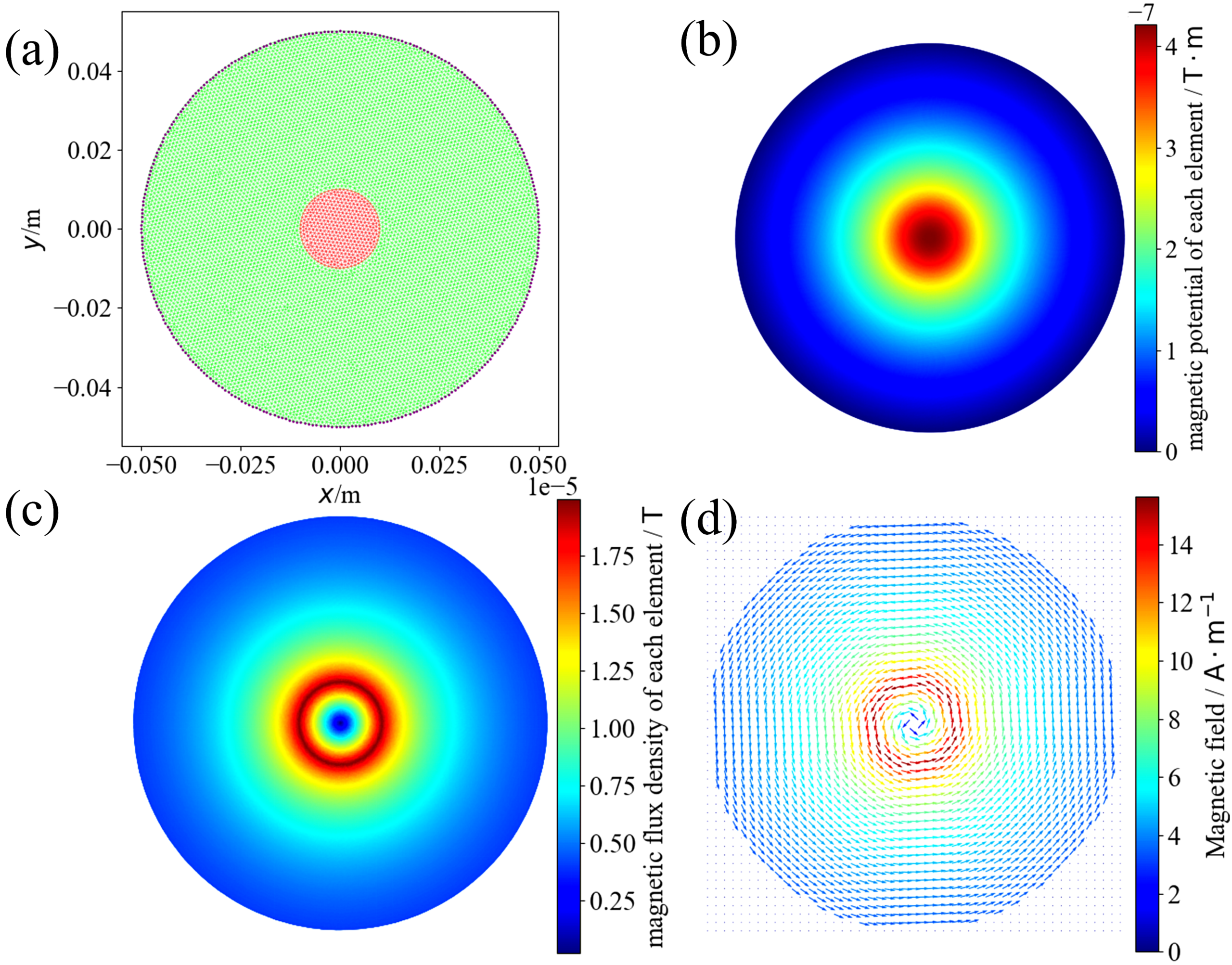
To verify the numerical formulation, we constructed a benchmark problem: a circular domain (radius 0.05 m, green) with a straight circular wire (radius 0.01 m, red) at the center, as shown in Fig. 1(a). The dimensions were chosen for numerical convenience and field visualization rather than representing a practical conductor geometry, and a current of 1 A was assigned to enhance the contrast ratio of the magnetic field pattern, leading to a current density J of 1/(π · 0.01²) ≈ 3183.099 A/m². In addition, both wires and surrounding materials used in the validation were assigned the same relative magnetic permeability of 1.0 for visibility of the field inside the wire. Its mesh is generated using Gmsh, with finer elements near the wire to capture strong magnetic field gradients. The simulation results were visualized using Matplotlib25.
The mesh was processed by the “Mesh” class, which applied FEM to the mesh and calculated magnetic field distributions. Fig. 1 demonstrates the results of the computation. The magnetic potential induced by the wire has only a z-component because it is perpendicular to the plane. The distribution of the magnetic potential is shown in Fig. 1(b). The magnetic field can be obtained by calculating the curl of the potential (∇×A).
To quantitatively validate the FEM implementation, the numerical solution was compared with the analytical magnetic field distribution of a cylindrical current-carrying conductor. The analytical solution is represented by:
where:
r – the distance from the center,
R – the radius of the wire (0.01 m),
I – the current in the wire (1.0 A).
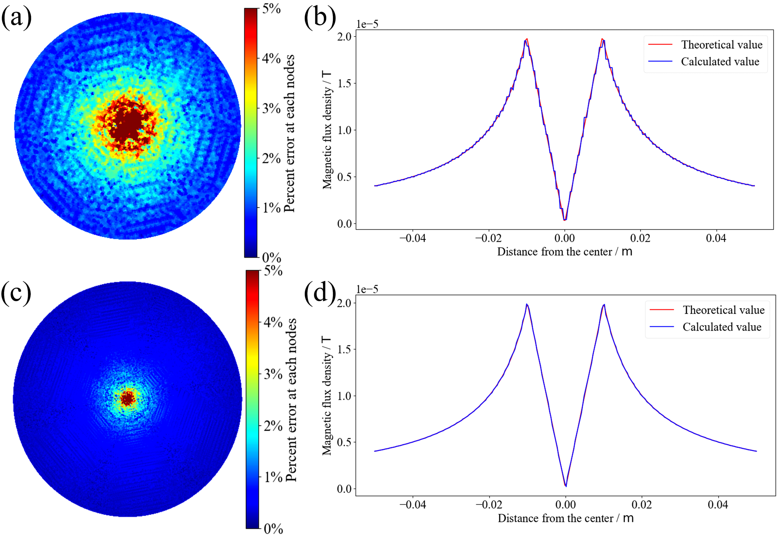
The magnitude of the magnetic field shown in Fig. 1(c) is consistent with the analytical solution, as it is strongest along the edges of the wire, decreasing linearly toward the center and inversely proportional to the radial distance outwards. In Fig. 1(d), the magnetic field vectors circulate in a counterclockwise direction, consistent with the right-hand rule. Notably, the field goes along the outside boundary due to the boundary condition of setting the potential to 0. The errors of the two mesh resolutions are listed in Table 1, and the relative error distribution is shown in Fig. 2.
The distribution of percentage errors and the comparison of the simulated and analytical results are shown above. Our FEM algorithm has low errors from the theoretical derivation and correctly solves the magnetostatic field equations. When the mesh size was reduced from 0.001 m to 0.0003 m, the mean percent error decreased from 1.61% to 0.50%, while the relative L2 error decreased from 3.11% to 0.95%. The RMSE was reduced by approximately 70%. These results indicate that the FEM algorithm converges toward the analytical solution as the mesh is refined.
| Mesh Size (m) | Mean % Error | Mean Abs. Error (T) | Max Abs. Error (T) | L2 Error | RMSE (T) |
| 0.0010 | 1.61% | 1.37 × 10⁻⁷ | 1.30 × 10⁻⁶ | 3.11% | 2.40 × 10⁻⁷ |
| 0.0003 | 0.50% | 4.22 × 10⁻⁸ | 4.07 × 10⁻⁷ | 0.95% | 7.32 × 10⁻⁸ |
Motor model configuration
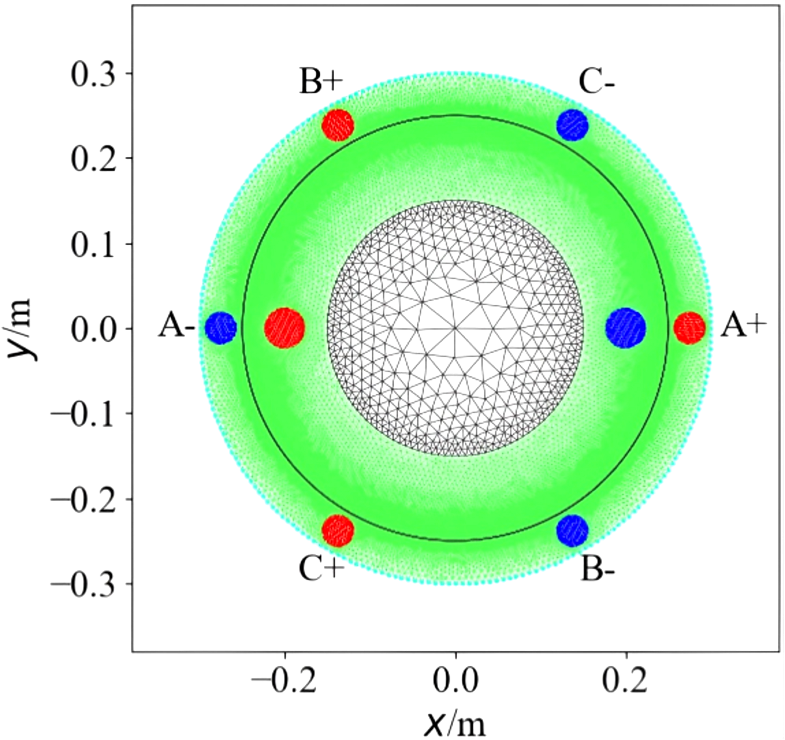
The sample in this computational study consists of a simulated two-dimensional cross-sectional model of an EESM. Using the Gmsh Python API, a two-dimensional model of a three-phase three-slot EESM was created, shown in Fig. 3.
The mesh resolution was refined in the air-gap region (the thin black area between the two green layers) to improve the accuracy of the torque calculation. In the motor model:
The outer radius of the stator: 0.300 m,
The inner radius of the stator: 0.250 m,
The rotor radius: 0.247 m, The air-gap width: 0.003 m.
The inner part of the rotor contains a hollow air space (radius 0.150 m) to reduce magnetic flux leakage through the center26 and improve the magnetic flux path.
The dimensions used in this study were selected to create a geometrically simple benchmark problem suitable for educational FEM analysis.
The primary objective of the model was not to reproduce the performance of a specific commercial motor but rather to investigate qualitative relationships between magnetic field distribution, input current, rotor position, and electromagnetic torque. The rotor windings carry direct current, while the stator windings carry alternating currents. Table 2 presents some more detailed data about the wires and currents:
| Quantity | Stator | Rotor |
| Equivalent Winding Radius | 0.020 m | 0.025 m |
| Turns | 5 | 50 |
| Current per Turn | Is = 800 A | Ir = 200 A |
| Assigned Current Density | Js = 3.183×10⁶ A/m2 | Jr = 5.093×10⁶ A/m2 |
| Distance from Center | 0.257 m | 0.200 m |
These values were selected to produce magnetic field magnitudes suitable for numerical visualization and torque analysis.
The stator windings were denoted with three pole pairs: A+/A−, B+/B−, and C+/C−. For each phase, the positive and negative regions denote current flowing out of and into the two-dimensional plane, respectively. The three-phase currents were described as a balanced three-phase set:
where Iₛ represents the AC amplitude, and φₑ = φₑ₀ + ωₑt (ωₑ = 360°fₑ). Here, φₑ refers to the electrical phase angle used to define the balanced three-phase excitation. To maximize electromagnetic torque (which is discussed in 3.1), the stator phase currents are adjusted such that the resultant stator magnetic field remains approximately perpendicular to the rotor magnetic field. The resulting stator magnetic field forms an angle θms with respect to a fixed stator reference frame, while the rotor magnetic axis is denoted by θmr. The angular displacement δ = θmr-θms is referred to as the rotor-stator field angle. The current density assigned to each winding region is computed as J=NI/A. Therefore, the absolute torque values should be interpreted within the chosen equivalent-winding representation, while the focus of this study is the scaling trend with current amplitude and rotor position.
Torque calculation
The electromagnetic torque can be calculated using the Maxwell tensor method27,28. The torque acting on the rotor can be expressed as:
where:
lef – the shaft length of the motor,
r – the radius of the line integral,
Br – the radial component of the magnetic flux density in the air gap,
Bt – the tangential component of the magnetic flux density in the air gap,
θ – the angular position along the circular contour in the air gap.
In our implementation, the Maxwell stress tensor is evaluated along a circular contour in the air gap. The contour is divided into N (default 2880) equal angular differentials (dθ), where the magnetic flux density is decomposed into radial and tangential components:
According to (8) and (9), the torque can be further written as:
where where Δθ = 2π/N, while Bᵣ(θₖ) and Bₜ(θₖ) are the radial and tangential components of the magnetic flux density at the k-th angular position, respectively. As the FEM model is two-dimensional, the simulated magnetic field represents the cross-sectional field distribution of a motor assumed to be uniform along the axial direction. End effects, end windings, and axial leakage flux are neglected. The Maxwell-stress integral therefore first produces torque per unit axial length. To convert the two-dimensional Maxwell-stress result into total electromagnetic torque, an effective axial stack length of lef = 0.3 m was then used in all torque calculations. Because the model is two-dimensional, the reported torque values should be interpreted as estimates for a motor with this assumed stack length and without axial end effects.
Fig. 4 shows the variation of the calculated torque with contour radius for several mesh densities. For tested mesh sizes of 0.001 – 0.008, the torque remained relatively stable within most of the air-gap radii. Strong local fluctuations were observed when the contour intersected element-layer interfaces or approached material boundaries. These fluctuations originate from the piecewise approximation of the magnetic flux density in first-order triangular FEM and do not represent physical torque variations. Excluding the immediate vicinity of the rotor and stator boundaries, the torque varied only slightly across the stable portion of the air gap, indicating that the Maxwell-stress formulation provides a consistent torque estimate.
For an exact continuous magnetic field, the Maxwell-stress torque is independent of the contour radius if the contour remains entirely within the air gap. However, in the present FEM model, the magnetic flux density is obtained from first-order triangular elements, resulting in possible discontinuities in the magnetic field across element boundaries, making the computed torque fluctuate with the contour radius. To reduce this effect, 30 radii were sampled in the air gap, and the final torque was obtained by taking the median of these results calculated from the sampled radius because the median is resistant to outliers. This procedure minimizes the sensitivity of the Maxwell stress calculation to individual element-layer interfaces and provides a more robust estimation of the electromagnetic torque.
| Mesh Size | Median Torque (N·m) | IQR (N·m) |
| 0.001 | 412.933 | 1.220 |
| 0.003 | 412.119 | 3.946 |
| 0.005 | 410.612 | 4.785 |
| 0.008 | 408.304 | 5.655 |
| 0.010 | 397.755 | 7.078 |
| 0.030 | 346.987 | 177.268 |
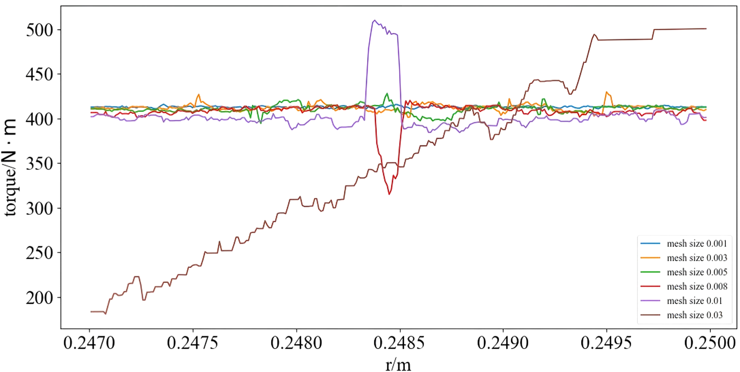
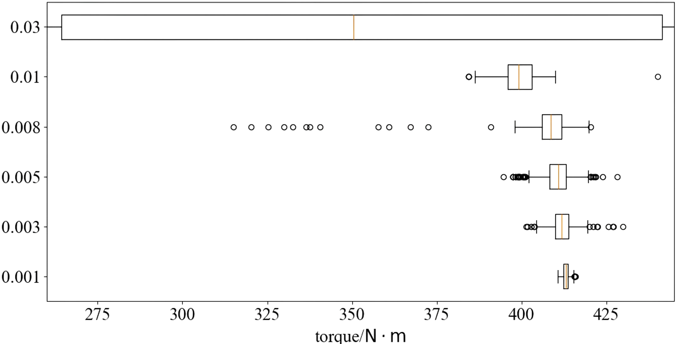
Fig. 4 and 5, together with Table 3, show the torque obtained using different mesh sizes. For mesh sizes below 0.01, the median torque remained within approximately 3% of the finest-mesh result, suggesting that the solution is convergent.
Based on the mesh convergence study, a mesh size of 0.008 was adopted in subsequent simulations, considering both accuracy and the time complexity of the algorithm.
The Python code of the FEM algorithm is available at the GitHub repository in the Appendix.
Results
Magnetic field distribution in the motor
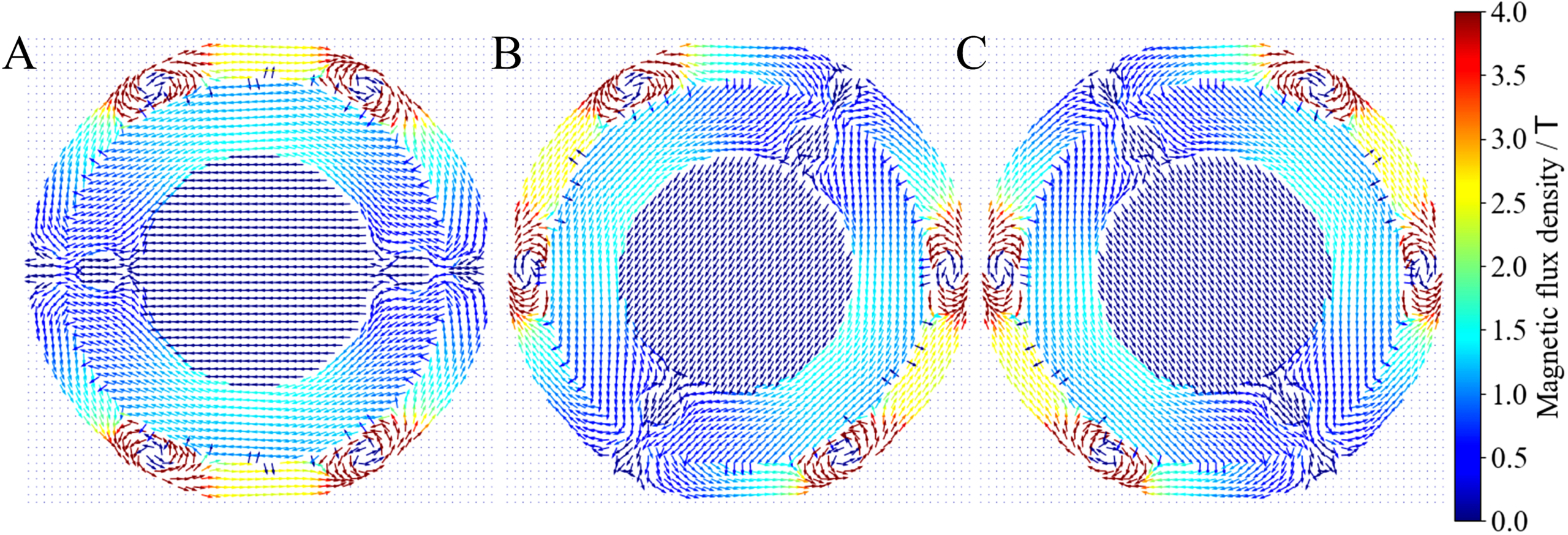
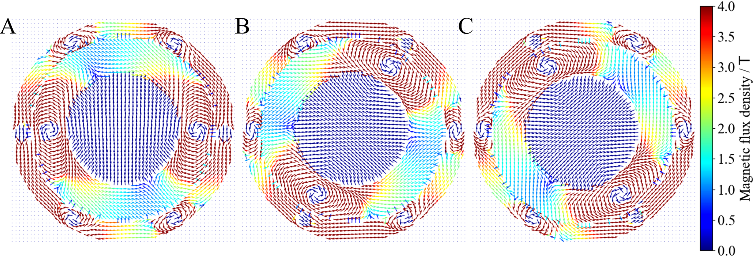
For each simulation, we computed the magnetic field distribution and electromagnetic torque under specified input conditions. Multiple simulations were conducted by varying stator current, rotor current, and rotor angle. The stator windings generated a rotating magnetic field in the stator region. Fig. 6 shows that the magnetic field rotates synchronously with the electrical phase angle φe. The brown region indicates areas where the magnetic flux density exceeds 4 T, which occur because saturation is not considered, and the relative permeability is assumed to be constant. They should be interpreted as numerical artifacts and only as relative indicators of field distribution rather than physically realistic magnitudes. In Fig. 6(a), when the phase angle φe was 0, the stator magnetic field in the rotor pointed to the left in the motor region. As φe increased by 60°, the field rotated counterclockwise by the same angle.
Torque as a function of rotor-stator field angle
In order to examine the relationship between torque and the angular displacement between the rotor and stator field, the stator field was fixed at φe=−90° while the rotor rotated, and the resulting torque was calculated.
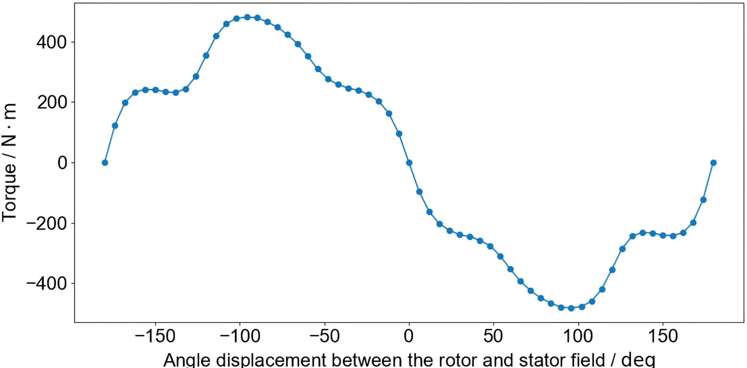
The torque was then analyzed as a function of the angular displacement between the rotor and stator magnetic fields ( δ = θmr-θms), and the result is shown in Fig. 7. The torque reached its maximum of approximately 480 N·m when the rotor field lagged the stator field by around 90°.
In all the following simulations, the rotor field was kept perpendicular to the stator field. As shown in Fig. 8, the magnetic field lines continued to follow the air-gap boundary under this condition.
Independent numerical verification using FEMM
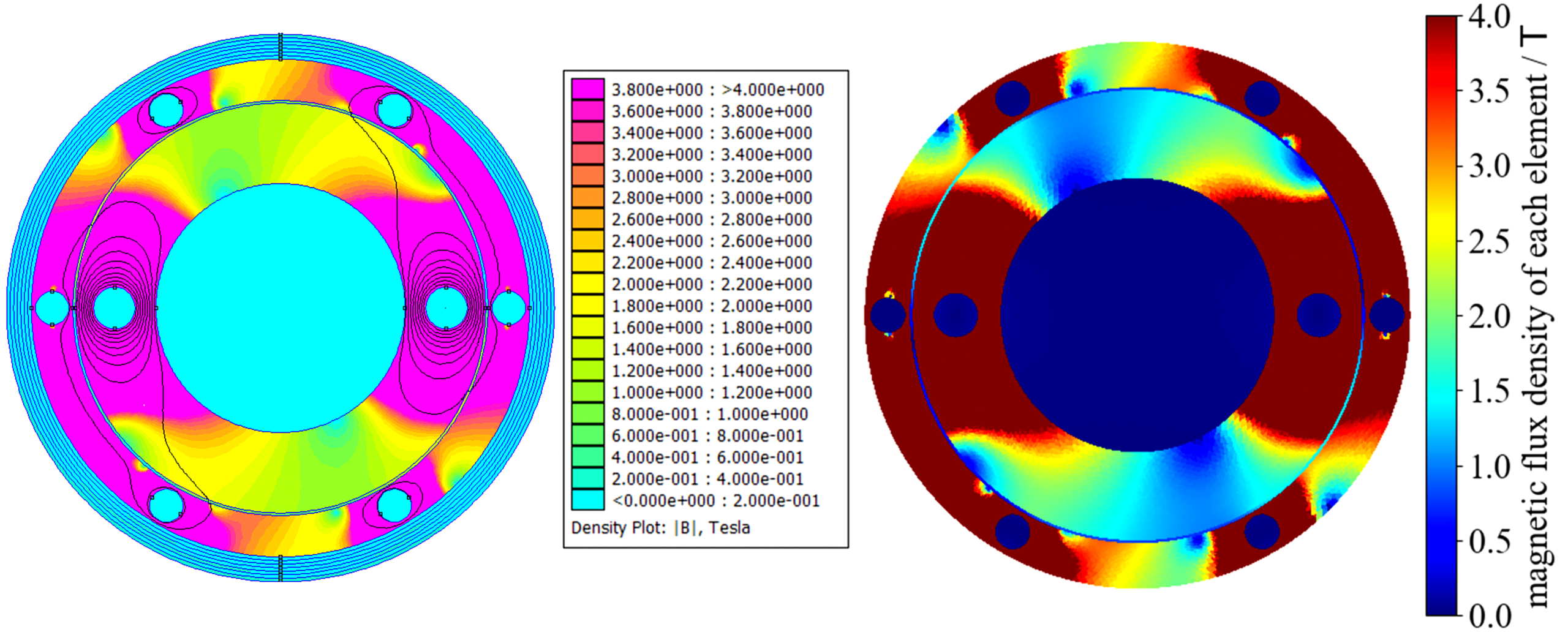
To assess the consistency of the proposed FEM implementation, the derived magnetic distribution and torque were compared with results obtained from FEMM under identical geometric configuration, excitation conditions, and Maxwell stress tensor contour integral. Both models solve the same magnetostatic governing equations using thirty circular contours distributed across the air gap. The FEMM comparison should be interpreted as an independent numerical verification of the FEM implementation rather than a validation of the physical motor model. Both approaches solve the same two-dimensional magnetostatic problem under identical linear-material assumptions, so they share the same modeling limitations, neglecting magnetic saturation, hysteresis, end effects, and axial leakage flux.
| Model | Nodes | Elements | Median Torque (N·m) | Torque IQR (N·m) | Solving Time (s) |
| FEMM | 24141 | 47920 | 414.961 | 8.308 | 2.155 |
| Present | 24573 | 48908 | 408.304 | 5.215 | 2.228 |
The reported value corresponds to the median torque, while the interquartile range (IQR) was used to quantify contour-radius sensitivity. Table 4 summarizes the mesh statistics and torque results obtained from FEMM and the present algorithm. Under the baseline operating condition, the proposed FEM model predicts a median torque of approximately 408.304 N·m, while FEMM yields approximately 414.961 N·m, corresponding to a relative error in average torque of 1.604%.
This close agreement indicates that the Maxwell-stress contour integration procedure implemented in the present FEM algorithm produces results consistent with those from an established FEM solver. The remaining difference is likely attributable to discrepancies in mesh topology, air-gap discretization, and field interpolation during contour integration.
Torque dependence on stator current amplitude and rotor current
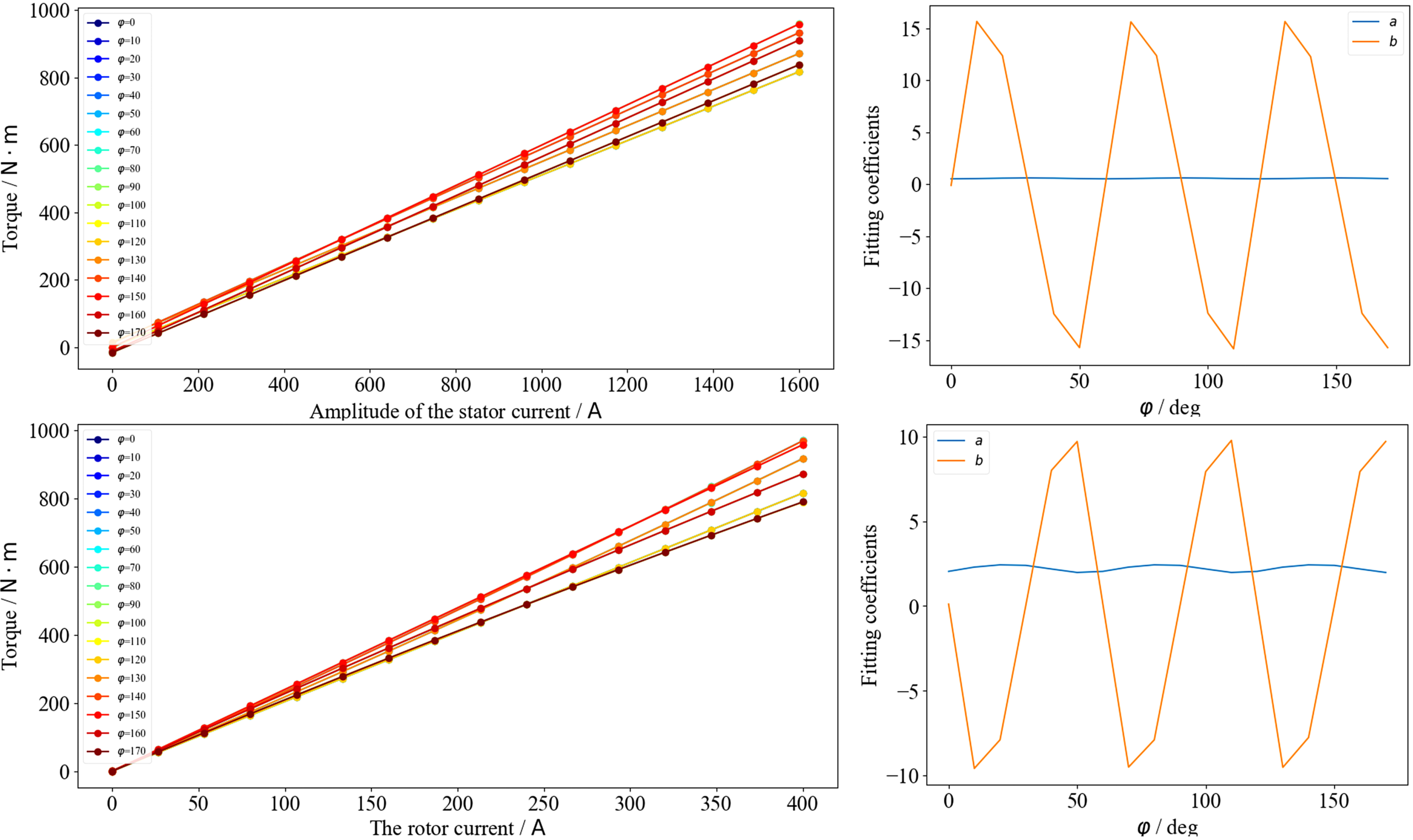
To examine how torque depends on stator current, the rotor current was fixed at 200 A, and fifteen stator current amplitudes ranging from 0 to 1600 A were tested.
For each current amplitude, we performed the simulations phase angles φe from 0° to 170° in 10° increments. The relationship between the stator current amplitudes and the output torques was then analyzed.
To examine the influence of rotor current, the stator current amplitude was fixed at 800 A. Fifteen rotor current amplitudes ranging from 0 to 400 A were tested for the same set of phase angles. Fig. 10(c) shows a similar linear relationship between the output torque and the rotor current.
Linear regression was performed for the torque-current curve at each rotor position, and the results are shown in Table 5 and 6. The coefficient of determination (R2) exceeded 0.99999998 for all fitted datasets, indicating a strong linear relationship between torque and current within the constant-permeability model.
The fitted slopes varied periodically with rotor position. Fig. 10(d) describes the variation of the fitted slopes with rotor position. This periodic variation is approximately symmetric every 60°, consistent with the stator geometry. The periodic variation of the fitted torque-current coefficient is consistent with a periodic modulation of the effective electromagnetic coupling between the stator and rotor. This may partially explain the calculated torque ripple.
| Electric angle φe | Slope (N·m/A) | 95% CI | R2 |
| 0° | 0.508 | (0.508, 0.508) | 0.999999987638150 |
| 30° | 0.597 | (0.597, 0.597) | 0.999999999998387 |
| 60° | 0.508 | (0.508, 0.508) | 0.999999991225648 |
| 90° | 0.597 | (0.597, 0.597) | 0.999999999999282 |
| 120° | 0.508 | (0.508, 0.508) | 0.999999987714331 |
| 150° | 0.597 | (0.597, 0.597) | 0.999999999998628 |
| Electric angle φe | Slope (N·m/A) | 95% CI | R2 |
| 0° | 2.032 | (2.032, 2.032) | 0.999999999996003 |
| 30° | 2.389 | (2.389, 2.389) | 0.999999999969194 |
| 60° | 2.032 | (2.032, 2.032) | 0.999999997950806 |
| 90° | 2.389 | (2.389, 2.389) | 0.999999999979973 |
| 120° | 2.031 | (2.031, 2.031) | 0.999999989684692 |
| 150° | 2.389 | (2.389, 2.389) | 0.999999999870308 |
| Tmin (N·m) | Tmax (N·m) | Tmean (N·m) | Tpp = Tmax – Tmin (N·m) | Rripple |
| 403.059 | 479.614 | 443.400 | 76.554 | 17.265% |
Because the simplified geometry does not belong to a specific commercial motor, an independently measured value of Lm is not available. Therefore, the comparison with the classical torque equation is made at the level of functional dependence rather than absolute parameter prediction. Under the condition id = 0, the classical equation predicts a linear relationship between torque and iq(T = ³⁄₂Lₘiₑiq). With R2 > 0.99999998 for all rotor positions, our simulation showed that the output torque was directly proportional to both the input rotor current and stator current amplitude, consistent with the equation of classic motor theory. This linearity is consistent with (2), which predicts T ∝ iqie under constant inductance. Thus, we can derive the magnetizing inductance between the stator and the rotor as an effective coupling coefficient:
The same kind of test was conducted with FEMM. Fixing the stator current amplitude at 800 A, we calculated the torque under different rotor currents (100 A, 200 A, 300 A, 400 A):
| φe | FEMM slope | Our slope | Error |
| 0° | 2.091 | 2.041 | 2.384% |
| 20° | 2.457 | 2.426 | −1.237% |
| 40° | 2.151 | 2.181 | 1.416% |
Fixing the rotor at 200 A, the torque was calculated at different stator current amplitudes (400 A, 800 A, 1200 A, 1600 A):
| φe | FEMM slope | Our slope | Error |
| 0° | 0.511 | 0.511 | 0.168% |
| 20° | 0.575 | 0.575 | 0.445% |
| 40° | 0.577 | 0.577 | 0.382% |
This agreement shows that our model successfully predicts the linear relationship between the output torque and the input rotor current and stator current amplitude.
Rotor-angle-dependent torque ripple
Finally, we examined the torque as a function of rotor phase angle, while the stator current amplitude and the rotor current were kept at 800 A and 200 A, respectively. In Fig. 11, the torque was found to vary periodically with rotor phase angle, a phenomenon known as torque ripple. The ripple exhibited a period of 60°, consistent with the 60° rotational symmetry of the stator magnetic field distribution. This periodic behavior indicates that the electromagnetic coupling between the rotor and stator varies with their relative angular alignment.
The significance of the peak-to-peak magnitude relative to the mean torque can be calculated:
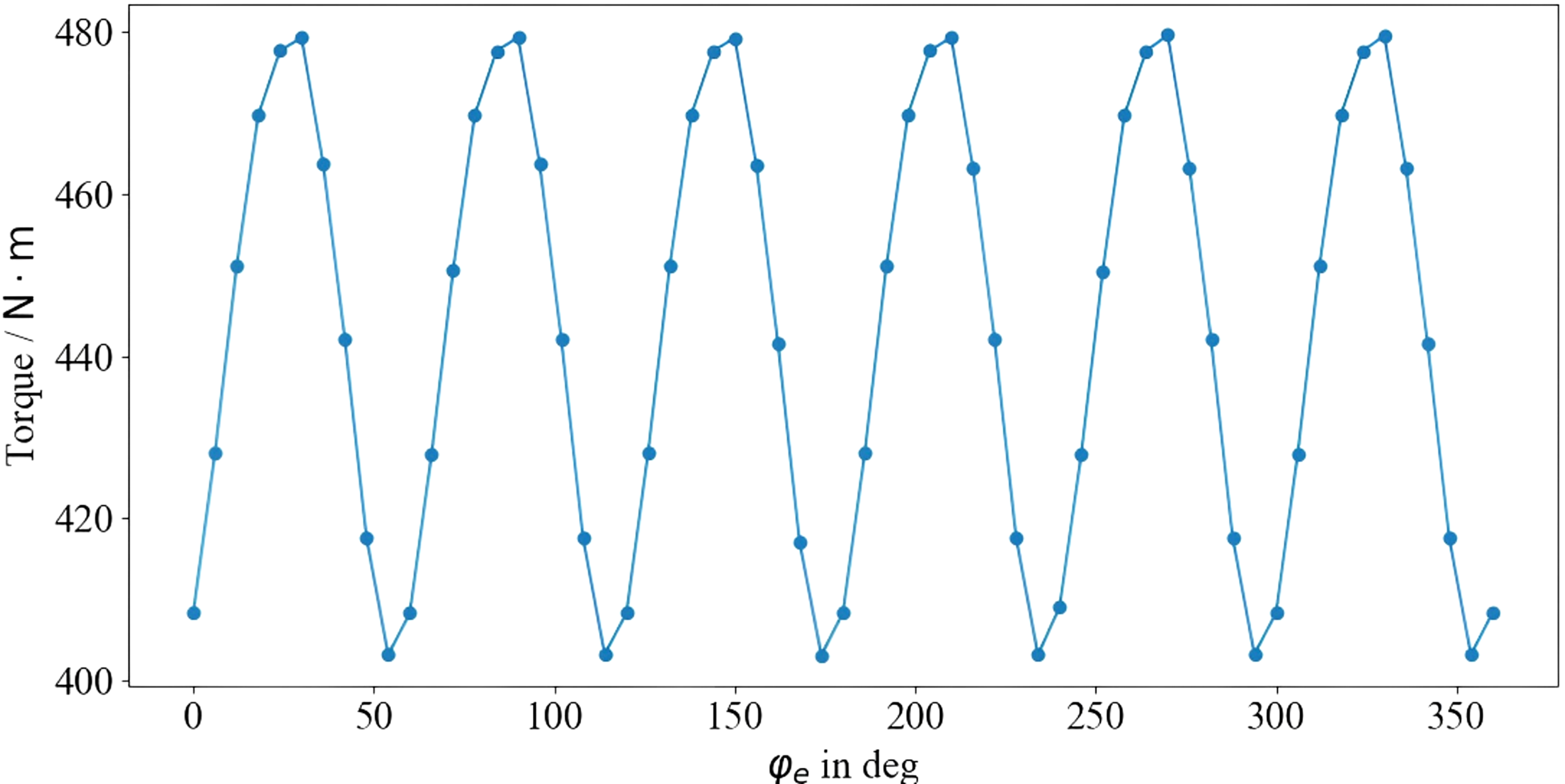
Under the baseline operating condition of Is=800 A and Ir=200 A, the mean torque was 443.400 N·m, and the peak-to-peak ripple was 76.554 N·m, leading to a ripple ratio of 17.265%. The observed ripple ratio falls in the common range for simplified slot-based machine models, even though direct comparison is difficult because the present geometry does not correspond to a specific commercial machine.
Besides, the fitted torque-current coefficients exhibit clear 60° periodicity as well. According to the analytical EESM torque equation by Reinhard18, the observed periodic variation of the fitted slope indicates a corresponding periodic variation in the magnetizing inductance between the stator and rotor wires.
In practical electrical machines, the torque ripple can lead to mechanical vibration, acoustic noise, and reduced control stability. Understanding the physical origin of torque ripple is important for improving motor performance and designing effective control strategies. The torque ripple may also originate from cogging torque, slotting effects, harmonic content of the air-gap flux density, magnetic saturation, or inverter current harmonics. The present model assumes constant permeability, idealized winding regions, and a two-dimensional geometry, so these causes of the ripple are not explicitly presented in the simplified model.
Together, these findings support both hypotheses proposed in the Introduction.
Discussion
Interpretation of the torque-current relationship
In this study, we developed a simplified two-dimensional FEM model to simulate magnetic behavior in an EESM and investigate how input currents influence the electromagnetic torque. Our FEM model produced the expected relationship between magnetic field distribution and electromagnetic torque under the assumption of no saturation. In addition, the solved magnetic field obtained from the FEM simulation reveals how the geometric structure of the motor influences the torque. The torque-current gradient varies periodically with rotor angle, demonstrating the influence of the changing electromagnetic coupling.
We used a two-dimensional cross-sectional motor model instead of a three-dimensional one for a simpler demonstration of the electromagnetic behaviors in the machine. Such models are welcomed in electrical-machine analysis because they allow the magnetic field distribution in the stator, rotor, and air-gap regions to be analyzed with substantially lower geometric complexity7,8,29.
The simulations also showed the torque ripple. This result is consistent with the 60-degree symmetric structure of the stator. It can influence motor performance in practical applications.
The proposed FEM model, FEMM simulations, and the analytical models produced consistent electromagnetic behavior of the EESM. Quantitatively, the FEM model predicts a torque of approximately 408 N·m, which deviates approximately 1.6% from the same model in FEMM. Agreement with FEMM supports the validity of our numerical implementation and torque-evaluation procedure. The difference between the two numerical implementations may arise from variations in mesh discretization, air-gap field interpolation, and the discrepancy in the evaluation of the Maxwell stress tensor.
Our simplified FEM model reproduces the expected electromagnetic mechanisms for torque generation. It demonstrates mesh generation, FEM solution, and torque calculation transparently, making it useful for educational and exploratory studies of EESMs.
Limitations
The present model is based on a two-dimensional cross-sectional representation of the motor. Therefore, several three-dimensional effects, including end-turn inductances, axial leakage flux, end fringing fields, and slot skewing effects, are neglected11,30.
These effects mainly influence the inductance and torque, while the relationship between current excitation and torque production is still primarily governed by the cross-sectional magnetic field distribution. Because no three-dimensional FEM model or experimental measurements were available in the present study, the magnitude of the resulting error could not be quantified. Consequently, our study should be interpreted more as a qualitative investigation of torque-current trends rather than a high-fidelity prediction of a specific commercial motor.
A full cross-check with the virtual work method was not conducted because the present implementation changes the mesh when creating the small angular displacement of the rotor, making the finite-difference energy derivative numerically sensitive. Instead, we strengthened the Maxwell-stress torque evaluation by using circular contours, multiple contour radii, and independent FEMM comparison.
The adopted mesh resolution represents a compromise between computational efficiency and local field accuracy, particularly near the air gap where strong magnetic gradients occur.
Commercial FEM tools such as ANSYS Maxwell and MathWorks Simscape Electrical generally include refined meshing strategies, nonlinear material models, and machine design tools with more functions. However, the primary purpose of our model is not to replicate high-fidelity industrial solvers but to provide a simplified and transparent computational tool that preserves the dominant electromagnetic coupling mechanisms while significantly reducing computational complexity. Because magnetic saturation, detailed winding structure, three-dimensional effects, and experimental validation were not included, the model should only be used for educational or exploratory purposes.
Future work could include benchmark geometries with material interfaces and narrow air gaps to further test the solver under conditions closer to electrical machines. We will also focus on improving both computational efficiency and model accuracy, including optimizing the matrix assembly process, implementing parallel or multi-threaded computation, and refining the mesh in regions with strong magnetic field gradients. These improvements could enable future comparisons with experimental measurements and three-dimensional models.
Acknowledgments
I would like to thank Professor Andy Haas for his guidance and support during my learning process in computational physics, and Doctor Chong Di for helping me understand the finite element method.
Appendix
The Python source code used for the FEM simulation is available at the GitHub repository: https://github.com/TravelerFromAbyss/Motor_model_new.
References
- A. Ben-Menahem. Historical encyclopedia of natural and mathematical sciences. Springer Science & Business Media, 2009. [↩]
- M. M. Radmanesh. The gateway to understanding: Electrons to waves and beyond. AuthorHouse, 2005. [↩]
- J. Bredthauer, B. Wachta, and S. Appleton. Synchronous Motors with Cylindrical Rotors for the Petrochemical Industry. IEEE Transactions on Industry Applications. Vol. IA-23, pg. 451–463, 1987, https://doi.org/10.1109/TIA.1987.4504932. [↩]
- G. Mademlis, Y. Liu, J. Tang, L. Boscaglia, and N. Sharma. Performance Evaluation of Electrically Excited Synchronous Machine compared to PMSM for High-Power Traction Drives. 2020 International Conference on Electrical Machines (ICEM). pg. 1793–1799, 2020, https://doi.org/10.1109/ICEM49940.2020.9270852. [↩]
- N. Thi and N. Dung. An Overview on Electric Motors: Classification, Control and Applications. International Journal of Research and Scientific Innovation. Vol. 2321-2705, pg. 318–333, 2024, https://doi.org/10.51244/IJRSI.2024.11110025. [↩]
- P. C. Krause, O. Wasynczuk, and S. D. Sudhoff. Analysis of Electric Machinery and Drive Systems. Wiley, 2025, https://doi.org/10.1002/9781394293896. [↩]
- J. Pyrhonen, T. Jokinen, and V. Hrabovcova. Design of Rotating Electrical Machines. Wiley, 2014, https://doi.org/10.1002/9781118701591. [↩] [↩]
- S. J. Salon. Finite Element Analysis of Electrical Machines. Springer, 1995. [↩] [↩]
- J. N. Reddy. An introduction to the finite element method. McGraw-Hill Education, 2006. [↩]
- M. Mirzaei and R. Mirjalili. 2D Analysis of Solid Iron Rotor Induction Machines. 2025 24th International Symposium INFOTEH-JAHORINA (INFOTEH). pg. 1–5, 2025, https://doi.org/10.1109/INFOTEH64129.2025.10959276. [↩]
- S. Naik, B. Bag, and K. Chandrasekaran. A 2D and 3D Analysis on Electromagnetic Parameters of Spoke-shape Interior Permanent Magnet Synchronous Motor Using FEM. Periodica Polytechnica Electrical Engineering and Computer Science. Vol. 67, pg. 181–193, 2023, https://doi.org/10.3311/PPee.20835. [↩] [↩]
- The MathWorks, Inc. Simscape User’s Guide, Version R2026x. The MathWorks, Inc. Natick, MA, 2026. https://mathworks.com. [↩]
- The MathWorks, Inc. Simulink User’s Guide, Version R2026x. The MathWorks, Inc. Natick, MA, 2026. https://mathworks.com. [↩]
- Ansys, Inc. Ansys Maxwell, Release 2026 R1. Ansys, Inc. Canonsburg, PA, 2026. https://www.ansys.com/products/electronics/ansys-maxwell. [↩]
- D. C. Meeker. Finite Element Method Magnetics. 4.2. FEMM. Natick, MA, 2018. http://www.femm.info [↩]
- A. Lehikoinen, T. Davidsson, A. Arkkio, and A. Belahcen. A High-Performance Open-Source Finite Element Analysis Library for Magnetics in MATLAB. 2018 XIII International Conference on Electrical Machines (ICEM). pg. 486–492, 2018, https://doi.org/10.1109/ICELMACH.2018.8507235. [↩]
- S. J. Chapman. Electric machinery fundamentals. McGraw-Hill, 2003. [↩]
- J. Reinhard, K. Lohe, and K. Graichen. Optimal current setpoint computation for externally excited synchronous machines. 2022 IEEE Conference on Control Technology and Applications (CCTA). pg. 1319–1326, 2022, https://doi.org/10.1109/CCTA49430.2022.9965988. [↩] [↩] [↩]
- A. Ern and J.-L. Guermond. Theory and practice of finite elements. Springer Science & Business Media, 2004. [↩] [↩] [↩]
- M. Sands, R. Feynman, and R. B. Leighton. The vector potential. In The Feynman Lectures on Physics, Vol. 2: Mainly Electromagnetism and Matter. Basic Books, 2011. [↩]
- J.-M. Jin. The finite element method in electromagnetics. Wiley-IEEE Press, 2002. [↩]
- G. Meunier. The finite element method for electromagnetic modeling. Wiley-ISTE, 2008, https://doi.org/10.1002/9780470611173. [↩]
- C. Geuzaine and J.-F. Remacle. Gmsh: A three-dimensional finite element mesh generator with built-in pre- and post-processing facilities. International Journal for Numerical Methods in Engineering. Vol. 79, pg. 1309–1331, 2009, https://doi.org/10.1002/nme.2579. [↩]
- P. Virtanen, R. Gommers, T. E. Oliphant, M. Haberland, T. Reddy, D. Cournapeau, E. Burovski, P. Peterson, W. Weckesser, J. Bright, S. J. van der Walt, M. Brett, J. Wilson, K. J. Millman, N. Mayorov, A. R. J. Nelson, E. Jones, R. Kern, E. Larson, C. J. Carey, ˙I. Polat, Y. Feng, E. W. Moore, J. VanderPlas, D. Laxalde, J. Perktold, R. Cimrman, I. Henriksen, E. A. Quintero, C. R. Harris, A. M. Archibald, A. H. Ribeiro, F. Pedregosa, and P. van Mulbregt. SciPy 1.0: Fundamental algorithms for scientific computing in Python. Nature Methods. Vol. 17, pg. 261–272, 2020, https://doi.org/10.1038/s41592-019-0686-2. [↩]
- J. D. Hunter. Matplotlib: A 2D graphics environment. Computing in Science & Engineering. Vol. 9, pg. 90–95, 2007, https://doi.org/10.1109/MCSE.2007.55. [↩]
- K. Kim, M. Hwang, H. K. D. Kim, and H. Cha. Torque Improvement and Magnetic Flux Leakage Reduction in Interior Permanent Magnet Axial Flux Motors With Flux Barrier Structure. IEEE Access. Vol. 12, pg. 150869–150879, 2024, https://doi.org/10.1109/ ACCESS.2024.3452413 [↩]
- C. Di, R. Li, J. Wang, and X. Bao. A Comprehensive Study of a Universal Non-Parametric Mesh Magnetic Reluctance Network Model for Radial Interior Permanent Magnet Synchronous Machines. IEEE Transactions on Energy Conversion. Vol. 40, pg. 623–641, 2025, https://doi.org/10.1109/TEC.2024.3428488. [↩]
- P. Wang, W. Hua, G. Zhang, B. Wang, and M. Cheng. Principle of Flux-Switching PM Machine by Magnetic Field Modulation Theory Part II: Electromagnetic Torque Generation. IEEE Transactions on Industrial Electronics. Vol. 69, pg. 2437–2446, 2022, https://doi.org/10.1109/TIE.2021.3068674. [↩]
- P. P. Silvester and R. L. Ferrari. Finite Elements for Electrical Engineers. Cambridge University Press, 2012, https://doi.org/10.1017/CBO9781139170611. [↩]
- B. Yan, X. Li, Y. Sun, and Y. Tan. End Effect Equivalence in the 2-D Finite Element Analysis of a Line-Start Permanent Magnet Synchronous Motor with Hybrid Solid Rotor. Energies. Vol. 16, 2023, https://doi.org/10.3390/en16196766. [↩]