NHSJS Reports

The Mathematics Behind Natural Pattern Formation Across Species: A Reaction-Diffusion Model Analysis Using the Gray-Scott Framework

September 30, 2026

Abstract

Biological series show varied pigmentation patterns, such as spots, stripes or labyrinthine, with these patterns arising automatically during their biological development. Alan Turning proposed a credible mathematical explanation for this phenomenon. He proposed that pigmentation patterns could be generated due to the interaction (reaction-diffusion) of bio-chemical substances. Among the various models based on this, the Gray-Scott reaction diffusion model is most noted for its simplicity and its ability to produce a wide range of such natural morphologies. This study uses the Gray-Scott reaction-diffusion model to analyze and compare pattern formation across six biological systems: the cheetah, eel, bacterial colony, poison dart frog, butterfly, and pufferfish. This work organizes simulations by species specific morphologies, rather than based on pattern shapes. It also incorporates geometric boundaries and random noise to reflects biological constrains and developmental variations. This study is exploratory in nature and does not serve as a biologically validated simulation of real pigmentation mechanisms. The study illustrates that a single mathematical framework can generate a diverse range of species-inspired patterns visually resembling the naturally occurring patterns by varying feed and kill rates, boundary geometry, noise amplitude, and simulation time. The results highlight the extreme sensitivity of the Gray-Scott system to small parameter changes and illustrate how morphological diversity can emerge from simple rules under different physical and stochastic conditions. Furthermore, we study the role of geometry and noise in this pattern formation.

Introduction

From the leopard’s coat patterned with black rosettes to the wings of a butterfly, nature is filled with astonishing and artistic designs. These patterns emerge from mathematical and biochemical processes that occur during an organism’s growth¹. The study of how such structures form in living systems is known as morphogenesis². Alan Turing proposed in his groundbreaking 1952 paper “The Chemical Basis of Morphogenesis,” that simple chemical reactions and diffusion³ can generate complex natural patterns⁴. He demonstrated that an embryo, starting from a perfectly uniform state, can develop asymmetric features (such as spots, stripes, or spirals), through the dynamics of two interacting substances now known as morphogens.⁴. These outcomes, known as Turing patterns, revealed how mathematical models⁵ can explain beautiful biological results⁶.

Turing’s hypothesis has made reaction-diffusion models central to understanding⁷ the genesis of patterns in living and non-living systems⁸’⁹. Among the many variations of Turing’s original framework¹⁰, the Gray-Scott model stands out¹¹. Using only two coupled equations and a small set of parameters (feed and kill rates, diffusion coefficients, and more), it can successfully generate a variety of patterns, including dots, stripes, labyrinths, and wave-like forms¹².

Figure 1 shows example Gray-Scott morphologies generated using the external VisualPDE reaction-diffusion simulator. (included solely for illustrative purposes, it is not this study’s simulation results). It shows the diversity of structures commonly produced by Gray-Scott systems under different parameter regimes.

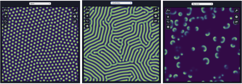
*Figure 1 | Patterns observed via the Gray-Scott model simulation on VisualPDE (“Gray–Scott Model.” VisualPDE, 23 Dec. 2025,* *visualpde.com/nonlinear-physics/gray-scott.html*.)

Each of these patterns emerges from small changes in the model’s parameters, showing how simple variations in the mathematical parameters can produce morphologies which appear visually similar to the diversity observed in nature.

While numerous studies have analyzed reaction-diffusion systems and the emergence of abstract pattern classes such as spots, stripes, and labyrinths¹², there are few educational and exploratory studies that classify these morphologies using species wide/specific comparisons across a broad range of organisms. Many studies focus primarily on the mathematical behavior of the system, rather than on how similar morphologies may visually resemble patterns observed across various biological species. Moreover, factors, such as the organism’s body shape and developmental variations, that may significantly influence real biological development, are either simplified or ignored in simulations¹³. We know that in nature, pattern formation rarely occurs in a perfect environment; rather it is affected by random noise or fluctuations, irregular geometries, and perhaps local factors. Exploring these influences will help us align mathematical models to the actual biological systems.

This study aims to model the natural pattern formation across multiple species using the Gray-Scott framework. It simulates and visually compares the skin surface patterns of six organisms: the cheetah, eel, bacterial colony, poison dart frog, butterfly, and pufferfish. These species were chosen since each of them represent a distinct morphogenetic pattern and highlight the range of complex patterns that can be produced by the mathematical model.

The study classifies simulations by specie-specific morphologies, vs. the shapes of their abstract patterns. Results are judged on a qualitive basis of virtual resemblance to naturally observed patterns. It also introduces different boundary conditions to represent differences in the bodies of species. Stochastic noise is added to examine how randomness or biochemical fluctuations may affect pattern formation across animals.

The study adjusts parameters such as feed (F) and kill rates(k), diffusion ratios, and noise amplitudes. This helps to explore how small mathematical changes can lead to the variety of biological patterns observed across species. The results illustrate the principle of morphogenesis, that the same basic rules, applied under different conditions, can create extraordinary diversity in living organisms.

Methods

Mathematical Model

The Gray-Scott model is a two-species reaction-diffusion system that captures how chemical concentrations evolve over time through reaction and diffusion. It is represented by the following coupled partial differential equations¹⁴:

\frac{\partial U}{\partial t} = D_u \nabla^2 U – UV^2 + F(1-U) \tag 1

\frac{\partial V}{\partial t} = D_v \nabla^2 V + UV^2 – (F+k)V \tag 2

Here, U and V represent two interacting concentration fields within the reaction-diffusion system. In the context of the Gray-Scott framework, U may be interpreted as an activator-like field and V as an inhibitor-like field; however, in this study they are treated as abstract mathematical variables rather than experimentally identified biological morphogens. The diffusion coefficients Du and Dv determine how rapidly each field spreads across space.

The term $D_u \nabla^2 U$ models the diffusion of the activator field $U$ , while $D_v \nabla^2 V$ models diffusion of the inhibitor field $V$ . The nonlinear reaction term $UV^2$ couples the two fields, causing $U$ to be consumed while simultaneously contributing to the production of $V$ . The feed term $F(1-U)$ continuously replenishes the activator field $U$ , while the removal term $-(F+k)V$ causes the inhibitor field $V$ to decay over time. Different combinations of the feed parameter $F$ and kill parameter $k$ generate distinct spatial morphologies such as spots, stripes, labyrinths, and clustered structures. For each pattern, unique values of $F$ and $k$ were chosen to generate morphologies qualitatively resembling patterns observed in nature¹⁵.

Pattern selection

Pattern selection aims to explore and classify the range of spatial morphologies generated by the Gray-Scott reaction-diffusion system. Output patterns were grouped into distinct classes based on their geometric and topological characteristics vs. treating all output structures as a single outcome.

Pattern grouping was guided by two primary criteria:

Morphological distinctness: Each selected pattern class exhibited distinct spatial arrangement, such as isolated spots, connected stripes, hollow rings, or clustered patches. Patterns that differed only in scale or contrast were not considered.
Stability: Only patterns that reached a stable or quasi-stable equilibrium over long simulation times were selected.

Based on the exploratory simulations, four primary pattern classes were identified. These classes were defined according to their geometric characteristics rather than by the identity of the biological specie. The species-inspired simulations presented later in the paper represent specific applications or combinations of these morphology classes.

Hollow spot patterns, characterized by approximately circular voids of low V (inhibitor) values surrounded by high U (concentration) boundaries. The morphology resembles ring-like structures, where pattern contrast is concentrated at the edges vs. the center.
Filled spot patterns, consisting of isolated, approximately circular regions of elevated V inputs embedded within a lower U value background. Unlike hollow spots, these structures are solid rather than ring-shaped¹⁶.
Clustered patch patterns, where concentration accumulates in irregular, cloud-like regions rather than forming discrete, evenly spaced units. These patches often vary in size and shape and may partially merge¹⁷.
Stripe and labyrinth patterns, formed of elongated, connected regions of elevated U values that may curve, split, or form maze-like networks. Some stripes not connected to others may appear as filled spots rather than lines.

Several organism-inspired simulations combined features from multiple patterns. For example, some poison dart frog and eel-inspired morphologies exhibited the spotted and labyrinthine patterns simultaneously. Here, the species-inspired examples were treated as qualitative visual analogies rather than independent mathematical classes.

Numerical Simulation

All simulations were implemented via Python using NumPy for computation and Matplotlib for visualization. The computational domain was kept as a two-dimensional square lattice of size L×L, with L at 200, unless otherwise specified. Periodic conditions were applied at the boundary of the square computational grid through NumPy’s roll() operation, allowing concentration values to wrap continuously across opposite sides of the computational domain. While the outer computational box retained periodic boundary conditions, the mask acted as a constraint, restricting diffusion and reaction dynamics to the inside of the domain.

The initial conditions were kept as U = 1.0 and V = 0.0. Small random perturbations (noise amplitude = 0.05) were added to V at initialization (t = 0) to trigger symmetry breaking and introduce developmental variability into the resulting morphologies. Time evolution was simulated for 1,000-15,000 iterations until the morphology reached a visually stable or quasi-stationary configuration.

Numerical Implementation

The Gray-Scott equations were solved numerically using an explicit finite-difference scheme on the two-dimensional square lattice, as described earlier. Unless otherwise specified, simulations were performed on a grid of size L=200, with a spatial step size Δx=1.0 and time step Δt=1.0. A higher-resolution simulation using L=1000 was additionally conducted for the butterfly-inspired morphology to capture finer structural detail over a longer time.

The diffusion coefficients were fixed throughout the simulations at:

D_u = 0.16, \quad D_v = 0.08

The Laplacian operator $\nabla^2$ was approximated using a standard five-point finite-difference stencil:

\nabla^2 U_{i,j} = U_{i+1,j} + U_{i-1,j} + U_{i,j+1} + U_{i,j-1} – 4U_{i,j}

with an equivalent expression used for the inhibitor field $V$ . Periodic boundary conditions on the outer computational domain were implemented using NumPy’s roll() operation, which wraps neighboring grid values across opposite edges of the lattice.

Initial conditions consisted of broadly homogeneous concentration fields:

U(x,y,0) = 1.0

V(x,y,0) = 0.0

To initiate symmetry breaking, a square perturbation region, centered within the domain, was introduced with the following concentrations:

U = 0.5, \quad V = 0.25

Small, uniformly distributed, random perturbations were added to the inhibitor field $V$ at $t=0$ using NumPy’s pseudo-random number generator.

V(x,y,0) = V(x,y,0) + \sigma \eta(x,y)

where $\eta(x,y)$ is sampled from a uniform distribution on $[0,1)$ and $\sigma$ depicts the noise amplitude. Depending on the simulation, values for $\sigma$ were considered between 0.025 and 0.05. Noise was applied only initially and was kept constant during time evolution.

Pattern evolution was computed iteratively using forward Euler integration. For each iteration, the nonlinear reaction term $uv^2$ was evaluated and used to update both concentration fields in the Gray-Scott equations.

Species-inspired geometric boundaries were implemented using binary masks corresponding to simplified organism shapes such as ellipses, circles, triangular wing structures, elongated domains, and radial protrusion geometries. During each iteration, concentration values outside the mask were set to zero through element-wise multiplication:

U \leftarrow U \cdot M;\quad \quad V \leftarrow V \cdot M

where $M$ is the binary mask defining the active computational domain. This helped restrict the diffusion and reaction dynamics to the interior of the geometry.

Parameter exploration was conducted interactively using slider-controlled simulations by varying $F$ , $k$ and simulation duration across ranges to generate Gray-Scott morphologies. In most cases, parameters were explored at increments of 0.001, especially near transition regions where small parameter changes produced abrupt morphological shifts.

Simulations were run between 1,000 and 15,000 iterations depending on morphology, while the high-resolution butterfly simulation necessitated up to 50,000 iterations to reach a quasi-stationary state. Convergence was assessed by visually examining whether successive iterations produced minimal large-scale structural changes in the resulting morphology.

A pattern was considered stable or quasi-stationary when increasing the number of simulation steps no longer produced significant visual changes in the morphology. Here, stability was assessed by continuing the simulation beyond the emergence of the pattern and observing whether the overall structure, such as the arrangement of spots, stripes, or clusters, remained broadly unchanged. Minor local fluctuations and small-scale variations could still occur, but the dominant morphology and spatial organization remained unchanged.

Different morphologies required different numbers of iterations to stabilize. Simpler clustered or spot-like structures typically formed within a few thousand steps, whereas more complex stripes and labyrinthine patterns required substantially longer simulation times to fully develop and stabilize.

The code can be found here: https://github.com/nagarwal1012/model-for-animal-patterns/tree/main.

Parameter Exploration

To identify biologically realistic patterns, an exploratory parameter scan of F and k values was performed across the following ranges to produce different morphologies:

0.01 \leq F \leq 0.08 \tag3

0.01 \leq k \leq 0.08 \tag4

Final parameter values were selected based on the following conditions:

The pattern consistently emerged from small perturbations of uniform initial conditions.
The morphology remained stable over further time steps.

Boundary and Noise Effects

Additional numerical experiments tested how boundary conditions and random noise levels affected the resulting morphology. Masked and unmasked periodic-domain simulations were compared visually, and the amplitude of initial random noise was varied between 0.01 and 0.1. These variations helped determine the sensitivity of the Gray-Scott system to environmental disturbances.

Results

The Gray-Scott equations produced a variety of morphologies across all simulations, demonstrating how changes in feed-kill parameters, body geometry, noise amplitude, and simulation time can generate visually diverse patterns. Due to the presence of sensitivity to the initial conditions in the reaction-diffusion equations, the resulting patterns vary vastly.

The morphological structures formed as isolated spots, connected stripes/labyrinthine networks, hollow rings, or clustered patches depending on the parameter values¹¹. Stabilization time varied significantly: some patterns emerged within a few thousand iterations, while others required integration over a longer period to fully develop stable features.

A key observation emerged: the Gray-Scott system exhibits strong nonlinearity – visually distinct morphologies often arise from very small changes in the parameters. Rather than varying smoothly, the system moves abruptly between pattern classes, highlighting the existence of multiple stable attractors¹².

Across all experiments, the inhibitor field V(x, y) developed from an initial uniform state into stable structures after several thousand iterations, with each pattern requiring a different number of time steps for stabilization. For the uniformly hollow and filled spots, stripes and labyrinth patterns (which display intricate patterns), the model required between 11,000 and 50,000 steps to achieve convergence to the appropriate structures. In contrast, the irregularly filled and hollow spots, stripes and spots, and clustered patch patterns emerged much faster, requiring only between 2,000 – 5,000 steps. In all cases, the activator-inhibitor concentration was constrained within a boundary, making the influence of shape visible immediately.

One common observation is that the qualitative nature of the pattern depends extremely sensitively on the balance between F and k. This relationship is highly sensitive: even small changes in the parameters can suddenly shift the system into a completely different pattern, such as turning spots into stripes or stripes into more chaotic, wave-like structures¹².

In multiple patterns, particularly the spots, reversing the relative control of F and k (for example, slightly increasing F while decreasing k, or vice versa) caused an inversion. As an example, regions that previously appeared as dark holes surrounded by pigment suddenly got filled, while previously solid areas became hollow. This hole-blob inversion arises because F controls replenishment of activator U, whereas k enhances removal of inhibitor V. On swapping their influence, the system stabilization flips to a “U-dominant” or “V-dominant” configuration. The inversion was especially prominent in the spotted patterns (hollow rings and isolated spots), where the outcomes were complements of each other, depending on the exact (F, k) pairing.

Number

Pattern

1.1

1.2

3.1

3.2

4.1

4.2

6.1

6.2

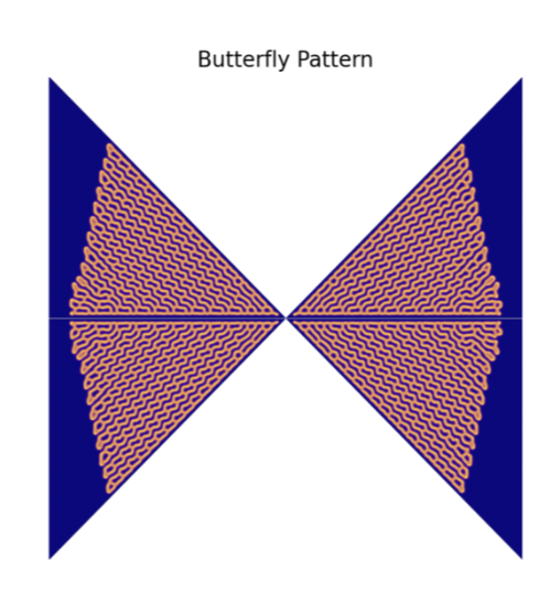
Table 1 | Set of simulated pattern outputs.

Species-inspired example	Major pattern class
Cheetah	Hollow + filled spot patterns
Bacterial colony	Clustered patch patterns
Eel	Hollow + filled spot patterns
Poison dart frog	Stripe and labyrinth patterns + Filled spot patterns
Pufferfish	Stripe and labyrinth patterns
Butterfly	Stripe and labyrinth patterns

Table 2 | Mapped morphologies to pattern classes.

Pattern Formation

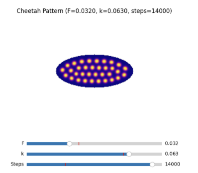
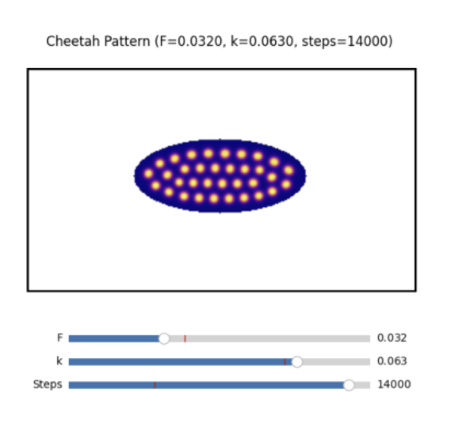
Each simulation produced distinct morphologies that qualitatively resembles patterns observed in nature. Pattern 1.1: Rosettes composed of circular voids surrounded by high contrast boundaries was generated using $F \approx 0.031$ and $0.032$ , $k \approx 0.055$ and $0.063$ respectively. Pattern 1.2 shows different patterns based on different $k$ values: increasing $k$ sharpened the pattern and broke them into smaller, discrete clusters while decreasing $k$ values caused some merger of the patterns. Increasing the noise level in the equations (such as in pattern 3.1 and 3.2) helped us produce irregular rosettes.

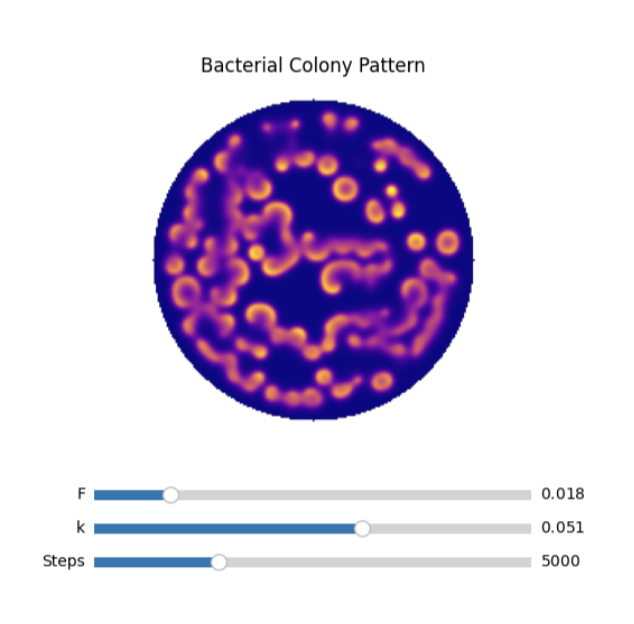
Pattern 2: cloud-like clusters took ~5000 iterations. Here, a low feed rate(F=0.018) and relatively high kill rate (k=0.051) limited the supply of the activator enzyme. This caused the growth to happen primarily at the outermost domain boundary.

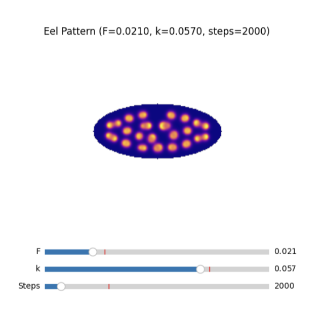
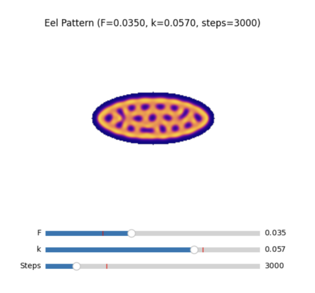
Coming back to pattern 3 (irregularity achieved with noise inclusion), two parameters sets led to patterns 3.1 and 3.2. In 3.1, lower feed (F = 0.021), we get a fine honeycomb or chain-like arrangement of small spots. Increasing F to 0.035 in 3.2 (with k fixed at 0.057) stretched these structures into elongated formations aligned with the long axis. We can see a similarity to the behavior seen in patterns 1.1 and 1.2 in terms of the filling of the gaps and vice versa for different values of F.

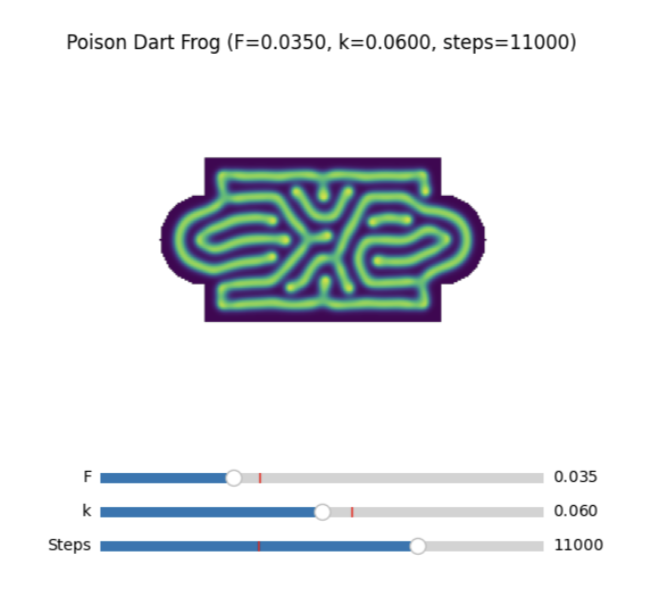
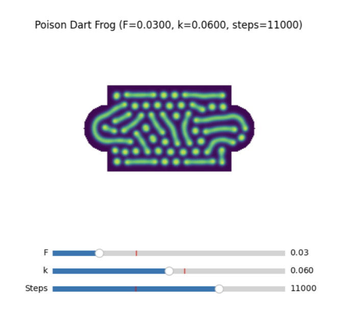
Pattern 4 simulations required more iterations (11,000 steps) to stabilize into distinct spot clusters. The chosen parameters (F = 0.03 and 0.035, k = 0.060) produced different patterns based on F values. Higher F values tended to produce thicker stripes and reduced hollow regions. Small increases in F filled internal voids and thickened the spots, demonstrating the model’s sensitivity to feed-kill balance again.

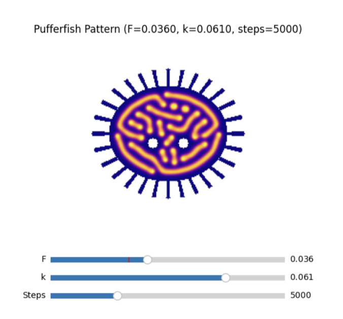
The pattern 5 simulation produced short, closely packed lines distributed almost uniformly across the shape for (F = 0.036, k = 0.061).

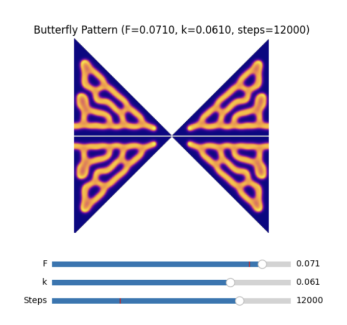
Finally, pattern 6 was generated with two simulations: a standard resolution version (L = 200) and a high-resolution, longer simulation (L = 1000 and 50,000 steps, higher than any other simulation) to capture the fineness of the pattern. The larger domain allowed symmetry-reflected bands and small spot fields to emerge. Parameters with high feed (F = 0.067 and 0.071) and comparatively smaller kill highlighted clustering of the spots.

The study also attempts to move beyond purely qualitative description. It computes three quantitative metrics for each simulation using connected-component analysis on the thresholded inhibitor field V (threshold = mean(V) + 0.4 × range(V); minimum region size 5px²; L = 200, Du = 0.16, Dv = 0.08, σ = 0.05). Metrics are:

number of discrete pattern regions N,
(ii) mean region area Ā (px²), and
(iii) mean nearest-neighbor distance d̄NN between region centroids (px).

Results are summarized in Table 3 below.

Pattern	F	k	Regions (N)	Mean area (px²)	CV area	Mean NN dist (px)
Cheetah (1.1a)	0.031	0.055	1	33791.0	0.00	–
Cheetah (1.1b)	0.032	0.063	164	51.1	0.28	12.4
Bacterial colony (2)	0.018	0.051	105	111.9	0.78	15.1
Eel (3a)	0.021	0.057	186	60.0	0.29	13.1
Eel (3b)	0.035	0.057	1	30673.0	0.00	0.0
Poison dart frog (4a)	0.030	0.060	126	122.2	0.99	13.1
Poison dart frog (4b)	0.035	0.060	46	438.2	1.40	18.9
Pufferfish (5)	0.036	0.061	35	327.8	0.85	14.8
Butterfly (6, L=200)	0.037	0.060	13	1651.4	2.15	41.2

Table 3 | Quantitative morphological metrics across simulations

(L=200, Du=0.16, Dv=0.08, noise=0.05)

The above metrics quantify the visual distinctions described in the above text. Cheetah 1.1a and Eel 3b gave N = 1 because their final morphology is a single connected labyrinthine or filled network rather than discrete spots. The high CV area values for patterns 4b and 6 reflect irregular, mixed-size structures, consistent with the visual description of these patterns as spot-stripe hybrids or bilaterally symmetric bands. The large mean d̄NN distance for the butterfly simulation (41.2px) reflects its coarser stripe spacing relative to the spot-dominated patterns (12–19 px). These values are reported for a single representative simulation per parameter set. Replicating these statistics further and examining sensitivity to threshold choice form scope for future work.

Parameter Sensitivity

The morphology of the resulting pattern is governed primarily by the balance between replenishment of U through F and removal of V through k. Increasing F while keeping k constant thickens stripes, fills hollow regions, and increases clustering. Increasing k while keeping F constant sharpens boundaries, breaks continuous structures, and suppresses large-scale growth. This leads to the hole-blob inversion where hollow spots transform into filled spots or vice versa under slight parameter shifts.

Parameter sensitivity increased with simulation duration. Patterns that appeared similar at 2,000 steps diverged significantly after 10,000-15,000 iterations. This was especially evident in high-resolution simulations (L = 1000), where minor parameter adjustments led to entirely different symmetries.

To more systematically document the parameter exploration, a low-resolution F–k phase diagram was generated by running simulations across a 25×25 grid of parameter values (F ∈ [0.010, 0.075], k ∈ [0.040, 0.075]) on an L = 80 grid for 4,000 iterations each. Each cell was classified into one of five morphological regimes: uniform, spots, stripes/mixed, labyrinths, or filled/dense using connected-component analysis on the thresholded V field.

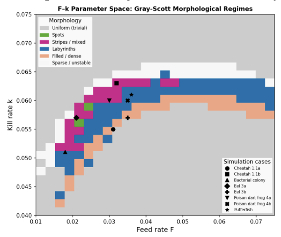
Figure 2 shows that the six organism-inspired parameter sets occupy a distinct region of the diagram. Specifically, cheetah simulations (1.1a, 1.1b), eel (3a, 3b), bacterial colony, poison dart frog (4a, 4b), and pufferfish lie at boundaries between regime regions. This is consistent with the observation of high sensitivity: abrupt morphological transitions for small parameter changes. The butterfly simulation (F ≈ 0.037, k ≈ 0.060) sits within the labyrinths/stripes region. Three replicate runs (distinct random seeds 42, 99, 137) were performed for the cheetah (1.1b) and poison dart frog (4a) sets. In all replications the same morphological class was generated, confirming robustness of the classification to randomness or noise factor. Note that parameter selection in this study was performed by visual assessment of morphological similarity to biological patterns.

Discussion

The results clearly demonstrate that the Gray-Scott reaction-diffusion framework can generate a wide range of spatial morphologies depending on the parameters, noise, and boundary conditions. While the results section focused on characterizing these patterns mathematically, an important observation is noticed when these morphologies are observed together. Many of the simulated patterns show a visual resemblance to pigmentation patterns observed in real biological organisms. This section discusses these similarities, examines the role of geometry and noise in shaping them, evaluates their plausibility, outlines the limitations of the model and its possible extensions.

Similarity to Animal Species

Although the Gray-Scott equations are abstract and do not model biological identity, in this study, the variables U and V are treated as abstract mathematical concentration fields rather than experimentally identified enzymes or biological morphogens¹⁸. Importantly, the visual similarities were not imposed by the model; rather, they emerged from the mathematical framework applied under different conditions.

Pattern 1 (the rosette-like pattern with hollow and filled spots) is qualitatively similar to the coat patterns of large felids such as cheetahs¹⁹. Hollow rings and solid spots both occur together when the parameter values are closely related – qualitatively comparable to the variation that can be seen both within and among different felid species. In the simulations, minor changes in F and k caused fragmentation, merging, or inversion of these structures, which suggests that small changes within a reaction-diffusion framework could produce visually similar patterns. Pattern 2 (the clustered patch pattern) showed dense, irregular concentrations near the boundaries in circular domains, mirroring the way bacterial colonies grow. Since the appearance of any particular bacterial colony depends on how the sample is positioned in the petri dish and the same colony can appear in two very different ways when viewed from different positions, it was not possible to compare it with any specific colony; instead, pattern 2 was judged to visually resemble bacterial colonies. Pattern 3 (the irregular spots and holes) showed directional alignment along the long axis of the boundary in narrow or elongated domains. This behavior qualitatively matches the longitudinal striping found in organisms such as eels, in which the shape of the body strongly influences the orientation of the pattern. Notably, this alignment appeared without having directionality explicitly programmed into the equations, showing that the geometry is sufficient to bias the development of the pattern. Pattern 4 (the high-contrast combination of spots and stripes) is like the striking pigmentation of poison dart frogs. These patterns had irregular spacing and vary in size, especially in the presence of noise: this is comparable to the variation between real life organisms. Pattern 5 (the combination of spots and stripes) adapted to both the central body and the extended parts, resembling the surface patterns of a pufferfish. The fact that the patterns continued across curved and projecting areas demonstrates that reaction-diffusion systems can adapt to complex geometric constraints. Finally, pattern 6 (the symmetric pattern) is like the wing patterns of butterflies, in which mirror-image structures naturally occur across the body axis within domains that are bilaterally constrained. For these simulations, symmetry was not imposed algorithmically but emerged because of the interaction between the boundary geometry and the reaction-diffusion dynamics.

Importantly, these simulations do not claim to reproduce exact biological pigmentation mechanisms. Instead, they demonstrate that the visual essence of animal patterns can be modelled using the same mathematical principles under different conditions.

Role of Boundary Conditions on Pattern Formation

A key difference of this model from many classical reaction-diffusion studies is the use of finite, species-inspired boundaries. Rather than assuming infinite or perfectly periodic domains, each simulation constrained pattern formation within a simplified geometric representation of an organism’s body.

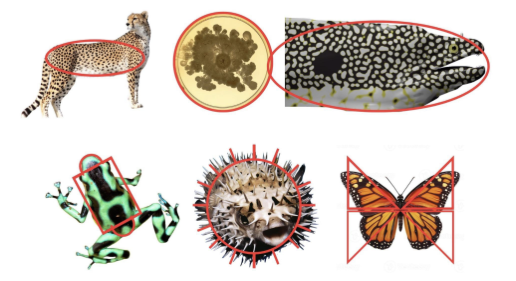
*Figure 3 | Boundary geometry inspired by animal shapes*.

The geometry of the organism’s boundary influenced the resulting patterns. Because concentration values outside the mask were forced to zero at every iteration, pattern formation near mask edges was suppressed; locally constraining the patterns. These geometric influences suggest that boundary geometry may play an important role in shaping reaction-diffusion morphologies. Near edges, diffusion was limited, suppressing pattern formation or distorting spot and stripe structures. In elongated domains, stripes preferentially aligned with the longest dimension, while in circular or oval domains, spots arranged radially²⁰. In more complex geometries, such as the pufferfish boundary with radiating extensions, patterns adapted to the shape locally: bending, fragmenting, or terminating near protrusions. To isolate the effect of geometry, an explicit comparison experiment was conducted using identical parameters (same grid size, F, k, noise amplitude, and number of iterations) with and without boundary constraints. This allowed the role of the boundary to be assessed, independent of the reaction-diffusion dynamics.

With boundary

Without boundary

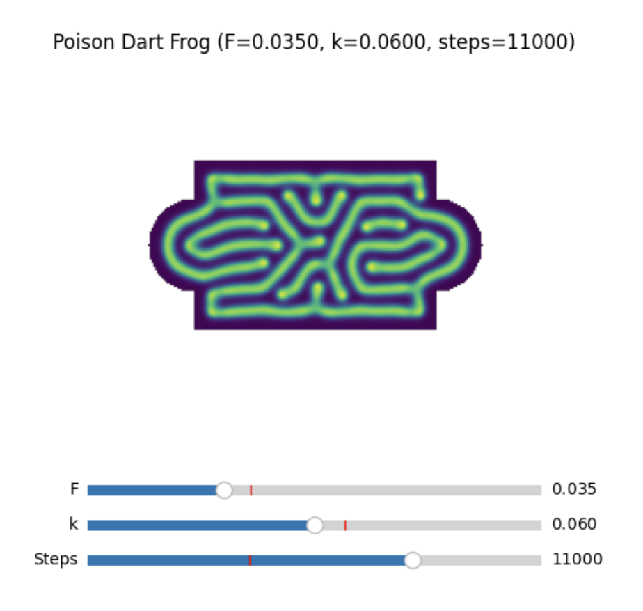
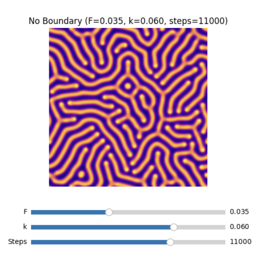
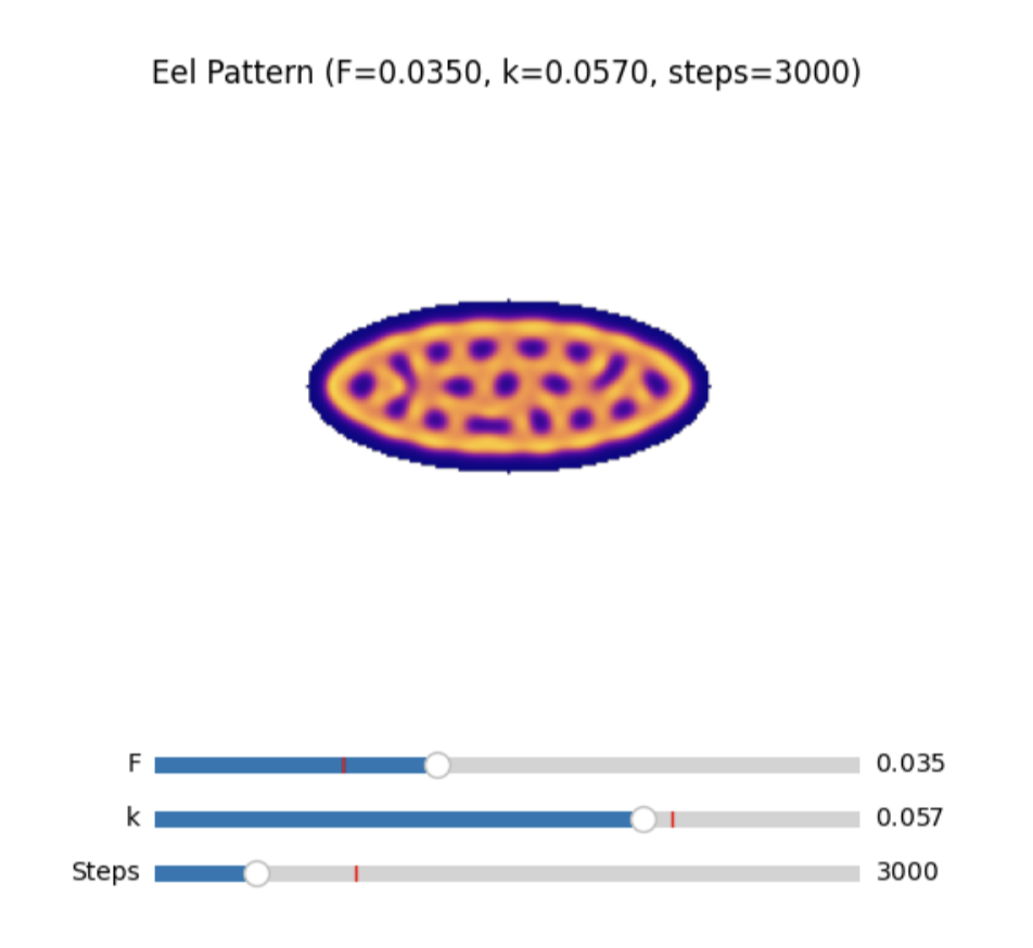
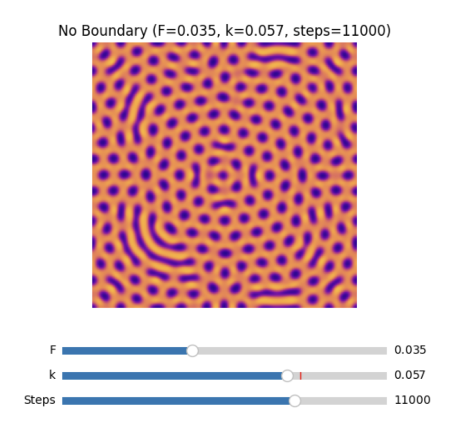
Table 4 | Effect of boundary conditions on resulting patterns.

In the poison dart frog simulation, the boundary condition system produced irregular, high-contrast stripe-spot hybrids within the body boundaries. Pattern terminated near the edges, and stripe segments curved and adapted to the geometry. In contrast, when the same parameters were applied without any boundary, the system evolved into a nearly uniform labyrinthine pattern that tiled the entire domain evenly. The animal-like localization and spatial variation disappeared entirely, despite unchanged underlying equations and parameters. A similar effect was observed in the eel simulation. With an elongated boundary, the pattern aligned along the major axis of the domain, producing spotted structures oriented lengthwise. Without the boundary, the same parameters generated a uniform pattern, consisting of regularly spaced spots with no preferred direction. The loss of alignment demonstrates the impact of the diffusion constraints imposed by the boundary.

Influence of Noise

Stochastic noise played a crucial role in transforming the mathematically derived patterns into biologically plausible ones. Additive random noise was introduced in the simulations at the initial stage. This represents naturally occurring biochemical fluctuations during early development and developmental variability in organisms. In the numerical implementation, noise was added directly to the inhibitor concentration field V(x,y) at initial stage:

V(x,y,0) = V_0(x,y) + \sigma \eta(x,y) \tag5

where $\eta(x,y)$ is a spatially uncorrelated random field sampled from a uniform distribution on $[0,1)$ , and $\sigma$ denotes the noise amplitude. In all final simulations, $\sigma = 0.05$ .

The modified model of the form thus can be represented as:

\frac{\partial U}{\partial t} = D_u \nabla^2 U – UV^2 + F(1-U) \tag6

\frac{\partial V}{\partial t} = D_v \nabla^2 V + UV^2 – (F+k)V + \sigma \eta(x,y) \tag7

with the stochastic term acting as an initial perturbation rather than a continuously injected noise source. This choice aims to replicate biological development, where random fluctuations influence early morphogenesis vs. acting uniformly throughout the life of the organism.

Equations (6) and (7) above are written in the form of continuous stochastic partial differential equations (PDEs) only as a compact mathematical shorthand. In the actual numerical implementation, the noise term $\eta(x, y)$ was applied at $t = 0$ , as a one-time additive perturbation to $V$ before the time-stepping. No noise was injected for any subsequent iteration. Equations (6) and (7) therefore represent the modified initial state, not a continuous system. To remove any ambiguity, the stochastic notation in these equations could be expressed as a modified initial condition:

V(x, y, 0) \leftarrow V(x, y, 0) + \sigma \eta(x,y),

with the PDEs (6) and (7) then becoming the standard deterministic Gray-Scott equations for $t > 0$ .

Noise amplitude was observed to play a central role. The noise level used in the final experiments (0.05 for all trials) produced realistic irregularities. The slight asymmetries, spot-size variability and pattern defects qualitatively resemble the deviations between members of the same species. For lower noise values, the model produced highly regular, almost symmetric, and repetitive patterns. While this is mathematically stable, such results lack the imperfections that commonly occur in real biological organisms. On the other hand, higher noise levels disrupted the symmetry, introduced variations in spot size and spacing, and generated some local defects, producing real-life like variations observed between individuals of the same species. This can be observed in the eel and cheetah patterns.

To isolate the effect of noise amplitude, an additional controlled experiment was conducted using identical parameters (same domain size, $f$ , $k$ , boundary conditions, and number of iterations) while changing only the noise. Specifically, patterns were compared for $\sigma = 0.05$ and $\sigma = 0.025$ in both the bacterial colony and butterfly simulations.

Noise = 0.05

Noise = 0.025

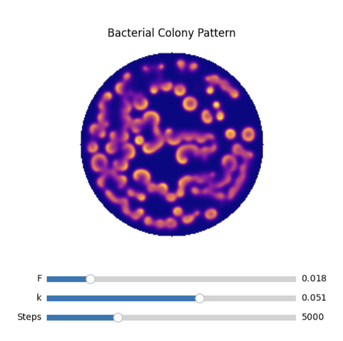
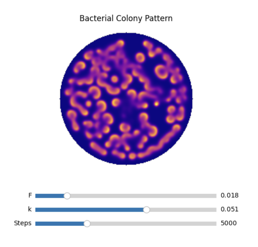
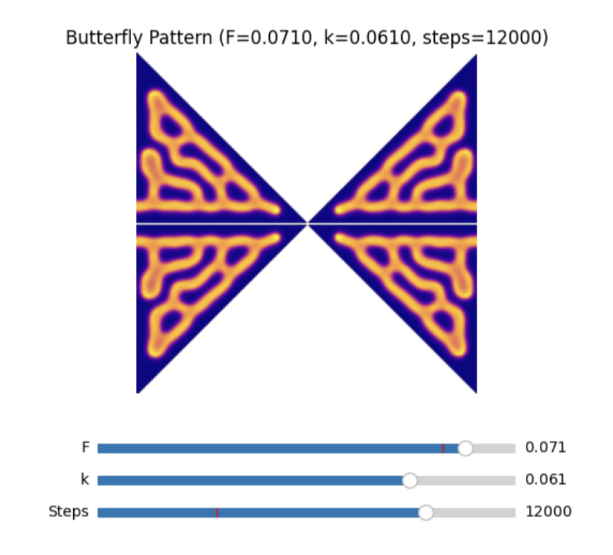
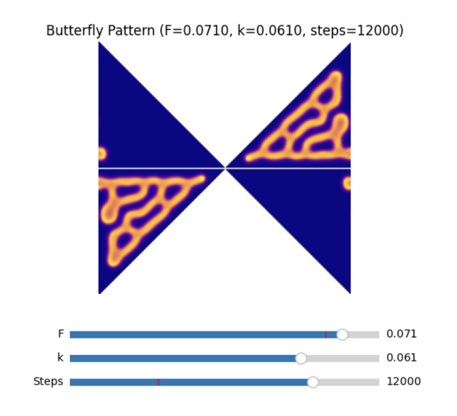
Table 5 | Effect of changes in noise on resulting patterns.

Reducing the noise amplitude from σ = 0.05 to σ = 0.025 produced smoother, more regular patterns with fewer local defects in both the bacterial colony and butterfly simulations. While the overall morphology class was unchanged, higher noise generated greater asymmetry and variability, producing patterns that better resemble the biological reality. In contrast, lower noise factor resulted in cleaner but visually less natural-looking wing patterns.

Across the two noise values, lower noise led to significantly reduced fine-scale variability without altering the fundamental pattern class. Conversely, higher noise levels led to destabilization and partial loss of coherence in the structure. The chosen noise amplitude of 0.05 therefore represented a balance between order and disorder.

In summary, lower noise values resulted in highly uniform patterns, while higher values destabilized the system, leading to fragmentation or chaos. Importantly, noise did not change the fundamental pattern but modified the structure, suggesting that stochasticity contributes primarily to variations within the pattern vs. its main identity. This is qualitatively consistent with biological observations, where unexplained or random factors cause developmental variations without completely disrupting overall pattern structure.

Parameter Sensitivity and Biological Plausibility

Although the Gray-Scott system shows strong sensitivity to parameter variation, real biological organisms are understood to possess additional bio-regulatory mechanisms that reduce excessive variations. Thus, while reaction-diffusion dynamics may contribute to the diversity of natural pigmentation patterns, biological systems must also balance this sensitivity with mechanisms that ensure the formation of reliable and repeatable patterns.

Overall, these findings show how reaction-diffusion systems subjected to different feed-kill balances, noise conditions, and boundary geometries can generate a wide range of morphologies qualitatively and visually resembling biological patterns. The results are consistent with the original theoretical ideas proposed by Alan Turing that complex biological forms may arise from simple chemical rules (modeled here mathematically). At the same time, they also highlight the practical importance of boundary conditions and stochasticity, two factors that substantially influence the resulting morphologies within this exploratory mathematical framework.

Limitations of the Model

The model is yet unable to correlate or map the model variables to real life factors. For instance, the variables U and V do not correspond to specific biological morphogens. Instead, they function as abstract mathematical variables for exploring general reaction-diffusion behavior²¹. First, real pigmentation involves complex gene regulatory networks, cell differentiation, and tissue interactions²² that are not explicitly represented²³ in this model. Second, the geometry of each organism was static throughout the simulation. Body shapes grow and deform over time and interacting dynamically with pattern formation. Finally, the simulations were restricted to two-dimensional domains. Most biological patterns develop in 3D, on curved or three-dimensional surfaces, which can significantly affect diffusion dynamics²⁴. These limitations suggest that the model should be interpreted as a conceptual and theoretical tool, rather than a biological simulator.

Conclusion

The results of this research reveal that the reaction-diffusion model introduced by Gray and Scott is capable of producing many morphologies which resemble various biological patterns. The findings from this research indicate that the variation in parameters, boundaries and noise can lead to different forms of morphologies created with the use of this model one of the most important results obtained in this study is the high sensitivity of the morphologies to slight changes in the parameters of feed and kill rates. The change in these parameters even with a change as small as 0.001 can lead to a complete switch to a fully different morphology. This indicates the non-linear process of behavior of the model and multiple attractors in the phase space of parameters. Boundaries inspired by finite species were necessary to create morphologies more similar to the animal’s actual shape. The comparison of morphologies generated with and without boundaries indicates that the geometry of form influences their behavior concerned with direction and symmetry. Noise was used to create a variation in idealized patterns. It was found out that moderately strong noise produced the best results in terms of biological plausibility of the forms while weak noise led to their regularity.

References

I. Salazar-Ciudad, J. Jernvall. A computational model of teeth and the developmental origins of morphological variation. Development Genes and Evolution. Vol. 212, pg. 1–15, 2011, https://doi.org/10.1007/s00427-011-0378-0. [↩]
B. L. M. Hogan. Morphogenesis. Cell. Vol. 96, pg. 225–233, 1999, https://doi.org/10.1016/S0092-8674(00)80562-0. [↩]
A. Gierer, H. Meinhardt. A theory of biological pattern formation. Kybernetik. Vol. 12, pg. 30–39, 1972, https://doi.org/10.1007/BF00289234. [↩]
A. M. Turing. The chemical basis of morphogenesis. Philosophical Transactions of the Royal Society of London Series B: Biological Sciences. Vol. 237, pg. 37–72, 1952, https://doi.org/10.1098/rstb.1952.0012. [↩] [↩]
Q. Ouyang, H. L. Swinney. Transition from a uniform state to hexagonal and striped Turing patterns. Nature. Vol. 352, pg. 610–612, 1991, https://doi.org/10.1038/352610a0. [↩]
J. D. Murray. Mathematical biology II: Spatial models and biomedical applications. Interdisciplinary Applied Mathematics, Vol. 18. Springer, 2003. [↩]
E. J. Crampin, P. K. Maini. Reaction-diffusion models for biological pattern formation. Methods and Applications of Analysis. Vol. 8, pg. 415–428, 2001. [↩]
A. D. Economou, A. Ohazama, T. Porntaveetus, P. T. Sharpe, S. Kondo, M. Basson, A. Gritli-Linde, M. Cobourne, J. B. Green. Periodic stripe formation by a Turing mechanism operating at growth zones in the mammalian palate. Nature Genetics. Vol. 44, pg. 348–351, 2012, https://doi.org/10.1038/ng.1090. [↩]
S. Kondo, R. Asai. A reaction-diffusion wave on the skin of the marine angelfish Pomacanthus. Nature. Vol. 376, pg. 765–768, 1995, https://doi.org/10.1038/376765a0. [↩]
J. Raspopovic, L. Marcon, L. Russo, J. Sharpe. Digit patterning is controlled by a Bmp-Sox9-Wnt Turing network modulated by morphogen gradients. Science. Vol. 345, pg. 566–570, 2014, https://doi.org/10.1126/science.1252960. [↩]
J. E. Pearson. Complex patterns in a simple system. Science. Vol. 261, pg. 189–192, 1993, https://doi.org/10.1126/science.261.5118.189. [↩] [↩]
A. Tok-Onarcan, N. Adar, I. Dag. Wave simulations of Gray-Scott reaction-diffusion system. Mathematical Methods in the Applied Sciences. Vol. 42, pg. 5566–5581, 2019, https://doi.org/10.1002/mma.5534. [↩] [↩] [↩] [↩]
I. Ali, M. T. Saleem. Spatiotemporal dynamics of reaction-diffusion system and its application to Turing pattern formation in a Gray-Scott model. Mathematics. Vol. 11, pg. 1459, 2023, https://doi.org/10.3390/math11061459. [↩]
A. Adamatzky. Generative complexity of Gray-Scott model. Communications in Nonlinear Science and Numerical Simulation. Vol. 56, pg. 457–466, 2017, https://doi.org/10.1016/j.cnsns.2017.08.021. [↩]
S. Kondo, T. Miura. Reaction-diffusion model as a framework for understanding biological pattern formation. Journal of Physics: Conference Series. Vol. 1531, pg. 012058, 2020, https://doi.org/10.1088/1742-6596/1531/1/012058. [↩]
T. Kolokolnikov, M. J. Ward, J. Wei. On ring-like solutions for the Gray-Scott model: Existence, instability and self-replicating rings. European Journal of Applied Mathematics. Vol. 16, pg. 201–237, 2005, https://doi.org/10.1017/S0956792504006226. [↩]
H. Meinhardt. Pattern formation in biological development. Progress in Biophysics and Molecular Biology. Vol. 59, pg. 1–32, 1993, https://doi.org/10.1016/S0079-6107(05)80001-6. [↩]
M. Watanabe, S. Kondo. Is pigment patterning in fish skin determined by the Turing mechanism? Trends in Genetics. Vol. 31, pg. 88–96, 2015, https://doi.org/10.1016/j.tig.2014.11.005. [↩]
R.-T. Liu, S.-S. Liaw, P. K. Maini. Two-stage Turing model for generating pigment patterns on the leopard and the jaguar. Physical Review E. Vol. 74, pg. 011914, 2006, https://doi.org/10.1103/PhysRevE.74.011914. [↩]
H. Shoji, Y. Iwasa, S. Kondo. Directionality of stripes formed by anisotropic reaction-diffusion models. Journal of Theoretical Biology. Vol. 214, pg. 549–561, 2002, https://doi.org/10.1006/jtbi.2001.2480. [↩]
S. Chen, J. Shi, G. Z. Chen. Spatial pattern formation in activator-inhibitor models with nonlocal dispersal. Discrete and Continuous Dynamical Systems-Series B. Vol. 26, pg. 2157–2185, 2021. [↩]
K. J. Painter, P. K. Maini, H. G. Othmer. Stripe formation in juvenile Pomacanthus explained by a generalized Turing mechanism with chemotaxis. Proceedings of the National Academy of Sciences. Vol. 96, pg. 5549–5554, 1999, https://doi.org/10.1073/pnas.96.10.5549. [↩]
A. Nakamasu, G. Takahashi, A. Kanbe, S. Kondo. Interactions between zebrafish pigment cells responsible for the generation of Turing patterns. Proceedings of the National Academy of Sciences. Vol. 106, pg. 8429–8434, 2009, https://doi.org/10.1073/pnas.0808622106. [↩]
Z. Han, H. Wang, J. Wang, J. Wang. A simple method of shape transformation using the modified Gray-Scott model. Extreme Mechanics Letters. Vol. 69, pg. 102167, 2024, https://doi.org/10.1016/j.eml.2024.102167. [↩]